Estimating causal effects of time-dependent exposures on a binary endpoint in a high-dimensional setting

(1)

R E S E A R C H A R T I C L E

Open Access

Estimating causal effects of

time-dependent exposures on a binary

endpoint in a high-dimensional setting

Vahé Asvatourian

1,2*

, Clélia Coutzac

3,4

, Nathalie Chaput

3,5

, Caroline Robert

4,6

, Stefan Michiels

1,2

and Emilie Lanoy

1,2

Abstract

Background:Recently, the intervention calculus when the DAG is absent (IDA) method was developed to estimate

lower bounds of causal effects from observational high-dimensional data. Originally it was introduced to assess the effect of baseline biomarkers which do not vary over time. However, in many clinical settings, measurements of biomarkers are repeated at fixed time points during treatment and, therefore, this method needs to be extended. The purpose of this paper is to extend the first step of the IDA, the Peter Clarks (PC)-algorithm, to a time-dependent exposure in the context of a binary outcome.

Methods:We generalised the so-called“PC-algorithm”to take into account the chronological order of repeated measurements of the exposure and proposed to apply the IDA with our new version, the chronologically ordered PC-algorithm (COPC-algorithm). The extension includes Firth’s correction. A simulation study has been performed before applying the method for estimating causal effects of time-dependent immunological biomarkers on toxicity, death and progression in patients with metastatic melanoma.

Results:The simulation study showed that the completed partially directed acyclic graphs (CPDAGs) obtained using COPC-algorithm were structurally closer to the true CPDAG than CPDAGs obtained using PC-algorithm. Also, causal effects were more accurate when they were estimated based on CPDAGs obtained using COPC-algorithm. Moreover, CPDAGs obtained by COPC-algorithm allowed removing non-chronological arrows with a variable measured at a time tpointing to a variable measured at a time t´ wheret´<t. Bidirected edges were less present in CPDAGs obtained with the COPC-algorithm, supporting the fact that there was less variability in causal effects estimated from these CPDAGs. In the example, a threshold of the per-comparison error rate of 0.5% led to the selection of an interpretable set of biomarkers.

Conclusions:The COPC-algorithm provided CPDAGs that keep the chronological structure present in the data and thus allowed to estimate lower bounds of the causal effect of time-dependent immunological biomarkers on early toxicity, premature death and progression.

Keywords:Repeated measures, Immunotherapy, PC-algorithm, IDA, High dimensional setting, Causal inference, Observational data

* Correspondence:[email protected]

Part of this work has been presented at the 37thInternational Society Clinical Biostatistics conference in Birmingham, 21st_-25th_{August 2016}

1_{Université Paris-Saclay, Univ. Paris-Sud, UVSQ, CESP, INSERM, Villejuif, France} 2_{Service de Biostatistique et d}_’_{Epidémiologie, Gustave-Roussy, Villejuif, France} Full list of author information is available at the end of the article

(2)

Background

The Intervention calculus when the directed acyclic graph (DAG) is absent (IDA) method was recently developed to estimate lower bound of total causal effects

from observational data in high-dimensional settings [1].

It was originally introduced to evaluate the effect of time-fixed exposure (gene expression). This method is a combination of Peter Clarks (PC)-algorithm [2] and Pearl’s

do calculus [3]. The PC-algorithm is a constraint-based

method for causal structure learning, meaning that it learns the causal structure based on the conditional dependencies of the observational distribution. The out-put of the PC-algorithm results in a CPDAG (completed partially DAG) that encodes conditional dependencies of the data in a class of DAGs (Directed acyclic graphs)

called Markov Equivalent. Then, based on the DAGs in

theMarkov Equivalence Class, causal effects are estimated using Pearl’s do calculus (see section Causal effect estima-tion in high dimensional settings). However, in many clin-ical settings, time-dependent biomarker values under treatment or changes in biomarkers from baseline are of interest. If the true DAG was known, the commonly used marginal structural model (MSM) approach could be used to estimate causal effects in the case of time-dependent

covariates and outcome [4, 5]. In our setting, the true

DAG being unknown, causal effects could not be identi-fied using MSM.

In the 2010s, new anti-cancer treatments targeting mune checkpoints were introduced: the wave of these im-munotherapies began with the anti CTLA-4 treatment which showed a survival benefit in patients with

meta-static melanoma [6, 7]. More recently, promising results

in lung and kidney cancers have also been obtained [8].

Nevertheless, only a subgroup of patients seem to benefit from this treatment: about 20% of patients with metastatic melanoma treated with ipilimumab were long-term

survi-vors (3 years) [9]. Moreover, immune-related toxicity such

as colitis occurs in 8 to 22% of treated patients [10]. The

goal of immunotherapy is to amplify the immune system response against cancer cells. Thus, one can observe the evolution of the treatment by looking at the immune system. Predictive and/or prognostic markers are ideally validated through clinical trials including randomized studies, which are the gold standard [11,12]. Before being evaluated in randomized trial, candidate immunological biomarkers can be identified from high-dimensional data, collected in an observational or non-randomized setting.

Our objective was to develop methods to identify the causal effects of time-dependent exposures on a binary endpoint in a high-dimensional setting, with an application

of time-dependent immunological biomarkers in a

non-randomized prospective study in oncology. However, the PC-algorithm has never been applied on data measured repeatedly at a fixed time points, and the chronological

order among data is not respected when using

PC-algorithm. The first step was then to find the true CPDAG by extending the PC-algorithm to chronologically ordered measures and then to estimate robust causal effects based on the CPDAG estimated using our version of the PC-algorithm. To ensure the accuracy and the efficiency of our method, we made a simulation study where we

com-pared the CPDAGs’structure obtained using PC-algorithm

and our method. Then we compared the estimation of true causal effects calculated based on CPDAGs obtained from both methods. Due to collinearity among time-dependent

biomarkers, we added for the first time the Firth’s

correc-tion while estimating causal effects to avoid instability of the maximum likelihood estimates. After the simulation study, we applied both PC-algorithm and our method to real dataset of time-dependent immunological biomarkers.

Methods

Graph definitions and notations

LetG(N,E) be a graph consisting of nodesNand edgesE.

Nodes represent random variables N= {X1,…,Xp} and

edges represent the links between them. An edge can be either directed Xi→Xj (in this case, Xi is a parent of Xj

and Xj is a descendant of Xi) or undirected Xi−Xj. A

graph with only undirected edges is said to be an undir-ected graph whereas a dirundir-ected graph is made of only directed edges. A partially directed graph contains both directed and undirected edges.

Two nodes are said to be adjacent if they are connected by an edge (either directed or undirected). A path is a sequence of nodes in which all pairs are adjacent. A path

can be eitheropenorclosed. A path is open when there is

no collision between two arrows pointing to the same

node on the path (i.e. the path from Xi to Xm in (1) is

open).

Xi→Xj→Xk→Xm←Xl ð1Þ

A path is closed when there is a collision between two arrows which point to the same node of the path, this variable is a collider (i.e, the path from Xi toXlin (1) is

closed). We denote Xk as a descendent ofXi(and Xian

ancestor ofXk) if there is a path that starts fromXiand

ends to Xk by following the direction of the arrows (1).

We also denote pa(Xi,G) as the parents of Xi in G by

the set of variables pointing to Xi. A graph is called

(3)

complete DAG is non-informative because a lack of arrow means an absence of a direct causal effect.

A graph encodes (conditional) independence

relation-ships through the concept of d-separation [13]. If two

nodes are d-separated by a set of nodes, then the variables corresponding to the nodes are conditionally independent given this set of variables. The set of these given variables

is then called separation set S. Multiple DAGs can be

compatible with a same set of underlying conditional independences. Let a skeleton be the graph obtained by

removing all arrowheads from the DAG and the

v-struc-turesa subgraph of 3 nodes filling two conditions: 1) both arrows are not pointed on Xj(Xjis not a collider) and 2)

whereXiandXkare not adjacent.

The DAGs Xi→Xj→Xk, Xi←Xj←Xk and Xi←Xj→

Xk in which the two conditions hold, belong to the same

Markov equivalence class and are called Markov

equiva-lent. A whole equivalence class can be summarised in a

graph that has the same skeleton and includes the directed arrows of all DAGs in the equivalence class. Edges which are directed differently across the DAGs in the equiva-lence class are represented with bidirected arrows (or sim-ply edges). This graph with both undirected and directed

edges is called aCompleted Partially DAG(CPDAG).

Causal effect estimation in high dimensional settings

IDA

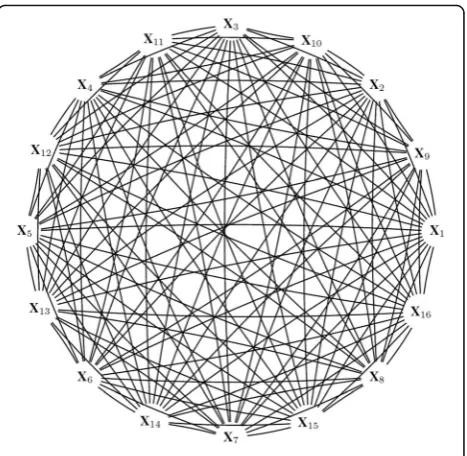
When the relationships between variables are not oriented, the DAG cannot be identified. With many variables in a high-dimensional setting, it is not possible to determine which nodes are ancestors and which are descendants. The only possible initial graph that can be drawn based on high-dimensional data is a complete undirected graph

which is non-informative (Fig.1). The intervention calculus

when the DAG is absent (IDA) method has been intro-duced to determine the CPDAG from the observational data and to estimate lower bounds of the absolute values of the total causal effects in the case where all variables

(including outcome) are continuous [1]; and has been

extended to the case where all variables are binary [14].

The first objective of the IDA is to estimate the CPDAG and its Markov equivalence class that contain the true causal DAG from the observational data by using a causal

learning algorithm such as the PC-algorithm [2]. Then the

intervention calculus [3,15] is used on themDAGsjof the

Markov equivalence classj= 1,…,m, to estimate thep×m

matrixΘof causal effectsθijof each covariateXi(i= 1,…, p) onY.

However, estimating the true causal effect is impossible when a unique DAG is not identifiable. To determine whether or not a covariate has a potential causal effect, the minimum absolute causal effect of a covariate is defined ascβ_i¼ minjðj^θijjÞ. Then a ranking of covariates’

causal effects is made based on these lower bounds, where ^

βi1is the lower bound of the covariateiwith the rank 1:

^

βi1≥β^i2≥…≥^βip: ð2Þ

Determining all the DAGs that are present in the Markov equivalence class can be highly computationally intensive in a high-dimensional setting. Nevertheless, rather than computing all the DAGs, it is still possible to determine the set of parents used for adjusting by extracting them from the CPDAG. The local algorithm

used by Maathuis et al. [1] checks if the parents are

locally valid (if they create or not a new collider) in the

CPDAG and all causal estimates for a single covariateXi

on Y are in the multiset Θi= {θij}j∈{1,…,m} and i∈{1,…,p}. Contrary to a set, in a multiset the replication of an element matters. For instance, the multisets {a,a,b} and {a,b} are not equal while the sets {a,a,b} and {a,b} are. The multiset allows the multiplicity of an element.

Finally, the assumptions made in the IDA are: (A1) There are no hidden variables.

(A2) The joint distribution of covariates Xi, …, Xp is

normal and faithful to the true (unknown) DAG. (A3) CovariatesXi,…,Xphave equal variance.

The IDA method developed by Maathuis et al. is

implemented in the R-package pcalg [16].

PC-algorithm

The PC-algorithm is a constraint based method for causal structure learning [2,17], meaning that it learns the causal structure based on the conditional dependencies between

(4)

variables. A sketch of the PC-algorithm is given in algorithm 1.

First, it estimates the skeleton of the underlying structure by checking all given conditional dependencies between each variable at a significance levelα. If no information on dependencies is given, then the graph used as input is an

undirected graphsuch as in Fig.1. Once the skeleton is

ob-tained, edges are oriented in the v-structures to meet the

conditional dependencies and finally the CPDAG is ob-tained by directing as many remaining edges as possible ac-cording to three rules (see section 3.1 of [18]):

R1: When there is a directed edge Xi→Xj, Xj−Xk is

oriented intoXj→XkwithXiandXknot adjacent;

R2: When there is a chain Xi→Xk→Xj, Xi−Xj is

oriented intoXi→Xj;

R3: When there are two chains Xi−Xl→Xj and Xi−

Xk→Xj, Xi−Xj is oriented into Xi→Xj with Xk and

Xlnot adjacent.

Even though the PC-algorithm has been shown to be

consistent in high-dimensional settings [19], one of its

issues remains the effect of the set of ordered variables

Oin the final output. In fact, the order of the variables

determines which pair of nodes is tested first, determining which edges are removed first and so affecting which tests are considered later on. This order dependence impacts robustness of the results in high-dimensional settings. Two different solutions have been suggested: the stability ranking and the PC-stable, which will be outlined below. Before running the algorithm, the multiple testing requires to specify the

significance level (cut-off ) α for the conditional

independence tests. In fact, settingα to a certain value

means that only conditional dependencies with a

p-value under α are kept. Thus, running PC-algorithm

with a small value of alpha leads to obtaining sparser graphs.

Stability selection

To deal with the order dependence issue of the PC-algorithm in the IDA which can lead to poor robust-ness, Stekhoven et al. proposed to add a stability

selec-tion step [20] to IDA. This method, called Causal

Stability Ranking (CStaR) [21], is based on a re-sampling

approach. The IDA is run over 100 independent random subsamples and then in each subsampling run, the

vari-ables are ranked according to Eq. (2). At the end of all

runs, the relative frequencies Πi of covariates appearing

among the top of qvariables are used to define a stable

ranking:

^

Π1≥Π^2≥…≥Πp^ : ð3Þ

For a givenq, a bound for the per-comparison error rate

(PCER), which can be seen as the false positive error rate, is given by:

1 2Πjc−1

q2

p2: ð4Þ

PC-stable

Another approach that considers the order dependence issue of the PC-algorithm was explored by Colombo and Maathuis by introducing an order-independent

version of the PC-algorithm called PC-stable [18]. In

step 1 of the PC-stable version, the adjacency set of all variables are stored after each change in the size of the

separation set (see section “Discussion”.1 of [18]);

re-moving an edge will not affect which conditional inde-pendencies are checked for other pairs of variables. In addition, they also showed that the combination of the stability selection with PC-stable gave more reliable edges

than PC-stable alone on yeast gene expression data [18].

Extension to a time-dependent exposure

We aimed to extend the IDA by integrating

time-dependent exposures in the PC-stable step. Based on chronologically ordered data, the resulting CPDAG should not contain arrow from a descendant to a

parent X1, t′→X1, t where t<t' since the value of a

variable at time t' cannot influence a past value of the

same variable. This means also that in the first step, when looking at conditional dependencies between two

variables measured at time t and t∗ where t≥t∗,

variables measured at a time t' where t'>t and t'>t∗

should not be tested for the separation setS.

This can be done by adding chronological order in-formation among the variables in addition to the condi-tional independence information as input of the PC-stable algorithm. The result of combining these two types of information can be viewed as a partially directed graph. In the partially directed graph, all edges between variables measured at different times should be directed chronologically, from parents to descendants, and edges between variables measured at the same time remained undirected. Differences between the two initial graphs with 2 variables measured at 3 time points are Algorithm 1The PC-algorithm

Input: Conditional independence information between the variables withOthe set of ordered variables, significance parameter_α. 1:Determine theskeleton

2: Determine the_v-structures

(5)

shown in Fig. 2. A global sketch of the chronologically ordered PC-stable is shown in algorithm 2.

The modified step 1 leads to determine a partially

di-rected skeletonat the end of step 1. We will call this exten-sion of PC-algorithm chronologically ordered PC-stable (COPC-stable) when using the order-dependent version or the COPC- algorithm when not. The R code of this ver-sion is available on request.

Estimation of the causal effect of repeated continuous covariates on a binary outcome

The estimation of causal effects for data with only con-tinuous or only discrete data has been largely discussed

[3, 22]. In estimate causal effect of repeated continuous

covariates on a binary outcome, the collinearity may ad-dress the issue of unstable maximum likelihood

esti-mates. Therefore we used the Firth’s correction to

address this problem [23, 24]. Our model is detailed in

the Additional file1.

Simulations

To compare our algorithm COPC to the PC-stable algorithm, we used simulations. We generated random

weighted DAGs with a given number of variablesp per

visit, a given number of visits nvisits(corresponding to

measurements of these variables) and a single binary

outcome. To simulate collinearity between repeated measures, we generated the repeated covariates data from a multivariate distribution that uses an autoregres-sive model for the correlation between biomarkers:

X∼N μ¼

μ1 ⋮ μnvisits

!

;Σ¼

ρ0_σ2 _⋯ _ρnvisitsσ2

⋮ ⋱ ⋮ ρnvisitsσ2 ⋯ ρ0σ2

!!

;

where ρ is the correlation between biomarkers. We

choose to setμ= 0,σ2= 1 and varyρfrom 0.5 to 0.7. We

also tried different number of visits and observations from 3 to 6 and 50 to 1000 respectively. To evaluate the two methods, we compared the capacity of recovering the true CPDAG through the sensibility and the specificity which determine the capacity of detecting the true presence of an arrow and the true absence of an arrow respectively. We also calculated the Structural Hamming distance

(SHD) described by Tsamardinos [25] which is a score to

evaluate the structural distance from an estimated graph to a true graph. The SHD was calculated as follows: SHD was incremented when there was a wrong connection (i.e. there was an arrow in the estimated CPDAG that was ab-sent in the true CPDAG), and a missed edge (i.e. there was no arrow in the estimated CPDAG that was present in the true CPDAG). The accuracy of the causal effects es-timation was explored by calculating the mean squared er-rors (MSE). The full details of the simulations set-up are available in Additional file2.

Application

The method described above was applied to observational data of repeated immunological biomarkers from patients treated with ipilimumab for metastatic melanoma. The objective was to highlight immunologic biomarkers that had a causal effect on early toxicity, premature death and progression.

Fig. 2Initial graphs used as input for the IDA (Intervention calculus when the DAG is absent) without (a) and with (b) chronological a priori information for 2 variablesXi,Xjmeasured at 3 time pointst1,t2andt3.

Algorithm 2Chronologically ordered PC-stable

Input: Partially directed graph (conditional independence and chronological information) withOthe set of ordered variables, significance parameterα.

1:Determine thepartially directed skeleton

2: Determine thev-structures

(6)

Patients

Patients with metastatic melanoma treated with ipilimu-mab were prospectively enrolled at the Gustave Roussy Cancer Campus. Ipilimumab was administered intraven-ously every 3 weeks. Immunological biomarkers were measured at each visit prior each ipilimumab infusion (V1,V2, V3, and V4).

Outcomes

Three binary outcomes were investigated: toxicity, prema-ture death and progression. Early toxicity was defined as occurrence of colitis during the first 12 weeks of treat-ment. Premature death referred to death during the first 12 weeks of treatment. Progression was defined as an in-crease of at least 20% in tumor size or occurrence of new lesions during the first 6 months of treatment.

Immunological biomarkers

Several biological models were used representing

differ-ent level of immunological expression (Table 1). Model

1 represents adaptive T cells in a global way while model 3 represents subgroup of adaptive T cells. In all three models biomarkers with a potentially known effect were incorporated. For convenience, all biomarkers have been anonymised in the main text of this page but are fully detailed in Additional file3.

Representation

To identify the dependency structure of the data, CPDAGs were estimated using the PC-algorithm. To resume the (conditional) dependencies present in all CPDAGs, Kalisch

et al. [14] proposed to aggregate edges in a present in

CPDAGs from a resampled dataset rather than showing a single estimate of the CPDAG. Only edges present in 20% of the CPDAGs are drawn and their thickness is propor-tional to the number of CPDAGs in which the edge was present.

Missing data

In our melanoma application, around 15% of missing data were imputed using multivariate imputation by

chained equations (MICE) [26]. Missingness graphs [27]

are substantives tools that have been developed to study the missingness mechanisms and the recoverability of a

missing variable. We applied missingness graphs on our data in order in to identify the missingness mechanisms and the recoverability. In missing at random (MAR) case, the missing values can be recovered without bias; while in the missing not at random (MNAR) case, the missing values could be recovered with some little bias. Full details are provided in the Additional file4.

Results

Simulations

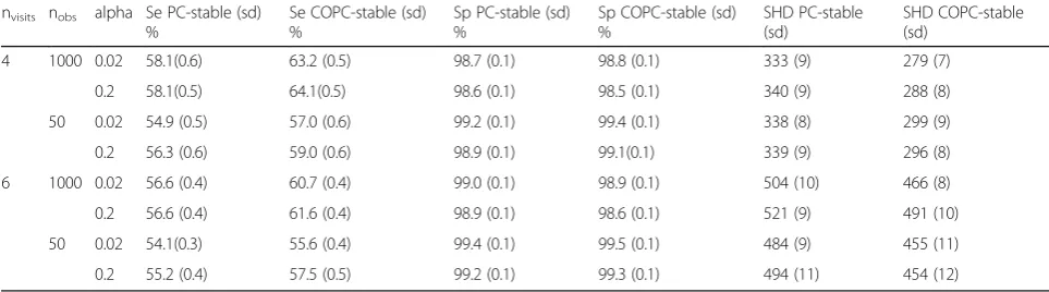
The results of the simulations are presented in Table2.

Overall, COPC-stable outperformed PC-stable in terms of sensibility, meaning that the percentage of false positive was lower in the CPDAGs estimated with COPC-stable rather than the CPDAGs estimated with PC-stable. In terms of specificity, both algorithms showed excellent results. In scenarios with a greater alpha level regarding other parameters, sensibility rose while specificity decreased. By reducing the number of observations from 1000 to 50 we underestimated slightly the sensitivity and specificity.

The COPC-stable SHD was lower than the PC-stable in all scenarios, meaning that, as compared with CPDAGs estimated with PC-stable, CPDAGs estimated with COPC-stable had a structure closer to the true CPDAG (see Table2).

In terms of accuracy, the estimations of causal effects based on CPDAGs estimated with COPC-stable were more accurate than the ones using CPDAGs estimated with PC-stable (see Additional file5for results of all scenarios).

Application

Both IDA and our extension have been applied to our ob-servational data of repeated immunological biomarkers from patients treated with immunotherapy for metastatic melanoma. They have been repeatedly run 300 times on

subsamples of sizen= 30. The tuning parameterαwas set

to 0.02.

As expected, CPDAGs obtained using a naive

PC-stable from unordered repeated measures led to non-chronological ordered paths in all three models

(Fig. 3) as compared with paths identified through

COPC.

Table 1Biological models representing different level of immunological expression

Model Common biomarkers (n) Adaptive T cells immunity biomarkers (n) Total number of covariates

Model 1 Non-immunologic and innate immunological biomarkers (29)

CD4 and CD8 (8) 37

CD4\CD8 expressing polarization and domiciliation markers (148)

177

Subgroup of CD4\CD8 expressing polarization and domiciliation markers (232)

(7)

Table3 shows the average number of edges according to the version of the PC-algorithm and the model. As compared with PC-stable, the percentage of bidirected edges among all edges using COPC-stable was on aver-age smaller in all three models, 100% vs 28% for model 1, 98% vs 40% for model 2 and 97% vs 52% for model 3.

Moreover, Table 3 shows the number of wrongly

defined edges into the final CPDAG. For instance, in model 1, when using a naive approach of the PC-stable, the resulting CPDAG had on average 14 bidirected edges that were between two variables measured at

different times. When looking at Table 4, the number

of values in each multiset Θi also called ambiguity (â)

of the multiset [1] was smaller when using

COPC-stable rather than PC-stable for a same value of

alpha (α= 0.02). The maximum ambiguity reached in

our application was 3.

Estimating time-dependent causal effects in the melanoma example

After estimating the CPDAG using COPC-stable, causal

effects were estimated using Pearl’s do-calculus. To

determine which biomarker had a robust causal effect, we intended to select biomarkers with PCER threshold

≤0.5%. In model 1, there were no biomarkers with a

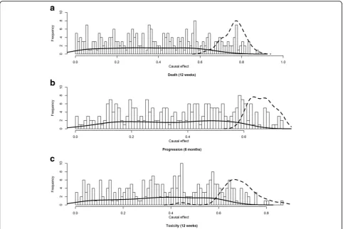
PCER < 0.005. Figures4and5show histograms of causal

effects on our three outcomes death, progression and toxicity based on model 2 and 3. The causal effects seem almost uniformly distributed between 0 and 1 in our example for models 2 and 3. However, immunological biomarkers with a PCER under 0.5% had a causal effect concentrated between 0.6 and 0.8 for models 2 and 3 for all outcomes. On the other hand, causal effects sizes of immunological biomarker with PCER > 0.5% were spread in a wide range from 0 to 1.

Table 2Average sensibility, specificity and SHD according PC-stable and COPC-stable over 500 replicates simulated based on 2 DAGs with different number of visits

nvisits nobs alpha Se PC-stable (sd) %

Se COPC-stable (sd) %

Sp PC-stable (sd) %

Sp COPC-stable (sd) %

SHD PC-stable (sd)

SHD COPC-stable (sd)

4 1000 0.02 58.1(0.6) 63.2 (0.5) 98.7 (0.1) 98.8 (0.1) 333 (9) 279 (7)

0.2 58.1(0.5) 64.1(0.5) 98.6 (0.1) 98.5 (0.1) 340 (9) 288 (8)

50 0.02 54.9 (0.5) 57.0 (0.6) 99.2 (0.1) 99.4 (0.1) 338 (8) 299 (9)

0.2 56.3 (0.6) 59.0 (0.6) 98.9 (0.1) 99.1(0.1) 339 (9) 296 (8)

6 1000 0.02 56.6 (0.4) 60.7 (0.4) 99.0 (0.1) 98.9 (0.1) 504 (10) 466 (8)

0.2 56.6 (0.4) 61.6 (0.4) 98.9 (0.1) 98.6 (0.1) 521 (9) 491 (10)

50 0.02 54.1(0.3) 55.6 (0.4) 99.4 (0.1) 99.5 (0.1) 484 (9) 455 (11)

0.2 55.2 (0.4) 57.5 (0.5) 99.2 (0.1) 99.3 (0.1) 494 (11) 454 (12)

(8)

Tables 5 shows the top effect biomarkers among

those selected for models 2 (see Additional file 6 for

the list of all selected immunological biomarkers). We see that some of the biomarkers are present in all top 10 but differ with the time of measurement. We see that BM30 is present in the top 10 for toxicity at visit 1, in the top 10 for progression at visit 3 and in the top ten for death at visit 4. Other biomarkers are present in 2 of the top 3 but differ with the visit such as BM26, BM45, BM39 and BM9.

Discussion

We extended in this paper the IDA method to repeated measures by introducing a chronologically ordered (CO) version of the so called PC-algorithm. Our proposed algorithm COPC-algorithm takes a priori chronological information, such as repeated measure, into account in the input graph. We then applied PC-stable and our new method COPC-stable to simulated data sets and obser-vational data of repeated immunological biomarkers from patients treated repeatedly with immunotherapy for metastatic melanoma. When comparing CPDAGs obtained with PC-stable and those with COPC-stable, the simulation study showed that PC-stable had a lower sensitivity than the COPC-stable leading to a better learning of the true structure. On the application,

CPDAGs based on PC-stable had indeed

non-chronological ordered paths while those based on COPC-stable could not have any. CPDAGs obtained with COPC-stable had on average more total and directed edges than those obtained with PC-stable but less bidirected edges. The lower the number of directed

edges, the lower the number of possible ways to direct edges, hence the lower the number of DAGs in the

Markov equivalence class. Moreover Table4showed that when using COPC-stable, the proportion of values

obtained in the multiset Θi was on average lower when

using PC-stable. Smaller the Markov equivalence class,

higher the power of the study to identify causal effects. In the COPC-stable, the number of tested conditional dependencies is considerably smaller than with PC-stable. Since it takes chronological order information into account, the COPC-algorithm does not test dependencies of two variables conditioning on a variable measured at a time after those two variables. In contrary, the original PC-algorithm tests non-realistic conditional dependences and thus raises the number of global tests. Testing those non-realistic conditional dependences could lead to identi-fying false positive causal effects.

Finding the true causal DAG has always been the principle interest of causal inference studies, knowing the true causal DAG allows the estimating of the true causal effect. However, in high-dimensional setting, the true causal DAG is generally unknown and it is difficult to check whether or not all possible confounders are measured. Therefore IDA was developed to estimate

lower bounds of the causal effects ofXionYand

deter-mine the importance of these effects. This is a different approach where instead of searching one true causal effect, a range of causal effects are estimated in each

DAG from a Markov equivalence class. Consequently,

when an effect of large numbers of markers is identified, those which have causal effects could be selected by different approaches. In fact, we could either keep a

Table 3Average number of edges (standard deviation) in the CPDAG according to the version of the PC-algorithm and the model over 300 runs with alpha = 0.02

Directed edges (sd) Bidirected edges (sd) Total (sd) Non-chronologically ordered edges (sd)

Naïve PC-stable (model 1) 0 (0.1) 19 (0.1) 19 (0.1) 14 (0.1)

COPC-stable (model 1) 18 (0.1) 7 (0.1) 25 (0.1) 0 (0)

Table 4Probability of having a certain ambiguityâfor biomarkers with an alpha level at 0.02 according to the version of the PC-algorithm (PC-Stable/ COPC-stable) over 300 with alpha = 0.02

Model 1 Model 2 Model 3

Ambiguity PC-stable COPC-stable PC-stable COPC-stable PC-stable COPC-stable

â=1 0.243 0.676 0.153 0.599 0.061 0.437

â=2 0.568 0.297 0.655 0.356 0.693 0.494

(9)

small range of biomarkers that are in the top effects as

in [21] or a larger range of those with a limited but

slightly higher probability of being false positive. In the high-dimensional setting, the first approach will keep biomarkers with the strongest causal effect but not necessarily all biomarkers with a small causal effect. The second approach assures to select a larger list of bio-markers that have a robust causal effect and will suggest to clinicians which immunological biomarkers they should investigate deeper in a follow-up study. Also, controlling for type 1 error can be done by different methods. We chose in our application the PCER because it is less restrictive compared to methods such as FDR (False discovery rate) or FWER (Family-wise error rate).

The choice of the selecting approach depends on the objective: selecting a small list of biomarker that have the highest effect on the outcome or identifying all the biomarkers that have an effect regardless of the size ef-fect. For instance, if only the measure of a marker at visit 2 belongs to the top causal effects, should we only consider the marker at visit 2 or should the marker be measured at all visits? Usually, in a causal DAG, all true causal effects have to be reported, not only the stron-gest. Nevertheless, the interpretation of the top causal

biomarker is challenging. Having a biomarker at a cer-tain visit with a PCER below the selected threshold does not mean that the biomarker has a causal effect only at this visit but rather its maximum and more ro-bust effect at this visit.

One of the main assumptions made in this study is that the true DAG is not dynamic like other

exten-sions of the PC-algorithm on time-series data [28,

29]. So we did not constrain the arrows to be the

same within each visit. In fact, the context of bio-logical biomarkers can be much more complex than a simple repetition of a pattern. Originally, the IDA made the assumption that all variables including the outcome were Gaussian, then it has been extended in a case where all variables (including outcome) are

discrete [14]. In this study we made the assumption

that all covariates X= {X1,…,Xp} are Gaussian and

that the outcome is binary because it is a situation that is quite common in oncology. Also, the covari-ates need to be measured at uniform set of time points (i.e. balanced data).

Our work aimed to find causal effects among re-peated immunological biomarkers on death and tox-icity of patients treated with immunotherapy for

Fig. 4Histogram of the causal effect for the biomarkers on death (a), progression (b) and toxicity (c) based on model 2 over 300 runs. Solid and

(10)

metastatic melanoma. Based on our observational data, using the IDA with our new version of the PC-algorithm, the COPC-algorithm, we found a con-sistent list of immunological biomarkers with causal effects. But one should be attentive not to overinter-pret these results. It is in fact impossible to accurately

check whether or not our assumptions hold; having no unmeasured confounders is a strong assumption but may be reasonable in our application.

Further work will investigate the addition of expert knowledge as input of the COPC-algorithm based on

high-dimensional graphs. Also we will explore

Fig. 5Histogram of the causal effect for the biomarkers on death (a), progression (b) and toxicity (c) based on model 3 over 300 runs. Solid and

dashed lines represent the kernel density of biomarkers with a PCER > 0.5% and PCER≤0.5% respectively

Table 5Top 10 of immunological biomarkers with a PCER < 0.5% in model 2. The number following“v”stands for the visit number. Superscript indicate biomarkers in common. See Additional file3for the complete description of the biomarkers

Death (12 weeks) Progression (6 months) Toxicity 12 weeks

Rank Biomarker Median effect PCER Biomarker Median effect PCER Biomarker Median effect PCER

1 BM16v2a 0.81 0.0035 BM8v1d 0.77 0.0031 BM7v4 0.79 0.0028

2 BM5v1 0.81 0.0035 BM44v4 0.72 0.0036 BM8v4d 0.76 0.0034

3 BM42v3 0.80 0.0037 BM26v2 0.71 0.0041 BM16v3a 0.75 0.0036

4 BM48v1 0.86 0.0037 BM30v3b 0.71 0.0041 BM26v4 0.75 0.0036

5 BM42v2 0.80 0.0038 BM44v3 0.68 0.0042 BM7v3 0.76 0.0037

6 BM14v4 0.79 0.0039 BM45v1e 0.70 0.0047 BM9v4c 0.72 0.0039

7 BM30v4b 0.80 0.0039 BM39v4f 0.66 0.0049 BM39v3f 0.72 0.0039

8 BM11v4 0.83 0.0040 BM40v4 0.66 0.0049 BM32v3 0.71 0.0042

9 BM11v1 0.76 0.0042 BM14v2 0.66 0.0050 BM30v1b 0.67 0.0045

(11)

extensions that can deal with longitudinal and time to event outcomes.

Conclusions

In this paper, we presented an extension of the PC-algorithm called COPC-algorithm. It provides CPDAGs that keep the chronological structure present in the data and allow us to estimate reliable lower bounds of the causal effect of repeated covariates or biomarkers. In the immuno-therapy example, immunological biomarkers on early toxicity, premature death and progression were identified and will be further investigated by clinicians.

Additional files

Additional file 1:Estimation of causal effect. It details the formulas used for the calculation of causal effects. (DOCX 26 kb)

Additional file 2:Simulation setting. It details the process of the generation of the data for the simulation study. (PDF 113 kb)

Additional file 3:Description of biomarkers. It describes the names of the anonymised biomarkers. (DOCX 30 kb)

Additional file 4:Missingness graphs. It details the process used to recover missing data. (DOCX 212 kb)

Additional file 5:Estimation of the Mean squared error. It provides supplementary tables of the simulation study results. (DOCX 27 kb)

Additional file 6:Estimation of biomarkers’median effect. It provides supplementary tables of the application results. (DOCX 31 kb)

Abbreviations

COPC-algorithm:Chronologically ordered PC-algorithm; COPC-stable: Chronologically ordered PC-stable; CPDAG: Completed partially Directed Acyclic Graph; CStaR: Causal Stability Ranking; DAG: Directed Acyclic Graph; FDR: False discovery rate; FWER: Family-wise error rate;

IDA: Intervention calculus when the DAG is Absent; MSM: Marginal Structural Model; PC-algorithm: Peter Clarks -algorithm; PCER: Per comparison error rate; SHD: Structural Hamming Distance

Acknowledgements

Vahé Asvatourian was supported by Université Paris Sud. Clelia Coutzac was supported by fellowships from Fondation pour la Recherche Médicale (FRM). The authors would like to thank Gustave Roussy Cancer Campus, INSERM and INCa for their funding.

Funding

This work is part of a PhD thesis funded by Université Paris Sud. This study was funded by Gustave Roussy Cancer Campus, Fondation Gustave Roussy, the Institut national de la santé et de la recherche

médicale (INSERM), the Direction Générale de l_’Offre de Soins (DGOS;

GOLD TRANSLA 12–174), the Institut National du Cancer (INCa; GOLD

2012_–062 N° Cancéropôle: 2012_–1-RT-14-IGR-01), and SIRIC SOCRATE (INCa

DGOS INSERM 6043), MMO program: ANR-10IBHU-0001). The funding body had no role in the design, analysis, and interpretation of the data, and in the writing of the manuscript.

Availability of data and materials

The National Commission of Informatics and Liberties (CNIL) which is the French data protection authority, does not allow us to make these data publicly available.

Authors’contributions

VA, SM, EM have conceived the statistical work, VA has drafted the manuscript. CC and NC provided immunological data and helped for the immunological interpretation. CR provided clinical data and help for clinical

interpretation. All authors have critically reviewed the manuscript. All authors read and approved the final manuscript.

Ethics approval and consent to participate

Patients were informed of the study and consented to participate. This study

was approved by the Kremlin Bicêtre Hospital Ethics Committee (SC12_–018;

ID-RCB-2012-A01496–37) and all procedures were performed in accordance

with the Declaration of Helsinki. The protocol was validated in routine care in 2012 using a verbal consent.

Consent for publication

Not applicable.

Competing interests

The authors declare that they have no competing interests.

Publisher’s Note

Springer Nature remains neutral with regard to jurisdictional claims in published maps and institutional affiliations.

Author details

1_{Université Paris-Saclay, Univ. Paris-Sud, UVSQ, CESP, INSERM, Villejuif, France.} 2_{Service de Biostatistique et d}_’_{Epidémiologie, Gustave-Roussy, Villejuif, France.} 3

Gustave Roussy, Laboratoire d’Immunomonitoring en Oncologie, and CNRS-UMS 3655 and INSERM-US23, F-94805 Villejuif, France.4_Université Paris-Sud, Faculté de Médecine, F-94276 Le Kremlin Bicêtre, France. 5_{Université Paris-Sud, Faculté de Pharmacie, F-92296 Chatenay-Malabry,} France.6Department of Medicine, Dermatology Unit, Gustave Roussy Cancer Campus, Villejuif, France.

Received: 21 September 2017 Accepted: 20 June 2018

References

1. Maathuis MH, Kalisch M, Bühlmann P. Estimating high-dimensional

intervention effects from observational data. Ann Stat. 2009;37(6 A):3133–64.

2. Spirtes P, Glymour C, Scheines R. Causation, Prediction, and Search.

New York: Springer Verlag; 1993.

3. Pearl J. Causality: Models, Reasoning, and Inference. 2nd ed. Cambridge:

Cambridge University Press; 2009.

4. Robins JM, Hernán MÁ, Brumback B. Marginal structural models and causal

inference in epidemiology. Epidemiology. 2000;11:550_–60.

5. Hernán MA, Brumback B, Robins JM. Marginal structural models to estimate

the causal effect of zidovudine on the survival of HIV-positive men. Epidemiology. 2000;11:561–70.

6. Robert C, Thomas L, Bondarenko I, O_’Day S, Weber J, Garbe C, Lebbe C,

Baurain J-F, Testori A, Grob J-J, Davidson N, Richards J, Maio M, Hauschild A, Miller WH, Gascon P, Lotem M, Harmankaya K, Ibrahim R, Francis S, Chen T-T, Humphrey R, Hoos A, Wolchok JD. Ipilimumab plus Dacarbazine for previously untreated metastatic melanoma. N Engl J

Med. 2011;364:2517–26.

7. Hodi FS, O’Day SJ, McDermott DF, Weber RW, Sosman JA, Haanen JB,

Gonzalez R, Robert C, Schadendorf D, Hassel JC, Akerley W, van den Eertwegh AJM, Lutzky J, Lorigan P, Vaubel JM, Linette GP, Hogg D, Ottensmeier CH, Lebbé C, Peschel C, Quirt I, Clark JI, Wolchok JD, Weber JS, Tian J, Yellin MJ, Nichol GM, Hoos A, Urba WJ. Improved survival with Ipilimumab in patients with metastatic melanoma. N Engl J Med. 2010;363:711_–23.

8. Drake CG, Lipson EJ, Brahmer JR. Breathing new life into

immunotherapy: review of melanoma, lung and kidney cancer. Nat Rev Clin Oncol. 2014;11:24–37.

9. Schadendorf D, Hodi FS, Robert C, Weber JS, Margolin K, Hamid O, Patt D,

Chen TT, Berman DM, Wolchok JD. Pooled analysis of long-term survival data from phase II and phase III trials of ipilimumab in unresectable or metastatic melanoma. J Clin Oncol. 2015;33:1889–94.

10. Garbe C, Eigentler TK, Keilholz U, Hauschild A, Kirkwood JM. Systematic

review of medical treatment in melanoma: current status and future prospects. Oncologist. 2011;16:5–24.

11. Sargent DJ, Conley BA, Allegra C, Collette L. Clinical trial designs for

(12)

12. Buyse M, Michiels S, Sargent DJ, Grothey A, Matheson A, De Gramont A. Integrating biomarkers in clinical trials. Expert Rev Mol Diagn. 2011;11:171_–82. 13. Pearl J. Causal diagrams for empirical research. Biometrika. 1995;82:669–88.

14. Kalisch M, Fellinghauer BA, Grill E, Maathuis MH, Mansmann U, Bühlmann P,

Stucki G. Understanding human functioning using graphical models. BMC

Med Res Methodol. 2010;10:10_–4.

15. Pearl J. Statistics and causal inference: a review. Test. 2003;12:281–345.

16. Kalisch M, Machler M, Colombo D, Maathuis MH, Buhlmann P, Mächler M,

Colombo D, Maathuis MH. Causal inference using graphical models with the R package pcalg. J Stat Softw. 2012;47:26.

17. Maathuis MH, Nandy P. A review of some recent advances in causal

inference. In handbook of big data. Chapman and Hall; 2016.

18. Colombo D, Maathuis MH. Order-independent constraint-based causal

structure learning. J Mach Learn Res. 2014;15:1_–40.

19. Kalisch M, Buehlmann P. Estimating high-dimensional directed acyclic

graphs with the PC-algorithm. J Mach Learn Res. 2007;8:613–36.