R E S E A R C H
Open Access
A photoacoustic image reconstruction method
using total variation and nonconvex optimization
Chen Zhang, Yan Zhang and Yuanyuan Wang
** Correspondence: [email protected] Department of Electronic Engineering, Fudan University, Shanghai 200433, China
Abstract
Background:In photoacoustic imaging (PAI), the reduction of scanning time is a major concern for PAI in practice. A popular strategy is to reconstruct the image from the sparse-view sampling data. However, the insufficient data leads to reconstruction quality deteriorating. Therefore, it is very important to enhance the quality of the sparse-view reconstructed images.
Method:In this paper, we proposed a joint total variation andLp-norm (TV-Lp) based
image reconstruction algorithm for PAI. In this algorithm, the reconstructed image is updated by calculating its total variation value andLp-norm value. Along with the
iteration, an operator-splitting framework is utilized to reduce the computational cost and the Barzilai-Borwein step size selection method is adopted to obtain the faster convergence.
Results and conclusion:Through the numerical simulation, the proposed algorithm is validated and compared with other widely used PAI reconstruction algorithms. It is revealed in the simulation result that the proposed algorithm may be more accurate than the other algorithms. Moreover, the computational cost, the convergence, the robustness to noises and the tunable parameters of the algorithm are all discussed respectively. We also implement the TV-Lpalgorithm in thein-vitroexperiments to
verify its performance in practice. Through the numerical simulations andin-vitro experiments, it is demonstrated that the proposed algorithm enhances the quality of the reconstructed images with faster calculation speed and convergence.
Keywords:Photoacoustic imaging, Image reconstruction, Total variation,Lp-norm,
Nonconvex optimization
Introduction
Photoacoustic imaging (PAI), also known as optoacoustic tomography (OAT) or ther-moacoustic tomography (TAT), is a novel hybrid biomedical imaging modality which combines the strengths of both optical and ultrasound imaging [1-6]. Due to its non-ionizing nature, it has been considered as a promising imaging technique and developed rapidly during the past decade. PAI reveals physiologically specific optical absorption contrast of the biological tissues, which has great potential in clinic applications such as early tumor detection [7,8], vessel imaging [9,10] and brain imaging [11].
PAI is developed based on the photoacoustic effect [1,2], which is a process describ-ing that the imagdescrib-ing tissues absorb the laser energy and convert it into acoustic waves. In this paper, we focus on the computed-tomographic PAI. In this kind of imaging mode, a laser pulse is used to illuminate the imaging tissues from the top. Some of the
laser energy is absorbed and converted into heat, leading to thermoelastic expansion and thus wideband ultrasonic wave emission. The generated photoacoustic signals are then detected by a scanning ultrasound transducer or a transducer array to form im-ages. Based on these detected signals, the optical absorption deposition of the imaging tissues can be calculated by using an image reconstruction algorithm.
In PAI, the reconstruction algorithms have become the vital factor of imaging quality. The PAI reconstruction result benefits a lot from a stable, accurate and efficient algo-rithm. A variety of analytical image reconstruction algorithms have been developed. Re-construction algorithms based on the inverse spherical radon transform have been proposed in both the time-domain [12,13] and the frequency-domain [14,15]. The fil-tered back-projection (FBP) algorithm proposed by Xuet al. is the most popular algo-rithm due to its accuracy and convenience [16,17]. The deconvolution reconstruction algorithm proposed by Zhang et al. has specific advantage under the circumstance of limited-angle sampling and heterogeneous acoustic medium [18,19]. Several investiga-tions have been made to propose the algorithms in plane geometries for imaging with the linear array of transducer [20,21]. The analytical reconstruction methods have advantage in the computational cost and implementation convenience. However, the analytical algorithms fail to keep effective when the sampling points are sparse. The ignorance of measurements noises leads to the severely quality decline in the noisy situation. Those drawbacks above limit the applications of the analytical algorithms and impair their performance. Then the iterative image reconstruction methods are pro-posed to overcome these shortcomings and enhance the image quality of PAI.
Wanget al.with the TV utilized in the iteration [33]. They investigate and employ the TV-based iterative image reconstruction algorithms in three-dimensional PAI. Zhang et al. utilizes the TV coefficient along with the gradient descent method in PAI recon-struction to propose the Total variation based gradient descent (TV-GD) algorithm [34]. The TV-GD method is reported to be stable and efficient under the sparse-view circumstance for PAI reconstruction. From the discussion noted above, it can be de-duced that the iterative algorithms for PAI reconstruction have advantage in recon-struction qualities and robustness to noise. Now the reduction of scanning time is the main concern of PAI. A popular strategy is to reconstruct the image from sparse-view sampling data. Also there exists photoacoustic imaging system which can image the whole area with one laser exposure. These systems usually have large amount of trans-ducers around the imaging area. With the help of sparse-view photoacoustic imaging reconstruction method, the transducer amount can be reduced. This reduction benefits the system from two main aspects. First, it helps to manage the system complexity to a lower level. The lower complexity system is more stable and easier to maintain. Second, this reduction also means the reduction of data scale. The data scale reduction can make the acquisition process more simple and flexible. Besides these two aspects, it is also worth to mention that it reduces the cost of the whole system. All those men-tioned above is very important for further clinical applications. It is very important to develop a sparse-view imaging system. In this situation, the qualities of the iterative re-constructed images have room for improvement. Take the TV-GD method for example, it is reported to be an efficient and high-quality algorithm in sparse-view situation. But the paintinglike artifacts emerge and some detail information is lost in the extremely sparse-view reconstruction.
The compressed sensing theories have been adopted in PAI reconstruction, in which the L1-norm of the signal is minimized to obtain the reconstructed image. Recently, Chartrand reported that by replacing the L1-norm with theLp-norm (0 <p≤1), accur-ate reconstruction is possible with substantially fewer measurements [35]. This noncon-vex optimization setting has been successfully applied to Magnetic Resonance Imaging (MRI) image reconstruction [36,37]. The results show that the algorithm with Lp-norm can provide accurate reconstruction image with fewer measurements comparing to the L1-norm based algorithms. To another dimension of this optimization problem, seve-ral algorithms have been proposed to get a better performance in image reconstruc-tion through jointly minimizes the TV value and L1-norm value [38,39] in MRI image reconstruction.
parameter investigation. Through the numerical simulations and in-vitroexperiments, it is demonstrated that the proposed algorithm enhances the quality of the reconstructed images with the faster calculation speed and convergence. It’s worthwhile to mention that like Ref. [27] and other iteration method, we also used a projection matrix to connect the acoustic pressure measurements with the reconstructed image. But there are some imple-mentation differences between our method and that one. We both use an intermediate variable to simplify our equations. Ref. [27] used the velocity potential as the intermediate variable and we used a linear integration of the initial pressure along an arc whose center is the position of the ultrasound sensor and with a certain radiusct. The Ref. [27] used a sparsifying matrix and minimized the L1-norm in sparsifying domain to get the recon-struction. We used the information from sparsifying domain and piecewise continuous behavior to reconstruct the image. Also, we adapted thep-norm minimization into the al-gorithm, so it can be a more accurate algorithm in sparse-view PAI.
The main contribution of this paper is to develop a novel algorithm for solving the problem of reconstructing the image from sparse-view data in PAI. Our contributions are threefold. First, we include the nonconvex optimization into the PAI reconstruction. This nonconvex optimization setting can provide more stable and accurate result under the sparse-view situation. Second, we combine the nonconvex optimization with TV minimization. The combined method is able to reconstruct more detailed image with sharp edge. Finally, we implement the Barzilai-Borwein method accelerates the recon-struction speed and improves the convergence considerably.
This paper is organized as follows. ‘Theory and method’describes the theory of the proposed algorithm. The numerical simulation is introduced in ‘Simulation’. The in -vitro experimental results are shown in‘In-vitro experiments’. The conclusions of this work are drawn in‘Conclusion’.
Theory and method Photoacoustic theory
In this paper, the two-dimensional PAI is concerned in the simulations and experiments. In 2D PAI, a laser pulse is used to illuminate the imaging tissues from the top. Due to the photoacoustic, the illumination creates an initial acoustical pressure field. The initial acoustical pressure field propagates as ultrasound waves, which can be detected by ultra-sound transducers. Based on the physical principle of the photoacoustic effect, assuming that the illumination is spatially uniform, the relationship between the acoustical pressure measurements and the initial pressure rise distribution can be derived as :
∇2 p r→;t
−1 c2
∂2 p r→;t
∂t2 ¼−
μ
Cpu r
→ ⋅∂I tð Þ
∂t ð1Þ
wherep r→;tis the acoustic pressure measurements at the position r and the timet,
cis the sound speed,Cpis the specific heat,μis the isobaric expansion coefficient,I(t)
is the temporal profile of the laser pulse and u r→ is the initial pressure rise
In order to recover initial data for the wave equation, several inversion formulas have been established to solve this as a filtered back-projection problem [12,40]. By using the Green’s function [12] to solve equation (1), the acoustic pressure measurements can be deduced as:
p r→ 0;t
¼ μ 4πCp
∂ ∂t
∯
r→−→r0
¼ct
u r→
t d
2 r
→ ð
2Þ
where→r
0 is the position of the ultrasound transducer.
In PAI experiments, an ultrasound transducer is used to receive the acoustic pressure measurements at different positions, and the image reconstruction is regarded as an in-verse problem to obtain the initial pressure rise distribution. In the iteration of the image reconstruction, a projection matrix A is typically established to connect the acoustic pressure measurements with the reconstructed image. The measurements can be calculated based on the reconstructed image, and then the reconstructed image can be repeatedly corrected by minimizing the difference between the calculated measure-ments and the real ones. In this way, the optimization method can be used for collabor-ation and then the itercollabor-ation reconstruction algorithm can be developed.
Compressed sensing for PAI
If the sampling data is insufficient, the projection matrixAis ill-conditioned. Thus, the matrix Adoes not have an exact inversion. As a result, it leads to streaking artifacts in the reconstructed image. This problem can be treated by incorporating the compressed sensing theory into PAI.
We define a new variablefas:
f →r 0;t
¼4πCp
μ Z t
0 p r→
0;t
dt⋅t ð3Þ
Then the equation (2) can be converted as follows:
f →r 0;t
¼
∯
jr0−r0j¼ctu r→
d2→r ð4Þ
In practical imaging, the reconstructed image and the measurements are processed discretely, and the image is reshaped into vectors for convenience. If the size of the
re-constructed image u r→ is X pixels ×Ypixels, then the total pixel number of the
re-constructed image u r→ is N (N=XY). After vectorization, the reconstructed image
u r→ becomes a vector u with the length of N. If the total number of the detection
points is Q, the length of measurement in each detection point isM, the equation (4) can be expressed as:
fi¼AiT⋅u i¼1;2;⋯;Q ð5Þ
wherefiis the integration of the u r →
along the arc that is centered inith detection
T is the transpose operation of a matrix. The calculation of the projection matrix is as follows:
(a) Calculate an matrixAi(j) as:
Aið Þ ¼j max 1−d⋅
dx c⋅dt−j
;0
1≤j≤M
ð Þ ð6Þ
whered¼
ffiffiffiffiffiffiffiffiffiffiffiffiffiffiffiffiffiffiffiffiffiffiffiffiffiffiffiffiffiffiffiffiffiffiffiffiffiffiffi m−mi
ð Þ2þ n−n
i
ð Þ2 q
, (m,n) is the position of thejth point in the
recon-structed image,(mi,ni) is the position of the ith detection point,dxis the actual length between the two pixels in the reconstructed image,dtis the discretized time step andM is the total sampling points at one detection point.
(b) Vectorize the matrixAi(j) as thejth column vector in projection matrixAi. (c) Repeat the calculationMtimes to get the projection matrixAi.
(d) Repeat step(a) to step(c)Qtimes to get the projection matrix in the different sampling positions (A1,A2,…,AQ). Then write the projection matrixes in the forms as follows:
A¼ A1T A2T ⋮ AQT
0 B B @ 1 C C
A ð7Þ
The equation (6) can be expressed as:
f ¼A⋅u ð8Þ
where the sizes of f, A and u are MQ pixels × 1 pixel, MQ pixels ×N pixels and N pixels × 1 pixel respectively.
To reconstruct the photoacoustic image from incomplete measurements by using the compressed sensing theory, we can solve an optimization problem as follows:
minu ΨTu 1þ
1
2jAu−fj2
2
ð9Þ
where Ψis a sparse transform matrix,| |1and | |2are theL1-norm and L2-norm re-spectively. By projecting the image onto an appropriate basis set, we can get a sparse representation of the original image. In this domain, most coefficients of the image are small, and a few large coefficients capture most information of the signal. In this way, we can recover a much more accurate image from those undersampled measurements.
In practical applications of PAI, the reconstructed images often show piecewise con-tinuous behavior. The images like this always have small total variation (TV) values, which is defined as follows:
TVð Þ ¼u Z
Du j j ¼XN
i¼1 Diu
j j2 i¼1;2…N ð10Þ
size of 2Npixels ×Npixels, andD =(DX;DY),DX andDYare the horizontal and vertical global finite difference matrixes respectively.
It is reported that the TV based reconstruction algorithm can recover the image ac-curately from sparse sampling data [34]. Using TV values to reconstruct the image can be expressed mathematically as:
minu TVð Þ þu 1
2jAu−fj2 2
ð11Þ
However, the TV minimization still has some limitations that impair its performance. The optimization of the TV value encourages the recovery of images with sparse gradi-ents, thus resulting in the paintinglike staircase artifacts in the reconstructed images.
Recently, some research find out that the nonconvex optimization can reconstruct an accurate image with fewer measurements by replacing the L1-norm with the Lp-norm (0 <p≤1). Aiming to enhance the reconstruction quality and overcome the problem of TV based algorithm, we joint the Lp-norm with TV values to establish a new opti-mization which can be defined by:
minu α⋅TVð Þ þu βΨTuppþ
1
2jAu−fj2
2
0<p≤1 ð12Þ
where α and β are parameters corresponding to the weights of the TV value and Lp-norm value , | |pis the Lp–norm in this optimization problem respectively.
Therefore, we can obtain the reconstructed image by solving this new optimization problem in equation (12).
PAI reconstruction algorithm
In this part, we solve the optimization problem in equation (12) to establish a novel photoacoustic image reconstruction algorithm by using the total variation and noncon-vex optimization.
We define the finite difference approximations to partial derivatives of u at the ith pixel along the coordinate as variable ωi=Diu, theith pixel’s sparse coefficient as vari-able zi=ΨiTu, where Ψi is the sparse transform matrix of the ith pixel. The equation (12) can be deduced as:
minu;z;ω α
X
i
ωi
j j2þβ
X
i
zi j jp
pþ
ρ
2jA⋅u−fj
2 2
( )
i¼1;2…N ð13Þ
where ρis the parameter corresponding to the weight of the constraint condition in this optimization problem.
We form the augemented Lagrangian defined by
L ω;z;u;bk;ck
¼αX
i
ωi j j2þ
ρ
2 ωi−Diu k−bk
i
2
2
þβX
i
zi j jp
pþ
ρ
2 zi−Ψ
T
iuk−cki
2
1
þ1 2jA⋅u−fj
2 2
ð14Þ
This problem can be solved by
ωkþ1;zkþ1;ukþ1
¼ minω;z;uL ω;z;u;bk;ck
; bikþ1¼bki− ωikþ1−Diukþ1
; ckiþ1¼cki− zkiþ1−ΨTiuk
; 8 > < >
: ð15Þ
where ωk+1 is the finite difference approximations to partial derivatives of u in (k+ 1)th iteration,zk+1is the sparse coefficient in (k+ 1)th iteration, uk+1is the vector-ized image reconstruction in (k+ 1)th iteration,zik+1is the sparse coefficient of theith pixel in (k+ 1)th iteration, ωik+1 is the finite difference approximations to partial de-rivatives of u at theith pixel along the coordinate in (k+ 1)th iteration;bik+1is the TV step parameter in (k+ 1)th iteration, cik+1 is the Lp-norm step parameter in (k+ 1)th iteration.
By using the standard augmented Lagrangian method, the optimization problem in (15) can be deduced as
ωkþ1;zkþ1;ukþ1
¼ minω;z;u α
X
i
ωi j j2þ
ρ
2 ωi−Diu k−bk
i
2
2
þβX
i
zi j jppþρ
2 zi−Ψ
T
iuk−cki
2
1
(
þδk
2 ω
kþ1−ωk
2
2þz kþ1−
zk
2
2þu−u
kþδ−1
k A
T
Auk−f
2
2
)
ð16Þ
where ωk is the finite difference approximations to partial derivatives of u in kth iteration, zk is the sparse coefficient in kth iteration, uk is the vectorized image reconstruction in kth iteration; δk is the Barzilai-Borwein step parameter in kth iteration.
After using the Barzilai-Borwein method to determine the step size δ, the optimization problem in equation (13) can be transformed into three sub-problem as follows:
ωkþ1
i ¼ minωi j jωi2þ
ρ
2 ωi−Diu
k−bk i
2
2þ
δk
2α ωi−ω
k i 2 2 ;
zkiþ1¼ minzi j jzi
p pþ
ρ 2 zi−Ψ
T iuk−cki
2
1þ
δk
2β zi−z
k i 2 2 ;
ukþ1¼ min
u αρDu−ωkþ1 2 2þβρ Ψ
Tu− zkþ1
2
2þδk u− uk−δ −1
k AT Auk−f
2 2 n o ; bikþ1¼bki − ωikþ1−Diukþ1
; ckiþ1¼cki − zkiþ1−ΨTiuk
; δkþ1¼ A ukþ1−uk
22=
ωkþ1−ωk
2
2þz kþ1−zk
2
2þu kþ1−uk
2 2 8 > > > > > > > > > > > > > < > > > > > > > > > > > > > :
ð17Þ
where ωik is the finite difference approximations to partial derivatives of u at the ith pixel along the coordinate in kth iteration respectively, zik is the sparse coefficient of the ith pixel in kth iteration respectively; δk+1 is the Barzilai-Borwein step par-ameter in (k+ 1)th iteration.
ωikþ1¼ max a1t1þa2t2 a1þa2
− 1
a1þa2;
0
1=
a1þa2
ð Þ
1=ða1þa2Þ
k k
a1¼Diukþbik a2¼ωik t1¼ρ t2¼δk=α
i¼1;2…N
ð Þ 8 > > > > > > < > > > > > > :
ð18Þ
wherea1,a2,t1andt2are the variables used for a succinct expression.
As for the z-subproblem in equation (17), we use the soft p-shrinkage operator to solve it. The operator is defined by:
zikþ1¼ max a
3t3þa4t4
a3þa4
− 1
a3þa4
a3t3þa4t4
a3þa4
1−p;0
( )
1=ða3þa4Þ
1=ða3þa4Þ
k k
a3¼ΨiTukþcik
a4¼zik
t3¼ρ
t4¼δk=β
i¼1;2…N
ð Þ 8 > > > > > > > < > > > > > > > :
ð19Þ
wherea3,a4,t3andt4are the variables used for a succinct expression.
The u-subproblem in equation (17) is a typical least squares problem. The solution can be easily obtained by:
ukþ1¼FT F αρD
Tωkþ1þβρΨTzkþ1þδ
kuk−A−1 Auk−f
αρFTDTDFþβρIþδkI
ð20Þ
whereFis the Fourier transform matrix.
As a result, theTV-Lpalgorithm is summarized as follows:
(1) Initialization: inputf,α,β,ε,pandρ. Set the reconstructed image u0= 0,b = c= 0,
δ0= 1,k= 0.
(2) Apply equation (18) and (19) to update the value ofωandz. (3) Apply equation (20) to update the value of u.
(4) Apply equation (17) to update the value ofb,candδ.
(5) If the exiting condition is met, end the iterations and output the result. Otherwise repeat the step from (2) to (4). The exiting condition is as follows:
uk−uk−1
uk
k k <ε ð21Þ
Simulation
Sparse-view reconstruction
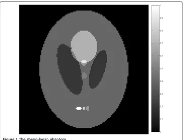
In the simulation, we choose the Shepp-Logan phantom to be the initial pressure rise distribution. The forward simulation and inverse reconstruction are all performed in 2D. The phantom is shown in Figure 1. The measurements from the phantom are gen-erated by using equation (2). The size of the phantom is 89.6 mm × 89.6 mm, the radius of the scanning circle is 42 mm and the size of the reconstructed image is 128 pixels × 128 pixels. During the simulation, the scanning circle covers 360°around the imaging phantom. Four different measurements are collected. The scanning step of tomo-graphic angels is set to 2.25°, 4°, 12° and 20° respectively. So the sampling points are 160 views, 90 views, 30 views and 18 views correspondingly.
The parameters α, β, ε and ρare set to be 1 × 10⁻², 1 × 10⁻², 1 × 10⁻⁵and 1 respec-tively. The influence of these parameters will be discussed later. And the parameter p are set to be two different values as 0.5 and 0.8.
We choose the FBP [16], theL1-norm [27] and the TV-GD [34] algorithms to be the comparison besides our proposed TV- Lp algorithm. The simulation results by using these different algorithms are shown in Figure 2. It’s worthwhile to note that the weight used in the TV-GD algorithm is an adaptive parameter, as same as it is reported in [27]. The negative values in FBP reconstructed image are set to be zero.
It is shown in the first column of Figure 2 that, all three iterative algorithms have comparable reconstruction results when the sampling data is sufficient. Moreover, it is shown in Figure 2(a) that the contrast of FBP reconstructed image is not as high as the other three. But its resolution is comparable with the others visually. When the number of sampling points reduces, the qualities of the reconstructed images are strongly affected in the FBP reconstruction. When the sampling point gets sparse in the FBP reconstruction, the arc-like artifacts appears due to the back-projection arcs
cannot be canceled out with each other. The iterative algorithms can provide better qualities of the reconstructed images than the FBP method in sparse-view reconstruc-tions. Among them, the L1-norm method struggles to depress the noise. Meanwhile, the TV-GD algorithm and the TV-Lp algorithm provides high-resolution images and have no visually distinguishable decline in qualities of the reconstructed images as the number of sampling points decreases.
As for the extreme sparse sampling points situation (18-view and 30-view), the image reconstructed by the FBP algorithm, shown in Figure 2(d), has extremely severe artifacts. TheL1-norm reconstruction and the TV-GD algorithm have a decline in image qualities. The noise in the reconstructed images by the L1-norm reconstruction, as shown in Figure 2(j), cannot be depressed effectively. As for the TV-GD algorithm, the reconstruc-tion produces piecewise artifacts which also make the qualities of the reconstructed
Figure 2The shepp-logan phantom reconstruction results by different algorithms.The first to fifth rows refer to the FBP(a-d), L1-norm(e-h), TV-GD(i-l), TV-Lp (p = 0.5)(m-p)and TV-Lp (p = 0.8)(q-t)
images decrease. In the TV-Lpimage, the noise is depressed more effectively than the above three algorithm. The quality of the reconstructed image is not affected substantially by the insufficient sampling data.
We calculate the peak signal-to-noise ratios (PSNR) of the reconstructed images with the original phantom as a gold standard to provide a numeric quantification of the re-sults. The bigger the value of PSNR is, the better quality of the image is. The PSNR is defined as:
PSNR¼10 log10 XY⋅MAX
XX;Y
i;j
ð Þ¼1
u ið Þ;j −t ið Þ;j
ð Þ2
0 B B B B B @
1 C C C C C
A ð
22Þ
where t(i,j) means the gray-value of the original image, MAXthe maximum possible pixel value of the image which in our simulation is 1.
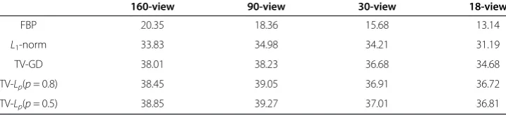
We calculate the value of the PSNR of all images in Figure 2. The quantitative results are shown in Table 1.
From Table 1, it is shown that the PSNR of the FBP algorithm is always in a very low level due to its unsuitability for sparse-view sampling condition. As for those three compressed sensing based algorithms, the PSNR value of images reconstructed by the TV-Lpalgorithm are the highest. The Lp-norm optimization constraint can provide the better performance in the extremely sparse sampling. With this improvement, the TV-Lp algorithm is more accurate than other algorithms in the sparse-view sampling condition shown in the quantitative results. Between the two different value of p, the parameter pthat is set to be 0.5 has a slightly advantage against the other one. Also it is revealed from Table.1 that the 90-view shows higher PSNR than 160-view. When the sampling points are sufficient, it is possible that the fewer-view projection can produce better reconstruction results. But their PSNR is very close with same algorithm. It is fair to say that the results are on the same level of image quality.
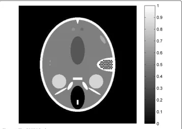
From Figure 2, it is shown that the TV-GD image and the TV-Lpimage are very close in the image quality. Here we choose the FORBILD phantom [41], a more complicated and more challenging phantom, to further compare the proposed algorithm with the TV-GD algorithms. The phantom is shown in Figure 3. The scanning step of tomo-graphic angels is set to 2.25°, 4°, 6° and 12°. So the sampling points are 160 views, 90 views, 60 views and 30 views correspondingly. The other numerical implementation conditions remain the same with the shep-logan simulation. The simulation results by using the TV-GD algorithms and the proposed TV-Lpalgorithm are shown in Figure 4. It is shown in Figure 4 that, when the sampling data is sufficient, both algorithms can
Table 1 PSNRs (dB) of reconstructed images of shep-logan phantom
160-view 90-view 30-view 18-view
FBP 20.35 18.36 15.68 13.14
L1-norm 33.83 34.98 34.21 31.19
TV-GD 38.01 38.23 36.68 34.68
TV-Lp(p= 0.8) 38.45 39.05 36.91 36.72
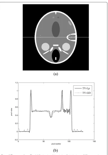
Figure 3The FORBILD phantom.
Figure 4The FORBILD phantom reconstruction results by different algorithms.The first to the third rows show images reconstructed by the TV-GD(a-d)and TV-Lp algorithm with p = 0.8(e-h)and p = 0.5
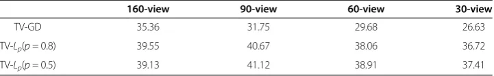
reconstruct the accurate image. When the sampling angles get sparse during the simu-lation, it is seen that the TV-GD reconstruction results in paintinglike staircase artifacts in the smooth regions. Also it fails to give the accurate image in the low contrast re-gions in the top and left of the phantom. The proposed algorithm provides reasonably good reconstructions in these regions. The PSNR of the reconstructed images are shown in Table 2. From this table, we observe that the TV-Lpalgorithm provides the better PSNR for all the cases. In the case of more complicated phantom, the TV-Lp al-gorithm shows significant improvement than the TV-GD alal-gorithm.
Also, we include a line-plots image of the reconstruction result by the TV-GD algo-rithm and the TV-Lp(p= 0.8) algorithm from 30-view data. The location of the pixel profile in the image is displayed in Figure 5(a). The comparisons of pixel profiles are displayed in the Figure 5(b).
In Figure 5(b), the solid line and the dotted line represent the pixel profiles of the TV-Lp and the TV-GD image respectively. It is shown in Figure 5(b) that the TV-Lp can reconstruct the image more precisely than the TV-GD one. The edges from the TV-Lpare sharper than that from the TV-GD. The pixel number from 90 to 100 is the high resolution area, the TV-Lpimage shows the high-speed change of the pixel value while the TV-GD fails to do so. In the continuous area, the TV-Lpimage is smoother.
We continuously decrease the number of the detect points try to find the limit dens-ity of the sampling points. During the simulation, we set the criterion of acceptabildens-ity that the PSNR of the reconstructed image reaches 30 dB. It is found out that the total number of the sampling points is able to be reduced to 15 for TV-Lpalgorithm in the reconstruction of shep-logan phantom and to 18 for the forbild phantom.
In this part, the TV-Lp algorithm is proved to be more accurate and stable than the other algorithms for PAI image reconstruction in the sparse sampling condition.
Convergence and calculation
In this part, we discuss the theoretical calculation complexity and study the conver-gence of the proposed algorithm. As mentioned above in ‘Theory and method’, in step (2) the update of ω and zis using the soft shrinkages and the computational costs are both O(N). The update of z also includes a wavelet transforms which computational costs are O(NlogN). In step (3), the update of u involves two fast Fourier transforms which computational costs are O(NlogN) and two operations of A with the computa-tional costs ofO(NMQ). The update of the parametersbandcin step (4) are all simple calculations with the computational costs of O(N). As for the paremeterδ, although it involves an operation ofA, it can use the result computed in the step (3). So its compu-tational cost is alsoO(N).
In a nutshell, the calculation complexity of the proposed algorithm in one iteration is 5O(N) + 4O(NlogN) + 2O(NMQ). The first two terms is much smaller than the last term in the practical use of photoacoustic imaging and most iterative algorithm is with
Table 2 PSNRs (dB) of reconstructed images of FORBILD phantom
160-view 90-view 60-view 30-view
TV-GD 35.36 31.75 29.68 26.63
TV-Lp(p= 0.8) 39.55 40.67 38.06 36.72
the operation. In each iteration, we just use the projection matrix twice. So the pro-posed algorithm has a cheap per iteration computation.
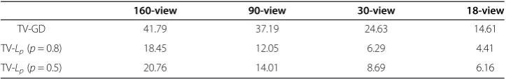
The TV-GD algorithm is reported as an efficient and stable iterative algorithm in photoacoustic imaging. In the ‘Sparse-view reconstruction’, its reconstruction result is closest to the proposed algorithm. So here we select it to be a comparison with the TV-Lpalgorithm. We calculate the time cost of those two algorithms in a simulation. The simulation condition is same as in ‘Sparse-view reconstruction’. But the iteration
ends when the PSNR values reach 30 dB. The result is shown in Table 3. From Table 3, it is shown that the proposed algorithm is faster than TV-GD algorithm in the compu-tational time. Based on this result, it could be inferred that the TV-Lp algorithm is a more efficient image reconstruction algorithm comparing to the TV-GD algorithm. The value ofphas also some influence on the time cost. The smaller thepis, the more iteration times are needed to reach the reconstruction result.
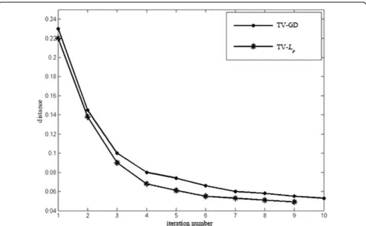
Thanks to the use of Barzilai-Borwein step size selection method, the convergence speed can also be significantly improved. For the quantitative analysis, we use a param-eter that represents the distance between the reconstructed image and the original phantom image. The parameterdis defined as:
d¼
XX
i¼1
XY
j¼1
u ið Þ;j −t ið Þ;j
ð Þ2
XX
i¼1
XY
j¼1 t ið Þ;j2
0 B B B B B @
1 C C C C C A
1=2
ð23Þ
whereuis the reconstructed image andtis the original image. The size of the image is X×Y. The smaller the parameterdis, the closer the reconstructed image is with the original phantom. In the TV-Lp algorithm, there is a small rate of chance that the optimization will lead to the wrong solution due to its non-convex nature. So we use the original image to calculate the parameter dto show the image quality and use the parameter das a reference. We want to show the improvement of the image quality in every iteration step.
The simulation condition is set to be the same as in ‘Sparse-view reconstruction’. The sampling view is 60. The parameterpis set to be 0.8. The defined distancedis cal-culated after each iteration step. If the distance is smaller than 0.05, the iteration will stop. The simulation result is shown in Figure 6. Thex-axis is the value of distance and they-axis is the iteration times. The line‘·-’refers to the TV-GD algorithm and the line
‘*-’represent the TV-Lp(p= 0.8)algorithm. The result is shown in Figure 6. The images reconstructed by TV-Lp algorithm in each iteration have smaller value of d than the TV-GD ones and the TV-Lp iteration only takes 9 times as the distance is met the request.
For discussions noted above, it can be surmised that the convergence of TV-Lp algo-rithm is faster and the TV-Lphas a cheaper computational cost.
Robustness to the noise
In the practical applications of the photoacoustic tomography, the measurements are usually polluted by those white measuring noises from the ultrasound transducer and the system electronics. Hence, it is very important for an algorithm to maintain stable performance under the noises polluted circumstances. To analyze the robustness of the
Table 3 Time cost(second) of reconstructed images
160-view 90-view 30-view 18-view
TV-GD 41.79 37.19 24.63 14.61
TV-Lp(p= 0.8) 18.45 12.05 6.29 4.41
TV-Lpalgorithm, we choose 30-view simulated photoacoustic signals that we used in ‘Sparse-view reconstruction’. The signals are added with white noises of different noise power levels. We use TV-Lpalgorithm with two different settings of parameterp(p= 0.5 andp= 0.8) and TV-GD algorithm to reconstruct images from these white noise polluted measurements.
The reconstruction results are shown in Figure 7. In the first row to the last row of the Figure 7, the signal to noise ratio (SNR) of the polluted measurements is 10 dB, 5 dB, 3 dB and 0 dB, respectively. As shown in the image, when the power level of the noises is not very strong (10 dB and 5 dB), the reconstructed images by using the noisy measurements have basically no obviously difference with the ones reconstructed with the noiseless signals. As the noise becomes stronger, the quality of the reconstructed images decreases.
We also plot the profiles of a pixel line in order to show the detail qualities of recon-structed images clearly. In Figure 7, the dotted line and the solid line are the pixel pro-files of the reconstructed image and the original image, respectively. From the line plots, it is revealed that the proposed algorithm has better performance in the edge preservation and more accurate in the smooth area. We calculated the PSNR of the re-constructed image. The result is shown in Table 4. Our algorithm outperformed the TV-GD algorithm in any noise power level. Giving the credit to the optimal conditions, the reconstructed image is intended to be continuous and sharp. During the iteration, the photoacoustic signals get enhanced and the noise is suppressed.
As we can see from the table that the TV-Lpalgorithm reconstructed images have a slightly better performance than the TV-GD algorithm when it comes to the image qualities. When the noise is extremely strong (0dB), the TV-Lp algorithm has a huge advantage than the TV-GD one in image quality. As for the different settings of para-meterpin the TV-Lpalgorithm, there is no major difference that can be observed be-tween the two images. The PSNRs of thep= 0.5 setting is about 0.3 dB bigger than the
p= 0.8 setting in the first three noise power level. But when the noise getting extremely strong (0 dB), thep= 0.8 setting is 0.1 dB bigger than thep= 0.5 setting in PSNR value. From this part of simulation we can conclude that our TV-Lpalgorithm is robust to noise and has a better performance than the TV-GD algorithm in the noisy measure-ment circumstance.
Parameter investigation
As the original optimization problem of the image reconstruction is described in Eq. (14), the TV-Lpalgorithm contains some parameters that are tunable, which areα,β,ε,
p and ρ. In those parameters, the choice of ρ does not affect the performance of the Figure 7The reconstruction results from noisy signal.The first to the third columns show images reconstructed by the TV-GD(a-d)and TV-Lp algorithm with p = 0.8(e-h)and p = 0.5(i-l), respectively, from signals with SNR of 10 dB, 5 dB, 3 dB and 0 dB.
Table 4 PSNRs (dB) of the noise simulation image
10 dB 5 dB 3 dB 0 dB
TV-GD 32.24 28.01 22.44 16.96
TV-Lp(p= 0.8) 35.14 30.13 27.95 25.21
TV-Lpalgorithm theoretically. The result of the simulation also shows that the image quality is not sensitive to the parameterρfor a large range. Here we set the parameter ρto a steady value 1. Theεis the exiting condition parameter. It can be easily deduced that smaller ε will leads to slightly more accurate reconstructed image at the cost of more iteration times. In this part we focus on analyzing the parameter settings of p,α andβ.
Parameter setting of p
In the TV-Lpalgorithm, we replace theL1norm with theLp norm (0 <p≤1). It is ported in Ref. [35] that theoretically fewer measurements are required for accurate re-construction in the Lp norm situation. But it also leads to failure in solving the optimization problem. It’s kind of a dilemma for the setting ofp. So here we take differ-ent values of pto see its influence to the image reconstruction. The parameterαandβ are both set to be 1 × 10⁻².
We choose the 90-view and 18-view simulated photoacoustic signals that we used in
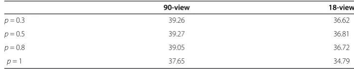
‘Sparse-view reconstruction’. We set thepvalue as 0.3, 0.5, 0.8 and 1. We calculate the reconstructed images’ PSNR value. It is shown in Table 5. When thepis set as 0.5, it has advantage in the quality of the reconstructed image. However, when the value of p continues to reduce to 0.3, there is no obvious improvement in image quality. But in the same time, the smaller thepis, the higher probability of the solving failure is dur-ing the simulation. The reduction of pleads to the increasing of the iteration times in our simulation. So taking these two factors into account, we set the pas 0.8 so that it can provide a great reconstruction performance and stability with a fast convergence.
Parameter settings ofαandβ
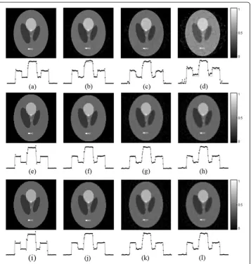
As we describe above in Eq. (14), the parameterαand βare parameters corresponding to the weights of TV value and Lp norm value in this optimization problem respect-ively. We use these two parameters to balance the terms of the objective function. With different kinds of the objective image, the settings of those two parameters are differ-ent. Here we select three different images as the given optical energy deposition to test the universality of our algorithm and present further investigation of the parameter set-tings. We select a phantom that stand for the vessels and a phantom of dots with dif-ferent energy degree in the simulation. We also choose a real brain MRI as the original optical energy deposition to demonstrate the performance of the proposed algorithm in reconstructing extremely detailed and complex structured imaging object. Here the TV-GD algorithm is used as a comparison. There are four groups of parameter settings, which are (α= 1 × 10⁻², β= 5 × 10⁻³) , (α= 1 × 10⁻², β= 1 × 10⁻²), (α= 5 × 10⁻², β= 5 × 10⁻³) and (α= 5 × 10⁻³,β= 5 × 10⁻³). The reconstructed images are shown in Figure 8. From first row of Figure 6, we can see in the reconstruction of gradient sparse phantom.
Table 5 PSNRs (dB) of reconstructed images with differentp
90-view 18-view
p =0.3 39.26 36.62
p= 0.5 39.27 36.81
p= 0.8 39.05 36.72
The TV based algorithm has great performance when the image demonstrate piecewise continuous behavior. All reconstructions are accurate and the background noise is sup-pressed well. When it comes to the images with the vessel phantom (Figure 8 (g)-(l)), those original optical energy depositions are a little bit more complex than the dots. The reconstruction results show that the image reconstructed by TV-Lp algorithm is better than the TV-GD ones. As in Figure 8(h), TV-GD image has some noises in the back-ground and the edge of the vessel is blurred. While the TV-Lpimages with different par-ameter settings both have high-resolution results. As for the real MRI image, it has very detailed information. As expected, both two groups of parameter setting α=β have the most accurate result among them. The increasing weighting of Lp-norm condition can provide more detail information and prevent the reconstructed image emerging plantlike artifacts. The details such as edges and fine structures are well preserved in both recon-structions. The reconstruction results show that the TV-GD reconstructed image has se-verely paintinglike staircase artifacts with some loss in fine details. From our observation, TV-Lpalgorithm with the parameter settingα=βpreserves the fine features better than the TV-GD one. α and β are the regularization parameters determining the trade-off between the data consistency and the sparsity. It is revealed from the above simulation that the parameter settingα=βis a better strategy. In this parameter setting, the TV-Lp algorithm provides a 3 dB improvement in the PSNR over the TV-GD algorithm based on our calculation.
Limited-view and irregular-view simulation
In the real application of PAI, due to the restrains of the shape or the size of the imaging object, a full angular scanning sometimes is hard to achieve. We evaluate the performance of the TV-Lp method in limited-view case, line-view case and un-equal-view case.
Figure 8The different image objectives reconstructed by TV-GD and TV-Lp algorithms.The first to sixth rows refer to the original phantom(a, g, m), the TV-GD reconstructed images(b, h, n), the TV-Lp reconstructed images with parameter settings as (α= 1 × 10⁻²,
β= 5 × 10⁻³)(c, i, o), (
α= 1 × 10⁻²,
β= 1 × 10⁻²) (d, j, p), (α= 5 × 10⁻²,
β= 5 × 10⁻³)(e, k, q)and (
α= 5 × 10⁻³,
The simulation setup and the reconstructed image is shown in Figure 9. In the limited-view simulation (Figure 9(a)), the scanning angular range is set to 150° and the angular step is 3°, so 50-view photoacoustic signals are obtained. In the line-view simu-lation (Figure 9(c)), the transducer array with 60 transducers is placed in the right side of the imaging object and the interval between two transducer elements is 1.49 mm. It
is revealed in Figure 9(b) and Figure 9(d) that the quality of the TV-Lpreconstruction is not much affected by the limitation of the sampling angle. Because the sampling angle is limited, the information definite is partly missed, yet the TV-Lp method can still provide a satisfying reconstruction. In un-equal angel step scanning, we randomly choose 30 sampling points from a 60-view projection and use these 30-view un-equal angle step data for image reconstruction. The result is shown in Figure 9(f ). As we can see from the image, the reconstruction result can still maintain a very high quality.
In-vitroexperiments Experiment setup
We carry out the experiments on in-vitro signals to demonstrate the proposed TV-Lp algorithm’s performance in the practical application.
The framework of the experiment platform is shown in Figure 10. In this platform, an Nd:YAG laser generator (Continum, Surelite I) is used to emit the laser pulse. The wavelength of the laser is 532 nm. A single laser pulse is generated at the frequency of 10 Hz and last 6-7 ns. The incident laser pulse is emitted towards the top of the phan-tom through a concave lens with the diameter of 5 cm. The setup of the lens enlarges the illumination area and lead to the pulse energy reduction in the illumination area. The energy is about 6.47 mJcm−2, which is lower than the ANSI laser radiation safety standard (20 mJcm−2) [1]. Signal acquisition is done by a water-immersion ultrasound transducer (Panametric, V383-SU). The transducer is a linearly unfocused one at 3.5 MHz (-6 dB bandwidth at 45%). A digital stepping motor (GCD-0301 M) is used to ro-tate the ultrasound transducer around the phantom placed in water. The scanning ra-dius is 38 mm. The received analog ultrasound signals are amplified by a pulse receiver (Panametric, 5900PR). An oscilloscope (Agilent, 54622D) with the sampling frequency of 16.67 MHz is set to transform the received signals into digital ones. Both the laser gen-erator and the digital motor are controlled by the computer through the serial interface.
The transformed digital data is transported to the computer through the general purpose interface bus (GPIB).
The imaged phantom we used in the experiment is made by gelatin cylinder. It is shown in Figure 11. There are two different phantoms. The radius of the phantom is 25 mm. The left one is made by two rubber bars with 1 mm diameter that embedded as the optical absorbers. The right one utilizes leaf which pretends as vein and tissue as the optical absorbers.
In the experiment, the transducer tends to measure the photoacoustic signal in-plane only, and the reconstruction is also in 2D. The cross-sectional image in any plane is mainly determined by the measured data in the same plane, and a set of circular meas-urement data on the same plane would be sufficient to reconstruct a good image. We use the deconvlution calculation before the reconstruction to eliminate the transducer’s impulse response influence.
Experiment result
In the experiment, 90-view and 30-view data are collected for reconstruction. The im-ages are constructed by the FBP, the TV-GD and the TV-Lp algorithms, respectively. The reconstruction results are shown in Figure 12. The left column of the Figure 12 is reconstructed from 90-view data. When the sampling data is sufficient, all three algo-rithms are effective. With respect to the locations and sizes, the optical absorbers are all well reconstructed in the figure. While the FBP reconstructed image is not as clear as the images reconstructed by the iterative algorithms. When we reconstruct the image with a small of sampling angles (right column of Figure 11), the artifacts start to emerge in the FBP reconstructed image and the quality of the image is severely af-fected. But the TV-GD and the TV-Lpalgorithms can still provide high-contrast images with less noise. In Figure 12(f ), it is shown that the image reconstructed by the TV-Lp algorithm outperforms other algorithms in image contrast and noise suppression. The structure of optical absorbers is clear and the noise in the background is well-suppressed. The sparse-view of sampling has barely any influence on the quality of the TV-Lp reconstructed image.
In vitro imaging of a leaf vein is also performed to further demonstrate the advan-tages of the TV-Lpalgorithm. The reconstruction result is shown in Figure 13. As the
structure of the phantom is more complex, the FBP are deeply influenced by the ar-tifact and fail to reconstruct the accurate image both under 90-view and 30-view sam-pling circumstance. It is shown in the figure, that the TV-GD and TV-Lp algorithms can still reconstruct the image in a high contrast level. But when the data is insufficient, there is some noise emerging in the background. TV-Lpalgorithms can suppress the noise better than the TV-GD one. The optical absorber in TV-Lpone is more distinct than that in the image by TV-GD algorithm.
Quantitative comparisons
We use the L1-norm algorithm to reconstruct the image of 180-view data from the leaf vein phantom. As the sampling view is efficient, the reconstructed image is used as a
“standard”one. We calculate the histograms of the difference between the reconstructed Figure 12The rubber phantom reconstruction results from experiment data.From left to right, the reconstructed images of rubber sample from 90-view and 30-view experiment data respectively. The first to third rows refer to the images reconstructed by the FBP(a, b), the TV-GD(c, d)and the TV-Lp(e, f)
one and the“standard”one as shown in Figure 14. Figure 14 (a)-(c) are the difference his-tograms between the standard and the images reconstructed by the FBP, the TV-GD and the TV-Lp, respectively, with 30-view data. In Figure 14, two CS-based algorithms have a large number of pixels with small ranges of difference with the standard one, which sug-gests that these two algorithms can reconstruct the image more accurately. In the case of the TV-Lpalgorithm, the major part of the pixel difference is in the range from 0 to 0.1.
Figure 13The leaf vein phantom reconstruction results from experiment data.From left to right, the reconstructed images of leaf vein phantom from 90-view and 30-view sampling experiment data respectively. The first to third rows refer to the images reconstructed by the FBP(a, b), the TV-GD(c, d)and the TV-Lp(e, f)
From this experiment, the results demonstrate that the TV-Lpmethod can outperform the TV-GD one in the field of the image quality.
From the experiment result noted above, it is safe to say that the TV-Lp algorithm would have better performance in sparse-view PAI than other algorithms. It could pro-vide stable and accurate reconstruction in both sufficient data sampling and sparse-view sampling situation.
Conclusion
Aiming to reduce the scanning time and enhance the imaging quality of the photo-acoustic image reconstruction, we proposed the TV-Lpalgorithm that applies the total variation method and nonconvex optimization method to the PAI. The main idea of the algorithm is to apply Lp-norm nonconvex optimization along with the total var-iation method. In the proposed algorithm, the Barzilai-Borwein step size selection method is adopted to provide faster convergence and smaller calculation. The effective-ness and universality of the algorithm is demonstrated through the numerical simula-tions. The numerical simulations show that the TV-Lpalgorithm provides good imaging quality in sparse-view sampling situation. The algorithm convergence, the robustness to noise and the tunable parameters are also discussed. The simulation result reveals that the TV-Lpalgorithm is a stable image reconstruction method with fast convergence and small computational cost. The TV-Lpalgorithm is further investigated through some ex-periments using gelatin-made phantom. Compared with the result of other popular image reconstruction method, the TV-Lp imaging algorithm has significant advantage on con-trast and noise suppression. From the discussion noted above, it could be concluded that the TV-Lpalgorithm may be a practical algorithm for sparse-view photoacoustic imaging reconstruction.
Abbreviations
PAI:Photoacoustic imaging; TV-Lp: Total variation andLp-norm; OAT: Optoacoustic tomography; TAT: Thermoacoustic
tomography; FBP: Filtered back-projection; TV: Total variation; TVM: Total variation minization; ASD-POCS: Adaptive steepest-descent-projection onto convex sets; TV-GD: Total variation based gradient descent; MRI: Magnetic resonance imaging.
Competing interests
The authors declared that they have no competing interests.
Authors’contributions
Study concept and design (CZ); drafting of the manuscript (CZ); critical revision of the manuscript for important intellectual content (CZ, YZ and YW); obtained funding (YW); administrative, technical, and material support (CZ and YZ); study supervision (YW). All authors read and approved the final manuscript.
Acknowledgment
This work was supported by the National Natural Science Foundation of China (No. 61271071 and No. 11228411), the National Key Technology R&D Program of China (No. 2012BAI13B02) and Specialized Research Fund for the Doctoral Program of Higher Education of China (No. 20110071110017).
Received: 19 May 2014 Accepted: 12 August 2014 Published: 17 August 2014
(See figure on previous page.)
Figure 14The amplitudes histograms of the difference between reconstruction results and the
“standard”one.We use the image reconstructed by L1-norm with data from all 180 transducer elements as the standard.(a)Histograms image of the FBP algorithm.(b)Histograms image of the TV-GD algorithm.
References
1. Wang LV:Tutorial on photoacoustic microscopy and computed tomography.IEEE J Sel Top Quantum Electron
2008,14(1):171–179.
2. Xu M, Wang LV:Photoacoustic imaging in biomedicine.Rev Sci Instrum2006,77(4):041101-1–041101-22. 3. Li C, Wang LV:Photoacoustic tomography and sensing in biomedicine.Phys Med Biol2009,54(19):R59–R97. 4. Wang LV:Prospects of photoacoustic tomography.Med Phys2008,35(12):5758–5767.
5. Kruger RA, Reinecke DR, Kruger GA:Thermoacoustic computed tomography—technical considerations.Med Phys1999,26(9):1832–1837.
6. Kruger RA, Liu P, Fang Y, Appledorn CR:Photoacoustic ultrasound (PAUS)-reconstruction tomography.Med Phys1995,22(10):1605–1609.
7. Guo B, Li J, Zmuda H, Sheplak M:Multyfrequency microwave-induced thermal acoustic imaging for breast cancer detection.IEEE Trans Ultrason Ferroelectr Freq Control2007,54(11):2000–2010.
8. Pramanik M, Ku G, Li C, Wang LV:Design and evaluation of a novel breast cancer detection system combining both thermoacoustic (TA) and photoacoustic (PA) tomography.Med Phys2008,35(6):2218–2223.
9. Zhang EZ, Laufer JG, Pedley RB, Beard PC:In vivohigh-resolution 3D photoacoustic imaging of superficial vascular anatomy.Phys Med Biol2009,54(4):1035–1046.
10. Niederhauser JJ, Jaeger M, Lemor R, Weber P, Frenz M:Combined ultrasound and optoacoustic system for real-time high-contrast vascular imagingin vivo.IEEE Trans Med Imaging2005,24(4):436–440.
11. Zerda A, Paulus YM, Teed R, Bodapati S, Dollberg Y, Khuri-Yakub BT, Blumenkranz BS, Moshfeghi DM, Gambhir SS: Photoacoustic ocular imaging.Opt Lett2010,35(3):270–272.
12. Xu M, Wang LV:Time-domain reconstruction for thermoacoustic tomography in a spherical geometry.IEEE Trans Med Imaging2002,21(7):814–822.
13. Xu M, Xu Y, Wang LV:Time-domain reconstruction algorithms and numerical simulations for thermoacoustic tomography in various geometries.IEEE Trans Biomed Eng2003,50(9):1086–1099.
14. Xu Y, Feng DZ, Wang LV:Exact frequency-domain reconstruction for thermoacoustic tomography—I: Planar geometry.IEEE Trans Med Imaging2002,21(7):823–828.
15. Xu Y, Xu M, Wang LV:Exact frequency-domain reconstruction for thermoacoustic tomography—II: Cylindrical geometry.IEEE Trans Med Imaging2002,21(7):829–833.
16. Xu M, Wang LV:Pulsed-microwave-induced thermoacoustic tomography: Filtered back-projection in a circular measurement configuration.Med Phys2002,29(8):1661–1669.
17. Xu M, Wang LV:Universal back-projection algorithm for photoacoustic computed tomography.Phys Rev E
2005,71(1):016706-1–016706-7.
18. Zhang C, Wang Y:Deconvolution reconstruction of full-view and limited-view photoacoustic tomography: a simulation study.J Opt Soc Am A2008,25(10):2436–2443.
19. Zhang C, Li C, Wang LV:Fast and robust deconvolution-based image reconstruction for photoacoustic tomography in circular geometry experimental validation.IEEE Photonics J2010,2(1):57–66.
20. Liao CK, Li ML, Li PC:Optoacoustic imaging with synthetic aperture focusing and coherence weighting. Opt Lett2004,29(21):2506–2508.
21. Modgil D, Rivière PJ:Implementation and comparison of reconstruction algorithms for 2D optoacoustic tomography using a linear array. InProceedings of SPIE 6856:2008; San Jose.2008:68561D-1–68561D-12. 22. Zhang J, Anastasio MA, Riviere PJ, Wang LV:Effects of different imaging models on least-squares image
reconstruction accuracy in photoacoustic tomography.IEEE Trans Med Imaging2009,28(11):1781–1790. 23. Paltauf G, Viator JA, Prahl SA, Jacques SL:Iterative reconstruction algorithm for optoacoustic imaging.J Acoust
Soc Am2002,112(4):1536–1544.
24. Jose J, Willemink R, Steenbergen W, Slump C, van Leeuwen T, Manohar S:Speed-of-sound compensated photoacoustic tomography for accurate imaging.Med Phys2012,39:7262–7281.
25. Huang C, Wang K, Nie L, Wang LV, Anastasio M:Full-Wave Iterative Image Reconstruction in Photoacoustic Tomography With Acoustically Inhomogeneous Media.IEEE Trans Med Imaging2013,32(6):1097–1110. 26. Provost J, Lesage F:The application of compressed sensing for photo-acoustic tomography.IEEE Trans Med
Imaging2009,28(4):585–594.
27. Guo Z, Li C, Song L, Wang LV:Compressed sensing in photoacoustic tomographyin vivo.J Biomed Opt2010, 15(2):021311-1–021311-6.
28. Rosenthal A, Jetzfellner T, Razansky D, Ntziachristos V:Efficient framework for model-based tomographic image reconstruction using wavelet packets.IEEE Trans Med Imaging2012,31(7):1346–1357.
29. Meng J, Wang LV, Ying L, Liang D, Song L:Compressed-sensing photoacoustic computed tomography in vivo with partially known support.Opt Express2012,20(15):16510–16523.
30. Meng J, Wang LV, Ying L, Liang D, Song L:In vivooptical-resolution photoacoustic computed tomography with compressed sensing.Opt Lett2012,37(22):4573–4575.
31. Yao L, Jiang H:Photoacoustic image reconstruction from few-detector and limited-angle data.Biomed Opt Express2011,2(9):2649–2654.
32. Yao L, Jiang H:Enhancing finite element-based photoacoustic tomography using total variation minimization. Appl Optics2011,50(25):5031–5041.
33. Wang K, Su R, Oraevsky AA, Anastasio M:Investigation of iterative image reconstruction in three-dimensional optoacoustic tomography.Phys Med Biol2012,57(17):5399–5423.
34. Zhang Y, Wang Y, Zhang C:Total variation based gradient descent algorithm for sparse-view photoacoustic image reconstruction.Ultrasonics2012,52(8):1046–1055.
35. Chartrand R:Exact reconstruction of sparse signals via nonconvex minimization.IEEE Trans Signal Proc Let2007, 14(10):707–710.
37. Majumdar A:Improved dynamic MRI reconstruction by exploiting sparsity and rank-deficiency.Magn Reson Imaging2013,31(5):789–795.
38. Ma S, Yin W, Zhang Y, Chakraborty A:An efficient algorithm for compressed MR imaging using total variation and wavelets.InProceedings IEEE Conference on Computer Vision Pattern Recongnition: 2008; Anchorage.2008:1–8. 39. Ye X, Chen Y, Huang F:Computational acceleration for MR image reconstruction in partially parallel imaging.
IEEE Trans Med Imaging2011,30(5):1055–1063.
40. Finch D, Haltmeier M, Rakesh:Inversion of spherical means and the wave equation in even dimensions.SIAM J Appl Math2007,68(2):392–412.
41. Yu Z, Noo F, Dennerlein F, Wunderlich A, Lauritsch G, Hornegger J:Simulation tools for two-dimensional experiments in x-ray computed tomography using the FORBILD head phantom.Phys Med Biol2012, 57(13):237–252.
doi:10.1186/1475-925X-13-117
Cite this article as:Zhanget al.:A photoacoustic image reconstruction method using total variation and
nonconvex optimization.BioMedical Engineering OnLine201413:117.
Submit your next manuscript to BioMed Central and take full advantage of:
• Convenient online submission
• Thorough peer review
• No space constraints or color figure charges
• Immediate publication on acceptance
• Inclusion in PubMed, CAS, Scopus and Google Scholar
• Research which is freely available for redistribution