R E S E A R C H
Open Access
Ischemia episode detection in ECG using
kernel density estimation, support vector
machine and feature selection
Jinho Park
1, Witold Pedrycz
2and Moongu Jeon
1**Correspondence: [email protected] 1School of Information and Communications, Gwangju Institute of Science and Technology 1, Oryong-dong, Buk-gu, Gwangju, Republic of Korea
Full list of author information is available at the end of the article
Abstract
Background: Myocardial ischemia can be developed into more serious diseases. Early Detection of the ischemic syndrome in electrocardiogram (ECG) more accurately and automatically can prevent it from developing into a catastrophic disease. To this end, we propose a new method, which employs wavelets and simple feature selection. Methods: For training and testing, the European ST-T database is used, which is comprised of 367 ischemic ST episodes in 90 records. We first remove baseline wandering, and detect time positions of QRS complexes by a method based on the discrete wavelet transform. Next, for each heart beat, we extract three features which can be used for differentiating ST episodes from normal: 1) the area between QRS offset and T-peak points, 2) the normalized and signed sum from QRS offset to effective zero voltage point, and 3) the slope from QRS onset to offset point. We average the feature values for successive five beats to reduce effects of outliers. Finally we apply classifiers to those features.
Results: We evaluated the algorithm by kernel density estimation (KDE) and support vector machine (SVM) methods. Sensitivity and specificity for KDE were 0.939 and 0.912, respectively. The KDE classifier detects 349 ischemic ST episodes out of total 367 ST episodes. Sensitivity and specificity of SVM were 0.941 and 0.923, respectively. The SVM classifier detects 355 ischemic ST episodes.
Conclusions: We proposed a new method for detecting ischemia in ECG. It contains signal processing techniques of removing baseline wandering and detecting time positions of QRS complexes by discrete wavelet transform, and feature extraction from morphology of ECG waveforms explicitly. It was shown that the number of selected features were sufficient to discriminate ischemic ST episodes from the normal ones. We also showed how the proposed KDE classifier can automatically select kernel
bandwidths, meaning that the algorithm does not require any numerical values of the parameters to be supplied in advance. In the case of the SVM classifier, one has to select a single parameter.
Keywords: Myocardial ischemia, Discrete wavelet transform, Kernel density estimation, Support vector machine, QRS complex detection, ECG baseline wandering removal
Background
Coronary artery disease is one of the leading causes of death in modern world. This disease mainly results from atherosclerosis and thrombosis, and it manifests itself as coronary ischemic syndrome [1].
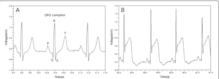
When a patient experiences coronary ischemic syndrome, his or her electrocardiogram (ECG) shows some peculiar appearances. Each segment of ECG can be divided into P, Q, R, S and T waves as shown in Figure 1 where QRS complex and T wave represent ventric-ular depolarization and repolarization, respectively. In most cases of normal ECG, the ST segment has the same electric potential as the PR segment. When myocardial ischemia is present, however, the electric potential of the ST segment is elevated or depressed with respect to the potential of the PR segment [1,2]. When ischemia occurs, the PR segment is altered, or the ST segment deviates from normal level. If the PR segment moved instead of the ST segment, this looks as if the ST segment itself were modified. This is because the PR segment provides a kind of reference voltage level [1].
The ST segment deviation is mainly due to injury current in myocardial cells [1]. If the coronary artery becomes blocked by blood clot, some myocytes are affected to be unresponsive to depolarization, or to repolarize earlier than adjacent myocytes. In this case, voltage gradient can occur in the myocytes, and this comes to appear as ST-segment deviation in ECG [1]. Figure 2 shows two cases when the voltage level of the ST segment deviates from its normal position. The left column of the figure shows the distribution of electric charges around myocytes when the heart is in resting state. This is related to the PR segment in ECG. The right column shows the distribution of electric charges right after the ventricles contracted. This is related to the QRS complex and the ST segment in ECG. The shaded region represents the area being affected by myocardial ischemia. In the case of the upper row in Figure 2, there is no voltage gradient at first. After the ventricles contracted, however, the voltage gradient comes to appear because the injured area did not respond to electric depolarization. In the second case of the bottom row, there is no voltage gradient right after the ventricles contracted. In the left figure, however, there was initial voltage gradient, and this makes the PR segment to be modified. The PR segment acts as a reference voltage level when we judge whether the ST segment deviated from normal position. The modified PR segment makes us conclude that there was a ST segment deviation [1].
Figure 2 Cause of ST segment deviation [1].Left column shows distribution of electric charges before the ventricles contracts. The right column shows the charge distribution after the ventricles contracted. Shaded area represents that the area was affected by ischemia.
of first 100 beats. They adopted an adaptive amplitude threshold to classify ECG sig-nal [14]. Murugan and Radhakrishnan used ant-miner algorithm to detect ischemic ECG beats. They calculated several feature values such as ST segment deviation from input ECG signal [15]. Bakhshipour et al. analyzed coefficients resulted from wavelet transform. They examined the relative quotient of the coefficients at each decomposition level of the wavelet transform [16].
We approached this problem by extracting feature values from a ECG waveform. We first found time positions of QRS complexes, and then determined values of the three features. We calculated the feature values for each heart beat, and averaged their values in five successive beats. After that, we classified them by the methods of kernel density estimation and support vector machine.
We showed techniques of removing baseline wandering and detecting time positions of QRS complexes by discrete wavelet transform. With these explicit methods of dealing with ECG, we could discriminate ischemic ST episode from normal ECG. We did not adopt implicit methods such as artificial neural networks or decision trees, because we considered it was important to utilize explicit features for processes of decision making. The artificial neural network has a kind of black box nature in its hidden layers [17], and a decision tree is apt to include several numerical thresholds [13].
Methods Materials
We used the European ST-T database from Physionet. European ST-T database has 90 records which are two-channel and each two hours in duration [18,19]. Each record in this database has a different number of ST episodes. Overall there are 367 ischemic ST episodes in the database. Sampling frequency of each ECG data is 250 Hz.
We excluded 5 records because these had some problems. The records e0133, e0155, e0509, and e0611 had no ischemic ST episodes. The record e0163 had so limited ST episode whose length was just 31 seconds.
Removing baseline wandering
The ST segments in ECG can be strongly affected by baseline wandering [20]. Main causes of the baseline wandering are respiration and electrode impedance change due to per-spiration [20,21]. The frequency content of the baseline wandering is usually in a range below 0.5 Hz [20,21].
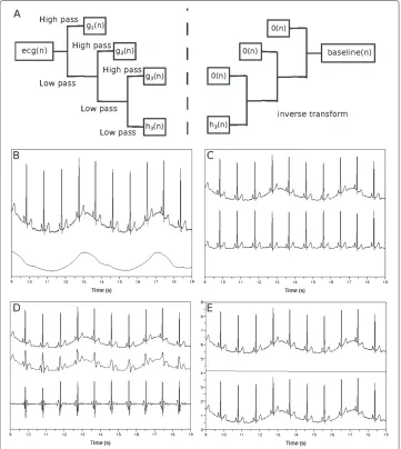
We use discrete wavelet transform to remove baseline wandering in ECG. We transform signal vector into two sequences of coefficients, approximation and detail coefficients sequences [22]. We do this in each step in an iterative fashion, until we get an input signal whose length is smaller than the length of the filter which characterizes the wavelet. In our case, we used Daubechies8 wavelet with filter length of 8. The resulting approximation coefficient sequence becomes the input signal to the next discrete wavelet transform as shown in Figure 3(a) [22].
Figure 3 Removing baseline wandering in ECG.(a) Discrete wavelet transform ofecg(n) to find coefficient sequenceshk(n),gk(n),gk−1(n),· · ·,g1(n). The0(n)means zero sequence. (b) Top: input ECG,ecg(n), bottom: wandering baseline in ECG,baseline(n). (c) Top:ecg(n), bottom:ecg(n)-baseline(n). Whenkis (d) too small or (e) too large, top:ecg(n), middle:baseline(n), bottom:ecg(n)-baseline(n).
ofg1(n)is from x4 to 2x, and the frequency content ofh1(n) is below x4. In this regard,
if we have transformed the ecg(n) into the approximation coefficient sequencehk(n), and the detail coefficient sequencesgk(n),gk−1(n),· · ·,g1(n), the frequency contents of
gk(n),gk−1(n),· · ·,g1(n)become
x
2k+1,2xk
,x
2k,2kx−1
,· · ·,2x2,x2respectively [24,25]. To remove baseline wandering, we should choose appropriate wavelet scale. We fol-low argument similar to that presented by Arvinti et al. except that they used stationary wavelet transform instead of its discrete counterpart [26]. We remove signal components whose frequency content is less than 1/2 Hz [20,21]. If we have transformed the ECG signal ecg(n) into coefficient sequences hk(n),gk(n),gk−1(n),· · ·,g1(n), the frequency
contents ofhk(n)andgk(n)become
0, x
2k+1
and x
2k+1,2xk
respectively, wherexis the
sampling frequency. If we choosekas x
2k+1 ≤ 12,k=
sequence0(n)to all the detail coefficient sequencesgk(n),gk−1(n),· · ·,g1(n), and
calcu-late inverse transform ofhk(n),0(n),0(n),· · ·,0(n)to form thebaseline(n) in the bottom of Figure 3(b). If we subtractbaseline(n) fromecg(n), we obtain the flattened signal like the one shown in Figure 3(c).
If we select a wrong wavelet scale k to find coefficient sequences of ecg(n), we obtain disappointing results. The flattened signal in Figure 3(c) is obtained when k is log2250 = 8, where 250 is the sampling frequency expressed in Hz. When select k=4 to use h4(n),g4(n),g3(n),g2(n),g1(n), we obtain a plot in Figure 3(d). The
middle waveform,baseline(n), resulted from the inverse discrete wavelet transform of h4(n),0(n),0(n),0(n)0(n). This middle waveform is too detailed, so the bottom
wave-formecg(n)-baseline(n) was negatively affected. When we selectk=12, see Figure 3(e), the bottom waveform was not different from the input waveformecg(n).
We adopt a discrete wavelet transform to retain the details of the ECG waveform because filtering by some cut-off frequency can deteriorate the quality of the ECG waveforms [27].
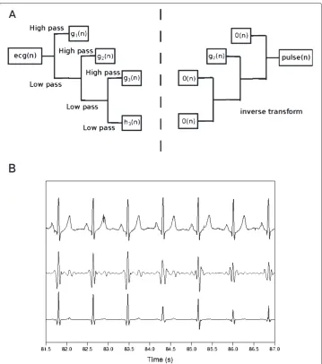
Detecting QRS complexes
We have to select an appropriate wavelet scale to capture proper time positions of QRS complexes. We will deal with only the flattened ECG waveformecg(n)-baseline(n) referred in the previous section. We will denote it asfecg(n).
First, we determine the sequences of wavelet coefficients of the fecg(n), obtain-ing hk(n),gk(n),gk−1(n),· · ·,g1(n) where k =
log2x, x is sampling frequency. We assign zero to all the coefficient sequences except one, gj(n). Then, we calculate inverse transform of0(n)(approximation coefficients),0(n)(detail coefficients, onward), · · ·,0(n),gj(n),0(n),· · ·,0(n)to obtainpulse(n). To find a protruding segment, that is, a QRS complex, we compute the score for each wavelet scalej,
scorej=
l
fecg(l)pulse(l)
mpulse(m)
.
We select the wavelet scalejwhich produces the largest drop ofscorej−scorej+1(j≥2).
The bottom waveform in Figure 4(b) shows the time positions of QRS complexes when selecting this suitable wavelet scale.
After finding the locations of QRS complexes, we choose QRS onset and offset points in each QRS complex. We search QRS onset point in backward direction from a peak point in each QRS complex. We take the QRS onset point if the point is at the place of changing direction of rising and falling offecg(n) twice. In the same way, we take the QRS offset point in forward direction from the peak point.
Algorithm 1 shows a process of removing baseline wandering and detecting QRS complexes.
Algorithm 1 A procedure to find time positions of QRS onset, peak and offset points. This procedure includes the method of removing baseline wandering in ECG. nBeats stands for the number of QRS peaks. It is the length of the sequences idx_QRS_Onset(n), idx_QRS_Peak(n) and idx_QRS_Offset(n).
Input:Sampling_Hz,ecg(n)
Output:idx_QRS_Onset(n), idx_QRS_Peak(n), idx_QRS_Offset(n)
k←log2Sampling_Hz
Discrete wavelet transform (DWT) ofecg(n)intohk(n),gk(n),gk−1(n),· · ·,g1(n)
fori=1 tokdo
gi(n)← 0(n){//0(n)means zero sequence.}
end for
Inverse wavelet transform (IDWT) ofhk(n),gk(n),gk−1(n),· · ·,g1(n)into
baseline(n)
fecg(n)←ecg(n)−baseline(n)
DWT offecg(n)intohk(n),gk(n),gk−1(n),· · ·,g1(n)
gk(n)← 0(n) fori=1 tok−1do
gi(n)←gi(n) gi(n)← 0(n) end for
fori=1 tok−1do gi(n)←gi(n)
IDWT ofhk(n),gk(n),gk−1(n),· · ·,g1(n)intopulse(n)
scorei←lfecg(l)|pulse(l)| m|pulse(m)|
gi(n)← 0(n) end for
chosen_scale←argmax2≤i≤k−2{scorei−scorei+1}
gchosen_scale(n)←gchosen_scale (n)
IDWT ofhk(n),gk(n),gk−1(n),· · ·,g1(n)intopulse(n)
needle(n)←fecg(n)pulse(n)
Make idx_QRS_Peak(n)by searching for local maxima ofneedle(n)
fori=1 tonBeatsdo
iffecg(idx_QRS_Peak(i)) >0then j←1
whilefecgidx_QRS_Peak(i)−j≤fecgidx_QRS_Peak(i)−j+1do j←j+1
end while
whilefecgidx_QRS_Peak(i)−j>fecgidx_QRS_Peak(i)−j+1do j←j+1
end while
idx_QRS_Onset(i)←idx_QRS_Peak(i)−j j←1
whilefecgidx_QRS_Peak(i)+j−1≥fecgidx_QRS_Peak(i)+jdo j←j+1
end while
whilefecgidx_QRS_Peak(i)+j−1<fecgidx_QRS_Peak(i)+jdo j←j+1
end while
idx_QRS_Offset(i)←idx_QRS_Peak(i)+j else
· · ·{//When QRS complex protrudes downward, code is same with reversing directions of inequality signs.}
end if end for
Feature formation for classification problems
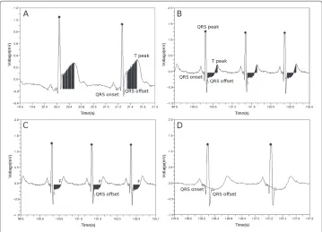
To form the first feature, we sum up all the voltage deviation from QRS offset point to T wave peak point as shown in Figure 5(a) and (b).
feature1=
Tpeak
i=QRSoffset
fecg(i)−fecg(QRSonset)
The second feature is similar to the first feature with an exception of the ending position of the sum. We terminate the summation as we reach the first point, F, at which the voltage becomes equal to the reference voltagefecg(QRSonset), see Figure 5. When doing this, we add the signed values of the voltage deviation to find whether the area is lower or higher with respect to the reference voltage. Then we divide the value by the voltage at QRS peak point. The second feature value is given as follows.
feature2= ⎛
⎝ F
i=QRSoffset
fecg(i)−fecg(QRSonset) ⎞
⎠/fecg(QRSpeak)
The third feature is a slope from the QRS onset point to the QRS offset point.
feature3=
fecg(QRSQRSoffsetoffset)−−fecgQRS(onsetQRSonset)
We calculate these three feature values for each heart beat. Then we average these values in five successive beats, and arrange the three mean values asfeature1,feature2,feature3
.
Algorithm 2 shows the pseudo-code of computing feature values.
Algorithm 2 A procedure to compute feature values. nBeats denotes the number of QRS peaks. It is the length of the sequences idx_QRS_Onset(n), idx_QRS_Peak(n)and idx_QRS_Offset(n).nclis equal tonBeats/5.
Input:fecg(n), idx_QRS_Onset(n), idx_QRS_Peak(n), idx_QRS_Offset(n)
Output:
x(1cl),x2(cl),· · ·,x(nclcl)
{//clcan beS(ST episode) orN(normal).}
mean_idx_diff1←
nBeats
i=1 (idx_QRS_Peak(i)−idx_QRS_Onset(i))
/nBeats
mean_idx_diff2←nBeatsi=1 (idx_QRS_Offset(i)−idx_QRS_Peak(i))
/nBeats {//mean_idx_diff1and mean_idx_diff2are truncated into integers.}
fecg(QRSonset)←inBeats=1 fecg(idx_QRS_Onset(i))
/nBeats fori=1 tonBeatsdo
k←idx_QRS_Peak(i)+mean_idx_diff2
feature1(i)←Tj=peakk fecg(j)−fecg(QRSonset)
feature2(i)←Fj=k
fecg(j)−fecg(QRSonset)
/fecg(idx_QRS_Peak(i)) m←idx_QRS_Peak(i)−mean_idx_diff1
feature3(i)←fecg(kk)−−fecgm (m)
end for
fori=1 tonBeats/5
x(icl)
1←
1 5
5i
j=5i−4feature1(j)
x(icl)
2←
1 5
5i
j=5i−4feature2(j)
x(icl)
3←
1 5
5i
j=5i−4feature3(j)
end for
Classification by kernel density estimation
We approximate probability density at a point by considering the other points. Let us assume we haved-dimensional points{x1,x2,· · ·,xn}. We can estimate the probability density at a pointyasp(y)= n1KV whereVis a small volume aroundy, andKis a num-ber of enclosed points in the volumeV [29]. We replace the term KV by d-dimensional Gaussian function as follows [30].
p(y)= 1
n K V = 1 n n
i=1
1 √
2πd1/2
e−12(y−xi)T
−1
(y−xi)
If we assume that the covariance matrix is a diagonal matrix with each diagonal elementb2j 1≤j≤d, the probability density at the pointyis given as follows [31].
p(y)= 1
n n
i=1
1 √
2πd(b1b2· · ·bd) e− 1 2 d j=1 [y]j−[xi]j
bj 2
We classify a test point by examining posterior probabilities in which the test point belongs to two classes, normal or ischemic ST episode. We assume we havenS points
x(1S),x2(S),· · ·,x(nSS)
, andnN points
x(1N),x2(N),· · ·,x(nNN)
. The first and the second set designate training sets of ischemic ST episode and normal part, respectively. Each point is described by three componentsfeature1,feature2,feature3
We compute posterior probability in which the test pointybelongs to each class by Bayes’ theorem as follows [29].
P(class|y)= P(class)p(y|class)
P(class=N)p(y|class=N)+P(class=S)p(y|class=S)
The prior probability P(class) is given as P(class=N) = nN/ (nN+nS) or P(class=S)=nS/ (nN+nS). The likelihoodp(y|class=N)andp(y|class=S)reads as
p(y|class=N)= 1
nN
√ 2π3
b(1N)b(2N)b(3N)
nN
i=1
e −1 2 3 j=1 ⎛ ⎝[y]j−
x(iN)
j
bj(N) ⎞ ⎠
2
,
p(y|class=S)= 1
nS
√ 2π3
b(1S)b(2S)b(3S) nS
i=1
e −1 2 3 j=1 ⎛ ⎝[y]j−
x(iS)
j
b(jS) ⎞ ⎠
2
.
The quantities b(iN) and bi(S) (1≤i≤3) are called kernel bandwidths. We calculate these bandwidths for each class (N or S) and component (1≤i≤3). These kernel bandwidths impact accuracy of kernel density estimation [32].
We havencl training points
x(1cl),x2(cl),· · ·,x(nclcl)
wherecldenotes class,N (normal) or S (ischemic ST episode). For each component(1≤i≤3) of the feature vector, we calculate the mean value of differences as follows.
mean(icl)= 1 ncl(ncl−1) /2
ncl
j=1
ncl
k=j+1 x(jcl)
i−
x(kcl)
i
We choose half of the mean,12mean(icl), as kernel bandwidthb(icl)for each classcl(Nor S), and componenti(1≤i≤3).
Classification with the use of support vector machine
Let us assume we havencltraining points
x(1cl),x2(cl),· · ·,x(nclcl)
. Each point is described as
feature1,feature2,feature3
in a three-dimensional feature space. We construct support vector machine classifier by solving the following optimization problem [33]
min
w,b,ξ
⎧ ⎨ ⎩ 1 2w
T·w+C ncl
j=1 ξj
⎫ ⎬ ⎭
subject to t(icl)
wT·φ
x(icl)
+b
≥1−ξi, ξi≥0.
The target labelt(icl)is specified as 1 (normal) or -1 (ischemic ST episode). The parameter Ccontrols the trade-off between the slack variable (ξi) penalty and the margin (wT ·w) penalties [29]. The dual form of the above classifier reads as follows
max α ⎧ ⎨ ⎩ ncl
j=1 αj−
1 2α
T ·Hα
⎫ ⎬ ⎭
subject to
ncl
j=1
where the matrix H is expressed as Hij ≡ ti(cl)t(jcl)K
x(icl),x(jcl)
= ti(cl)t(jcl)φ
x(icl)
·
φ
x(jcl)
= t(icl)t(jcl)e− 1 3x
(cl) i −x
(cl) j
2
[33]. When we classify a new pattern y, we
exam-ine decision function, sgnncl
j=1t (cl)
j αjK
x(jcl),y
+b. Whenever the input training set
x(1cl),x2(cl),· · ·,x(nclcl)
was changed, we varied the parameter C to find its value which produced the highest classification rate.
Experiments setting
We used kernel density estimation and support vector machine methods to evaluate the proposed approach. We completed the experiment for each channel and record available in the European ST-T database. First, we trained the classifier based on a subset of ST episodes and normal ECG. Then we tested how well the feature values discriminated the two classes, ST episode and normal. When we formed the ST episode data, we used all the ischemic ST episodes except ST deviations data resulted from non-ischemic causes such as position related changes in the electrical axis of the heart. To preserve balance between ST episode and normal ECG data, we collected normal data from the beginning of each record as much as the amount of ST episode data. When dividing the data into training and test sets, we assigned one tenth of data to the training data, and the rest to the test data. In the cases of e0106 lead 0, e0110, e0136, e0170, e0304, e0601, and e0615 records, we constructed the training data of one third of all data and test data of two thirds because these records had much small ischemic ST episode data. To avoid ambiguous region between ischemic ST episode and normal ECG, we removed 10 seconds amount of ECG data from each side of the boundary.
When we classified a test setyi
, four quantities were computed: true positive (TP), false negative (FN), false positive (FP), and true negative (TN). TP is a number of ischemic events correctly detected. FN is a number of erroneously rejected (missed) ischemic events. FP is a number of non-ischemic, that is, normal parts which the clas-sifier erroneously detected as ischemic events. TN is a number of normal parts which our classifier correctly rejected as non-ischemic events [34]. These are numbers of cor-respondingyipoints which were obtained by averaging three feature values of successive five beats in Algorithm 2. The sensitivity and specificity are expressed in a usual fashion, Se=TP/(TP+FN)andSp=TN/(TN+FP)respectively [6].
We tested the classifiers by counting how many ST episodes were correctly caught, out of 367 episodes in the 85 records of European ST-T database. For an interval of ischemic ST episode data, we formedntest pointsy1,y2,· · ·,yn
from the data (Algorithm 2), and classified each test point and then counted numbers of two classes, “ischemic” and “nor-mal”. If the number of class “ischemic” was larger thann/2, we declared the interval to be an ischemic ST episode. The experiments were completed for 367 ischemic ST episodes. We compared the results of kernel density estimation (KDE) and support vector machine (SVM) methods with those formed by artificial neural network (ANN). The corresponding ANN classifier exhibits the following topology. The input layer has three nodes which acceptfeature1,feature2andfeature3respectively. The output layer has two
backpropagation method [17] for 3000 iterations. We used a sigmoid activation function 1/1+e−xand set learning rate 0.01. We adopted various topologies of hidden layers such as 3 → (5) → (5) → 2, 3 → (6) → 2, 3 → (7) → 2 and 3 → (8) → 2 where the number in each parenthesis represents a number of nodes in the corresponding hid-den layer. We used stochastic (incremental) gradient descent method to alleviate some drawbacks of the standard gradient descent method, see [17].
Results
KDE with various kernels
We can use various kernels in kernel density estimation. If we have training points {x1,x2,· · ·,xn}and a test pointy, the probability density atyis given as follows [35].
p(y)= 1
n n
i=1
kG b1b2b3
e−12u2i (Gaussian),
p(y)= 1
n n
i=1
kR b1b2b3
1{|ui|≤1} (Rectangular),
p(y)= 1
n n
i=1
kE b1b2b3
1−u2i1{|ui|≤1} (Bartlett-Epanechnikov),
p(y)= 1
n n
i=1
kB b1b2b3
1−u2i21{|ui|≤1} (Byweight),
p(y)= 1
n n
i=1
kTriw b1b2b3
1−u2i31{|ui|≤1} (Triweight),
p(y)= 1
n n
i=1
kTria b1b2b3
(1−ui)1{|ui|≤1} (Triangular).
Here kG, kR, kE, kB, kTriw and kTria are constants, and u2i is given as u2i ≡
3
j=1
[y]j−[xi]j
bj 2
because we use three feature values. The indicator function1{|ui|≤1}is
given as follows.
1{|ui|≤1}=
1 (if |ui| ≤1) 0 (otherwise)
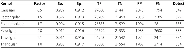
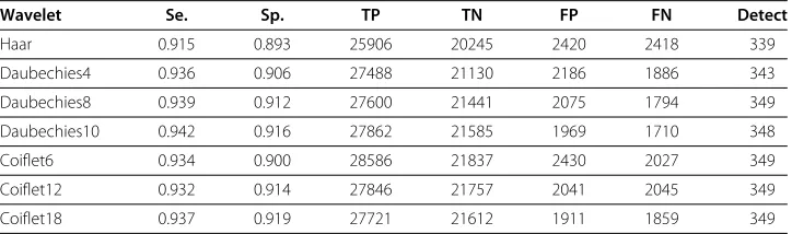
Table 1 shows classification results for various kernels. In all cases we used Daubechies8 wavelet to produce training and test sets. We took each bandwidthb(icl) = mean(icl) · factorfor classcl, ischemic or normal, and 1≤i≤3. The “detect” means how many ST
Table 1 Classification results with respect to various kernels
Kernel Factor Se. Sp. TP TN FP FN Detect
Gaussian 0.5 0.939 0.912 27600 21441 2075 1794 349
Rectangular 1.5 0.892 0.913 26209 21460 2056 3185 329
Epanechnikov 1.7 0.904 0.915 26583 21522 1994 2811 335
Byweight 2.0 0.912 0.916 26794 21533 1983 2600 333
Triweight 2.1 0.916 0.916 26923 21542 1974 2471 336
Table 2 Classification results of Gaussian kernels with respect to various bandwidths
Factor Se. Sp. TP TN FP FN Detect
0.2 0.943 0.867 27728 20399 3117 1666 353
0.3 0.944 0.893 27745 20996 2520 1649 352
0.4 0.942 0.905 27697 21279 2237 1697 351
0.5 0.939 0.912 27600 21441 2075 1794 349
0.6 0.934 0.915 27453 21526 1990 1941 343
0.7 0.929 0.916 27318 21550 1966 2076 338
0.8 0.924 0.916 27148 21529 1987 2246 337
episodes our classifier correctly detected, out of total 367 episodes. The “factor” in this table specifies how we multiplied on themean(icl)to form the kernel bandwidthb(icl). We varied this factor from 0.1 to 3.0, and selected the one for which a sum of sensitivity and specificity values attains a maximum. Because the Gaussian kernel produced best results, in the sequel we will use the Gaussian kernel. Table 2 shows the results with respect to various kernel bandwidths.
Results for KDE, SVM and ANN with various wavelets
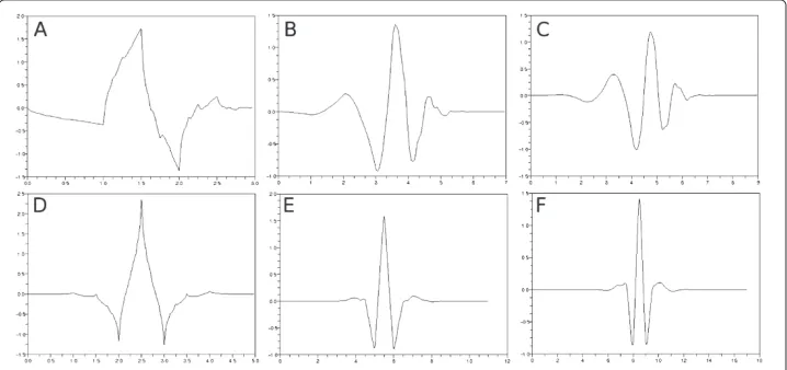
We examined the classifiers to find out how their performance depends on the mother wavelets which were used to produce training and test sets in Algorithm 1. We used 7 wavelets, Haar, Daubechies4, Daubechies8, Daubechies10, Coiflet6, Coiflet12 and Coiflet18 [22,36]. The number forming a part of the name of each wavelet designates the length of filter which characterizes corresponding wavelet. Figure 6 shows selected shapes of wavelet functions except for the Haar wavelet which is given as
Haar(t)= 1 (0≤t≤1/2) −1 (1/2≤t≤1) .
Table 3 shows the classification results obtained for KDE. The kernel bandwidth is expressed asb(icl)=meani(cl)/2 for each classcland 1≤i≤3. We used Gaussian kernel.
Table 3 Classification results for KDE with respect to various wavelets
Wavelet Se. Sp. TP TN FP FN Detect
Haar 0.915 0.893 25906 20245 2420 2418 339
Daubechies4 0.936 0.906 27488 21130 2186 1886 343
Daubechies8 0.939 0.912 27600 21441 2075 1794 349
Daubechies10 0.942 0.916 27862 21585 1969 1710 348
Coiflet6 0.934 0.900 28586 21837 2430 2027 349
Coiflet12 0.932 0.914 27846 21757 2041 2045 349
Coiflet18 0.937 0.919 27721 21612 1911 1859 349
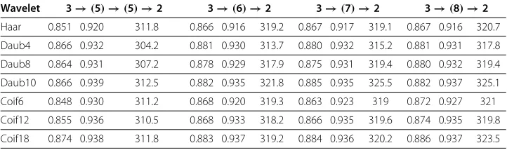
Table 4 shows the classification results for the KDE with respect to various bandwidths and wavelets. The first column for each wavelet item represents the sum of sensitivity and specificity. The second column shows how many ST episodes were correctly detected. We used the kernel bandwidthsb(icl)= meani(cl)·factorfor each classcland 1≤i≤3. The sum of sensitivity and specificity becomes maximum when the bandwidthb(icl)is around b(icl)≈mean(icl)/2.
Table 5 shows the classification results obtained for SVM. The parameterCcontrols the trade-off between the slack variable (ξi) penalty and the margin (wT·w) penalties. We examined the classification accuracy versus the values ofCchanging from 0.1 to 300.0 in step of 0.1, and selected the one that made the sum of sensitivity and specificity maximal. Table 6 shows the classification results obtained by ANN. The number in parenthe-sis represents the number of nodes in the corresponding hidden layer. The first, second and third column express sensitivity, specificity and the “detect” respectively. We experi-mented 10 times, and averaged the results because we obtained different results each time due to the random initialization of weights.
Table 4 Classification results for KDE versus selected values of bandwidths and types of wavelets
Factor Haar Daub4 Daub8 Daub10 Coif6 Coif12 Coif18
0.2 1.770 348 1.797 348 1.811 353 1.817 355 1.794 356 1.812 360 1.825 354
0.3 1.797 350 1.825 350 1.837 352 1.843 356 1.822 354 1.833 357 1.848 353
0.4 1.808 345 1.838 344 1.847 351 1.856 353 1.833 354 1.844 355 1.857 354
0.5 1.808 339 1.842 343 1.851 349 1.859 348 1.834 349 1.846 349 1.856 349
0.6 1.806 336 1.840 339 1.849 343 1.857 343 1.832 345 1.843 346 1.854 346
0.7 1.800 331 1.836 336 1.846 338 1.853 338 1.829 340 1.837 341 1.849 344
0.8 1.792 325 1.829 334 1.839 337 1.848 335 1.824 334 1.831 339 1.842 340
Table 5 Classification results for SVM for various wavelets
Wavelet C Se. Sp. TP TN FP FN Detect
Haar 291.3 0.924 0.907 26163 20547 2118 2161 345
Daubechies4 242.9 0.937 0.923 27527 21519 1797 1847 349
Daubechies8 245.5 0.941 0.923 27658 21712 1804 1736 355
Daubechies10 174.3 0.943 0.927 27894 21838 1716 1678 349
Coiflet6 288.2 0.933 0.918 28571 22284 1983 2042 348
Coiflet12 52.8 0.929 0.918 27757 21858 1940 2134 348
Table 6 Results for ANN classifiers with respect to various wavelets and sizes of hidden layers
Wavelet 3→(5)→(5)→2 3→(6)→2 3→(7)→2 3→(8)→2
Haar 0.851 0.920 311.8 0.866 0.916 319.2 0.867 0.917 319.1 0.867 0.916 320.7
Daub4 0.866 0.932 304.2 0.881 0.930 313.7 0.880 0.932 315.2 0.881 0.931 317.8
Daub8 0.864 0.931 307.2 0.878 0.929 317.9 0.875 0.931 319.4 0.880 0.932 319.4
Daub10 0.866 0.939 312.5 0.882 0.935 321.8 0.885 0.935 325.5 0.882 0.937 325.1
Coif6 0.848 0.930 311.2 0.868 0.920 319.3 0.863 0.923 319 0.872 0.927 321
Coif12 0.855 0.936 310.5 0.868 0.933 318.2 0.866 0.935 319.6 0.874 0.935 319.8
Coif18 0.874 0.938 311.8 0.883 0.937 319.2 0.884 0.936 320.2 0.886 0.937 323.5
Tables 3, 5 and 6 show that the Daubechies8 and Daubechies10 wavelets give us superior results. The shapes of these two wavelets are similar to typical ECG waveforms [37,38]. From now on, we use the Daubechies8 wavelet exclusively.
Effects of baseline wandering in ECG
Table 7 shows the classification results by KDE, SVM and ANN when we did not remove baseline wandering in ECG. If we compare this table with the Tables 3, 5 and 6, we get to know it is essential to remove baseline wandering in Algorithm 1. In the Table 7, we selected the kernel bandwidths b(icl) in the KDE classifier as bi(cl) = mean(icl)/2, (1≤i≤3). We used the ANN classifier with sizes of layers expressed as 3→(7) →2. The results of ANN were obtained by averaging results for 10 repetition of the experiments. The parameterCof the SVM classifier was 297.9.
If we use unsuitable wavelet scale like the one in Figure 3 to remove baseline wandering, it becomes difficult to obtain good results. As the sampling frequency was 250 Hz, we selected the wavelet scalelog2250=8 in Algorithm 1. Table 8 shows the classification results when wrong wavelet scales were selected. The kernel bandwidth setting in KDE and layer composition of ANN classifier were same as the Table 7. The middle row of wavelet scale 8 in Table 8 was our choice in Algorithm 1. Each entry in the row of wavelet scale 8 has counterparts in “Daubechies8” rows in Tables 3, 5 and 6.
Table 7 Classification results for KDE, SVM and ANN without removal of baseline wandering
Se. Sp. TP TN FP FN Detect
KDE 0.852 0.837 22132 17211 3342 3839 328
SVM 0.870 0.835 22605 17161 3392 3366 326
ANN 0.785 0.827 20388.8 17005.7 3547.3 5582.2 296.1
Table 8 Classification results for KDE, SVM and ANN with incorrectly selected wavelet scales to remove baseline wandering
KDE SVM ANN
Se. Sp. Detect Trade-off Se. Sp. Detect Se. Sp. Detect
scale 6 0.851 0.785 319 288.2 0.842 0.818 318 0.748 0.864 277.5
scale 7 0.931 0.905 344 232.8 0.932 0.915 349 0.876 0.933 320.7
scale 8 0.939 0.912 349 245.5 0.941 0.923 355 0.875 0.931 319.4
scale 9 0.929 0.906 347 110.4 0.930 0.918 350 0.859 0.918 320.7
Figure 7 ECG signal affected by synthetic noise.(a) Original signal. (b) Noise-affected signal whenais 1.0 andbis 6.0.
Effects of simulated noise
We examined performance of the classifiers when we added simulated noise into the orig-inal ECG signal. We modeled the noise as the sum of wandering baseline and AC power line 60 Hz noise.
Let us assume we have original signal data, ecg(i) (1≤i≤n). First, we compute mean value and standard deviation of the ECG signal as m = ni=1ecg(i)/n and
s=!ni=1ecg(i)2
/n−m2. Then we form a new signalecg(i)by
ecg(i)=ecg(i)+s·a·
sin
b· i Samp_Freq
+ 1
2cos
2π60· i Samp_Freq
whereais an amplification factor andbis an angular frequency of the added baseline. HereSamp_Freqmeans sampling frequency which was 250 Hz in our case. We varieda from 0.1 to 1.0 in step of 0.1, and selectedbto be equal to 2, 4 or 6.
Figure 7 shows the original ECG and its noise-impacted version. Tables 9, 10 and 11 show the experimental results for the noisy ECG signal. The first, second and third col-umn in eachbitem represent the sensitivity, specificity and the “detect” respectively. The kernel bandwidth is set asb(icl) = mean(icl)/2 for the KDE classifier. The layer composi-tion of the ANN classifier was 3→(7)→2. The first column in eachbitem in Table 10 includes the trade-off parameterCwhich produced best results.
Table 9 Classification results for KDE versus varying intensity of noise
a b=2 b=4 b=6
0.1 0.937 0.903 346 0.934 0.902 346 0.933 0.904 346
0.2 0.933 0.893 346 0.927 0.892 341 0.916 0.879 337
0.3 0.929 0.884 342 0.915 0.873 340 0.908 0.856 338
0.4 0.925 0.864 346 0.903 0.852 344 0.885 0.834 327
0.5 0.916 0.858 346 0.882 0.848 333 0.871 0.817 333
0.6 0.906 0.866 343 0.872 0.832 329 0.858 0.803 321
0.7 0.891 0.856 340 0.859 0.815 325 0.848 0.794 322
0.8 0.887 0.850 339 0.852 0.799 325 0.838 0.793 317
0.9 0.881 0.849 341 0.837 0.798 312 0.837 0.778 301
Table 10 Classification results for SVM with varying intensity of the simulated noise
a b=2 b=4 b=6
0.1 79.0 0.936 0.920 350 254.6 0.940 0.915 352 147.4 0.936 0.916 349
0.2 143.0 0.929 0.914 347 168.5 0.929 0.904 349 33.9 0.922 0.888 339
0.3 84.1 0.923 0.910 348 50.9 0.915 0.891 341 72.3 0.902 0.875 337
0.4 124.5 0.919 0.899 348 51.3 0.903 0.869 341 52.0 0.888 0.848 330
0.5 65.1 0.909 0.895 347 86.7 0.882 0.859 333 79.4 0.872 0.828 328
0.6 96.7 0.903 0.887 343 67.3 0.879 0.844 330 71.6 0.865 0.809 323
0.7 119.3 0.888 0.880 339 27.2 0.868 0.832 329 36.6 0.856 0.796 313
0.8 201.8 0.893 0.863 334 24.9 0.851 0.829 320 27.1 0.848 0.785 310
0.9 278.2 0.888 0.857 335 16.7 0.841 0.816 308 71.0 0.850 0.777 315
1.0 211.7 0.879 0.859 324 58.2 0.835 0.806 311 20.3 0.837 0.776 317
Comparison with others’ works
To compare our approach with others’ works, we tested the classifiers on 10 selected records, e0103, e0104, e0105, e0108, e0113, e0114, e0147, e0159, e0162 and e0206. Table 12 shows results of comparison. The papers by Papaloukas et al. [10], Goletsis et al. [39], Exarchos et al. [13] and Murugan et al. [15] in Table 12 dealt with the 10 records.
We used the Daubechies8 wavelet in Algorithm 1 to analyze the ECG waveform, and took the kernel bandwidthsb(icl)=mean(icl)/2 for the KDE classifier with Gaussian kernel. We used the SVM classifier withC=281.1.
Discussion
Table 1 showed how the classification results were dependent on various kernel functions in kernel density estimation. Gaussian kernel produced best results.
Tables 3, 4, 5 and 6 show how the classification results depend on mother wavelets used in Algorithm 1. Daubechies8 and Daubechies10 wavelets were best. Because we imple-mented wavelet transform program with the use of matrix multiplication, we selected Daubechies8 wavelet to reduce computational burden. Daubechies10 wavelet did not produce much better classification accuracy than Daubechies8 wavelet.
Tables 2 and 4 indicate that the choice of kernel bandwidths was reasonable. When we took the kernel bandwidthsb(icl) = meani(cl)/2 for classcl, 1 ≤ i ≤ 3, we obtained best results except for the case of Coiflet18 wavelet. Even in the case, the best parameter
Table 11 Classification results for ANN with varying intensity of the simulated noise
a b=2 b=4 b=6
0.1 0.880 0.929 322.2 0.870 0.921 320.8 0.874 0.922 320.3
0.2 0.867 0.928 322.8 0.844 0.922 315.1 0.840 0.905 314.2
0.3 0.863 0.929 319.3 0.837 0.906 313.4 0.811 0.895 303.4
0.4 0.856 0.917 320.5 0.823 0.887 312.3 0.784 0.874 300.6
0.5 0.830 0.918 320.1 0.811 0.874 309.1 0.778 0.850 300.3
0.6 0.818 0.916 314.9 0.803 0.858 299.2 0.762 0.833 292
0.7 0.803 0.910 309.6 0.759 0.865 281.9 0.761 0.811 283.2
0.8 0.814 0.898 308.6 0.753 0.839 288.2 0.745 0.801 280.7
0.9 0.798 0.892 303.4 0.723 0.838 273.9 0.728 0.795 261.7
Table 12 Results of comparative analysis
Researcher Sensitivity Specificity
Papaloukas et al. [10] 0.90 0.90
Goletsis et al. [39] 0.912 0.909
Exarchos et al. [13] 0.912 0.922
Murugan et al. [15] 0.923 0.943
Present work by KDE 0.945 0.943
Present work by SVM 0.957 0.953
b(icl) = 0.4·mean(icl)was close enough tob(icl) = mean(icl)/2. We maintained this choice in Tables 7, 8 and 9. In this way, we could automatically select 6 kernel bandwidths, and this exempted us from choosing any numerical parameters.
The SVM classifiers in Tables 5, 7 and 8 produced better results than the KDE classifiers, but they required us to determine optimal value of the parameterC. Whenever we used different wavelets on the same data set in Table 5, we had to choose different trade-off parameterC. This was also the case in Table 8 where we intentionally selected incorrect wavelet scales to remove baseline wandering.
Order of magnitude offeature3was very different fromfeature1andfeature2. When
we produced the feature values using Daubechies8 wavelet in Algorithm 1, mean val-ues offeature1,feature2andfeature3were 7.327, 7.613 and 0.004, respectively. Thus
we had to normalize the feature values to use them in classification. Even if the orders of magnitude offeature1,feature2andfeature3were very different, the equation of
ker-nel density estimation included a term 1 b(1cl)b(2cl)b(3cl)
ie
−1 2
3 j=1
⎛ ⎜ ⎝
[y]j−
#
x(icl)
$
j
b(jcl) ⎞ ⎟ ⎠
2
. Furthermore
each operand in the sum comes in the form of [
y]j−
x(icl)
j
b(jcl)
, normalization by kernel
bandwidth. We thought these would be helpful to overcome the difference of order of magnitude betweenfeature1,feature2andfeature3. This was a main driving force to adopt
the kernel density estimation.
We implemented the KDE and ANN classifier in C language for ourselves. For SVM classifier, we used libsvm library [33]. We compiled the programs with gcc and g++ with-out using any SIMD (single instruction multiple data) math library. Total amount of ECG text files which we used in our analysis was 200.4 MB. This amount is just about volt-age information not including time information. When we ran our programs to process the ECG text files in Pentium4 3.2 GHz CPU, it took 243.0 seconds until the procedures of removing baseline wandering and detecting time positions in Algorithm 1 were com-pleted. This was when we used Daubechies8 wavelet. Feature extraction in Algorithm 2, required 0.6 seconds. It took 1.2 seconds for the KDE classifier to process all the files. The SVM classifier required 0.8 seconds for the same job. The ANN classifier with layer composition 3→(7)→2 required 94.7 seconds.
59.5 seconds which was approximately four times faster than ours. However the KDE classifier produced the results ofsensitivity, specificity, detectbeing (0.904, 0.891, 329). These results are somewhat inferior compared to the results in Table 2.
Conclusions
The ST segment deviation in ECG can be an indicator of myocardial ischemia. If we can predict an ischemic syndrome as early as possible, we will be able to prevent more severe heart disease such as myocardial infarction [8,9].
To detect ischemic ST episode, we adopted a method directly using morphological fea-tures of ECG waveforms. We did not use weight tuning methods such as artificial neural network or decision tree because we wanted to show explicitly which features of ECG waveforms were meaningful to detect ischemic ST episodes. In this regard, we calculated three feature values for each heart beat. They were area between QRS offset and T-peak points, normalized and signed sum from QRS offset to effective zero voltage point, and slope from QRS onset to offset point. After calculating these feature values for each heart beat, we averaged the values of successive five beats because we wanted to reduce out-lier effects. The order of magnitude of the third feature value, the slope from QRS onset to offset point, was very different from the other two feature values. To take care of this problem, we considered classification method by kernel density estimation.
We described how we removed baseline wandering in ECG, and detected time posi-tions of QRS complexes by the discrete wavelet transform. Since our classifier selects automatically kernel bandwidths in kernel density estimation, virtually it does not require any numerical parameter which operator should provide. In the tests, SVM with opti-mal parameters showed just a slightly better classification accuracy than the proposed method, but finding those parameters is a heavy burden compared with the proposed method. We can conclude that overall our proposed method is efficient enough and has more advantages than existing methods.
Competing interests
The authors declare that they have no competing interests.
Acknowledgements
This work was supported by the systems biology infrastructure establishment grant provided by Gwangju Institute of Science & Technology, Korea.
Author details
1School of Information and Communications, Gwangju Institute of Science and Technology 1, Oryong-dong, Buk-gu, Gwangju, Republic of Korea.2Department of Electrical and Computer Engineering, University of Alberta, Canada and Systems Research Institute, Polish Academy of Sciences, Warsaw, Poland.
Authors’ contributions
Mr. Park implemented the whole algorithm, and wrote the manuscript. Dr. Pedrycz proofread it and provided useful technical comments. Dr. Jeon designed the experiments and checked the validity of the proposed methods. All authors read and approved the final manuscript.
Received: 21 January 2012 Accepted: 23 May 2012 Published: 15 June 2012
References
1. Kusumoto FM:Cardiovascular Pathophysiology. North Carolina: Hayes Barton Press; 2004.
2. Brownfield J, Herbert M:EKG Criteria for Fibrinolysis: What’s Up with the J Point?Western Journal of Emergency Medicine2008,9:40–42.
3. Rabbani H, Mahjoob MP, Farahabadi E, Farahabadi A, Dehnavi AM:Ischemia detection by electrocardiogram in wavelet domain using entropy measure.Journal of Research in Medical Sciences2011,16(11):1473–1482. 4. Lemire D, Pharand C, Rajaonah J, Dube B, LeBlanc AR:Wavelet time entropy, T wave morphology and
5. Pang L, Tchoudovski I, Braecklein M, Egorouchkina K, Kellermann W, Bolz A:Real time heart ischemia detection in the smart home care system.InProceedings IEEE Engineering Medicine Biology Society; 2005:3703–3706.
6. Tonekabonipour H, Emam A, Teshnelab M, Shoorehdeli MA:Ischemia prediction via ECG using MLP and RBF predictors with ANFIS classifiers.InSeventh International Conference on Natural Computation; 2011:776–780. 7. Stamkopoulos T, Diamantaras K, Maglaveras N, Strintzis M:ECG analysis using nonlinear PCA neural networks
for ischemia detection.IEEE Transactions on Signal Processing1998,46(11):3058–3067.
8. Maglaveras N, Stamkopoulos T, Pappas C, Strintzis MG:An adaptive backpropagation neural network for real-time ischemia episodes detection: development and performance analysis using the European ST-T database.IEEE transactions on bio-medical engineering1998,45:805–813.
9. Afsar FA, Arif M, Yang J:Detection of ST segment deviation episodes in ECG using KLT with an ensemble neural classifier.Physiological measurement2008,29(7):747–760.
10. Papaloukas C, Fotiadis DI, Likas A, Michalis LK:An ischemia detection method based on artificial neural networks.Artificial Intelligence in Medicine2002,24(2):167–178.
11. Andreao RV, Dorizzi B, Boudy J, Mota JCM:ST-segment analysis using hidden Markov Model beat segmentation: application to ischemia detection.InComputers in Cardiology; 2004:381–384.
12. Faganeli J, Jager F:Automatic distinguishing between ischemic and heart-rate related transient ST segment episodes in ambulatory ECG records.InComputers in Cardiology; 2008:381–384.
13. Exarchos TP, Tsipouras MG, Exarchos CP, Papaloukas C, Fotiadis DI, Michalis LK:A methodology for the automated creation of fuzzy expert systems for ischaemic and arrhythmic beat classification based on a set of rules obtained by a decision tree.Artificial Intelligence in Medicine2007,40(3):187–200.
14. Garcia J, Sörnmo L, Olmos S, Laguna P:Automatic detection of ST-T complex changes on the ECG using filtered RMS difference series: application to ambulatory ischemia monitoring.IEEE Transactions on Biomedical Engineering2000,47(9):1195–1201.
15. Murugan S, Radhakrishnan S:Rule Based Classification Of Ischemic ECG Beats Using Ant-Miner.International Journal of Engineering Science and Technology2010,2(8):3929–3935.
16. Bakhshipour A, Pooyan M, Mohammadnejad H, Fallahi A:Myocardial ischemia detection with ECG analysis, using Wavelet Transform and Support Vector Machines. In.17th Iranian Conference of Biomedical Engineering (ICBME)2010:1–4.
17. Mitchell TM:Machine Learning. New York: McGraw-Hill; 1997.
18. Taddei A, Distante G, Emdin M, Pisani P, Moody GB, Zeelenberg C, Marchesi C:The European ST-T database: standard for evaluating systems for the analysis of ST-T changes in ambulatory electrocardiography. European Heart Journal1992,13(9):1164–1172.
19. Goldberger AL, Amaral LAN, Glass L, Hausdorff JM, Ivanov PC, Mark RG, Mietus JE, Moody GB, Peng CK, Stanley HE:
PhysioBank, PhysioToolkit, and PhysioNet: Components of a New Research Resource for Complex Physiologic Signals.Circulation2000,101(23):e215–e220 doi:10.1161/01.CIR.101.23.e215. [Circulation Electronic Pages: http://circ.ahajournals.org/cgi/content/full/101/23/e215 PMID:1085218
20. Jané R, Laguna P, Thakor NV, Caminal P, Adaptive baseline wander removal in the ECG:Comparative analysis with cubic spline technique.InComputers in Cardiology; 1992:143–146.
21. Sörnmo L:Time-varying digital filtering of ECG baseline wander.Medical and Biological Engineering and Computing1993,31(5):503–508.
22. Rao RM, Bopardikar AS:Wavelet transforms - introduction to theory and applications. Reading. Massachusetts: Addison-Wesley-Longman; 1997.
23. Oppenheim AV, Schafer RW, Buck JR:Discrete-time signal processing. Englewood Cliffs, New Jersey. Prentice-Hall: Inc; 1989.
24. Aspiras TH, Asari VK:Analysis of spatiotemporal relationship of multiple energy spectra of EEG data for emotion recognition.InThe Fifth International Conference on Information Processing; 2011:572–581.
25. Discrete wavelet transformation frequencies.[http://visual.cs.utsa.edu/research/projects/davis/visualizations/ wavelet/frequency-bands]
26. Arvinti B, Toader D, Costache M, Isar A:Electrocardiogram baseline wander removal using stationary wavelet approximations.In12th International Conference on Optimization of Electrical and Electronic Equipment;
2010:890–895.
27. Censi F, Calcagnini G, Triventi M, Mattei E, Bartolini P, Corazza I, Boriani G:Effect of high-pass filtering on ECG signal on the analysis of patients prone to atrial fibrillation.Ann Ist Super Sanita2009,45(4):427–431. 28. Vila J, Presedo J, Delgado M, Barro S, Ruiz R, Palacios F:SUTIL: intelligent ischemia monitoring system.
International Journal of Medical Informatics1998,47(6):193–214.
29. Bishop CM:Pattern Recognition and Machine Learning. New York. LLC: Springer Science + Business Media; 2006. 30. Scott DW, Sain SR:Multi-dimensional Density Estimation.InHandbook of Statistics, Volume 24: North-Holland
Publishing Co; 2005:229–261. [Data Mining and Data Visualization].
31. Duda RO, Hart PE, Stork DG:Pattern Classification. 2nd ed. Wiley-Interscience: New York; 2000.
32. Turlach BA:Bandwidth Selection in Kernel Density Estimation: A Review.InCORE and Institut de Statistique; 1993:1–33.
33. Chang CC, Lin CJ:LIBSVM: A library for support vector machines.ACM Transactions on Intelligent Systems and Technology2011,2(3):27:1–27:27. [Software available at, http://www.csie.ntu.edu.tw/cjlin/libsvm]
34. Jager F, Moody GB, Taddei A, Mark RG:Performance measures for algorithms to detect transient ischemic ST segment changes.InComputers in Cardiology; 1991:369–372.
35. Izenman AJ:Modern multivariate statistical techniques: regression, classification, and manifold learning. Springer texts in statistics. New York: Springer; 2008.
36. Chau FT, Liang YZ, Gao J, Shao XG:Chemometrics: from basics to wavelet transform. Chemical analysis. New Jersey: John Wiley; 2004.
38. Mahmoodabadi S, Ahmadian A, Abolhasani M, Eslami M, Bidgoli J:ECG Feature Extraction Based on
Multiresolution Wavelet Transform.InConference Proceedings of the International Conference of IEEE Engineering in Medicine and Biology Society; 2005:3902–3905.
39. Goletsis Y, Papaloukas C, Fotiadis DI, Likas A, Michalis LK:Automated ischemic beat classification using genetic algorithms and multicriteria decision analysis.IEEE Transaction Biomedical Engineering2004,51(10):1717–1725. 40. Hamilton PS, Tompkins WJ:Quantitative investigation of QRS detection rules using the MIT/BIH arrhythmia
database.IEEE Transactions on Biomedical Engineering1986,33(12):1157–1165. 41. EP Limited: Open Source Software.[http://www.eplimited.com/software.htm]
doi:10.1186/1475-925X-11-30
Cite this article as:Parket al.:Ischemia episode detection in ECG using kernel density estimation, support vector machine and feature selection.BioMedical Engineering OnLine201211:30.
Submit your next manuscript to BioMed Central and take full advantage of:
• Convenient online submission
• Thorough peer review
• No space constraints or color figure charges
• Immediate publication on acceptance
• Inclusion in PubMed, CAS, Scopus and Google Scholar
• Research which is freely available for redistribution
![Figure 2 Cause of ST segment deviation [1]. Left column shows distribution of electric charges before theventricles contracts](https://thumb-us.123doks.com/thumbv2/123dok_us/9140894.1907869/3.595.120.476.86.310/figure-segment-deviation-distribution-electric-charges-theventricles-contracts.webp)