DEMOGRAPHIC RESEARCH
A peer-reviewed, open-access journal of population sciences
DEMOGRAPHIC RESEARCH
VOLUME 38, ARTICLE 8, PAGES 197–226
PUBLISHED 16 JANUARY 2018
http://www.demographic-research.org/Volumes/Vol38/8/ DOI: 10.4054/DemRes.2018.38.8
Research Article
Evolution of fixed demographic heterogeneity
from a game of stable coexistence
Stefano Giaimo
Xiang-Yi Li
Arne Traulsen
Annette Baudisch
c
2018 Giaimo, Li, Traulsen & Baudisch.
This open-access work is published under the terms of the Creative Commons Attribution 3.0 Germany (CC BY 3.0 DE), which permits use, reproduction, and distribution in any medium, provided the original author(s) and source are given credit.
1 Introduction 198
2 A population without age structure 200
3 A population with age structure 204
4 Analysis 207
4.1 Interior fixed points 207
4.2 Fixed-point sensitivity 209
5 Numerical exploration 212
5.1 Pleiotropy 212
5.2 Cohort mortality 215
6 Conclusions 217
7 Acknowledgments 218
References 219
Evolution of fixed demographic heterogeneity from a game of stable
coexistence
Stefano Giaimo1
Xiang-Yi Li2
Arne Traulsen3 Annette Baudisch4
Abstract
BACKGROUND
Demographic heterogeneity refers to the observation that – within the same population – trajectories of survival and reproduction differ substantially between individuals. These differences have been found in both natural and captive populations. Models in ecology and evolution that incorporate demographic heterogeneity can improve both our under-standing of the evolution of mortality curves and our population management abilities. Current explanations of the origin of demographic heterogeneity mostly revolve around interindividual differences that are either present at birth (fixed heterogeneity) or the re-sult of stochasticity in life history realization (dynamic heterogeneity). Largely neglected remains the possibility that a form of fixed heterogeneity may evolve from interactions between behaviorally distinct individuals through their lifespan.
OBJECTIVE
We suggest one possible way in which heterogeneity in vital rates may evolve. Our approach assumes game theoretic interactions in the population.
METHODS
We combine population matrix models and game theory. We study a stable coexistence game between two types that are initially demographically homogeneous and analyze the effect of mutations that influence the trajectories of survival and reproduction.
1Department of Evolutionary Theory, Max Planck Institute for Evolutionary Biology, Pl¨on, Germany.
Email:[email protected].
2Department of Evolutionary Biology and Environmental Studies, University of Zurich, Switzerland.
3Department of Evolutionary Theory, Max Planck Institute for Evolutionary Biology, Pl¨on, Germany.
4Biodemography Unit, Department of Biology and Department of Public Health, University of Southern
RESULTS
The rise and fixation of mutations can make the population demographically heteroge-neous, while the game can preserve the coexistence of different types in the population.
CONCLUSIONS
Frequency-dependent selection can help to explain the evolution of demographic hetero-geneity.
CONTRIBUTION
Frequency-dependent selection can maintain already existing demographic heterogene-ity in a population without overlapping generations. Here, we show that this form of selection can also be involved in the origin of a form of fixed heterogeneity.
1. Introduction
A form of variation upon which selection may operate is demographic variation, which refers to interindividual diversity in survival and reproductive performances along the lifespan. Such demographic heterogeneity can be of two main kinds. The first kind is fixed demographic heterogeneity, which refers to the presence of individuals within the same population who are expected to follow different trajectories of survival and fertility through their lives. This kind of heterogeneity is called ‘fixed’ because it derives from individual differences that are present at birth, e.g., genetically coded and remaining un-modified thereafter. Such differences arise as a result of different individual traits with an effect on survival and/or reproduction and, therefore, selection can act upon such forms of heterogeneity. However, while traits underlying interindividual diversity can, in princi-ple, be measured, sometimes they may not be observed and need to be postulated (Vaupel, Manton, and Stallard 1979). Fixed heterogeneity contrasts with dynamic heterogeneity (Tuljapurkar, Steiner, and Orzack 2009). Individuals may transition through a number of stages (reproductive level, spatial location) along their lifespan. Each stage can be as-sociated with stage-specific fertility and survival levels. When the transitioning through stages is governed by a stochastic process, each individual follows a random trajectory. The probabilistic nature of such transitions generates dynamic demographic heterogene-ity (Tuljapurkar, Steiner, and Orzack 2009), which need not be based on interindividual intrinsic differences. Individuals with the same propensities to move from one stage to the other may in fact spend different amounts of time in different stages because of random factors. As a consequence, they will realize different survival and reproductive perfor-mances. Importantly, dynamic heterogeneity gives rise to a form of variation that cannot be acted upon by natural selection because it is not based on heritable differences (Steiner and Tuljapurkar 2012).
decelera-tion of mortality at very late ages (Carey et al. 1992; Curtsinger et al. 1992). This is at odds with the prediction from classical evolutionary theory of senescence, which predicts increasing mortality with age (Hamilton 1966; Charlesworth and Partridge 1997). How-ever, the presence of subcohorts all experiencing a steady increase in mortality with age but at different rates can explain this effect (Curtsinger et al. 1992; Vaupel and Carey 1993; Chen, Zajitschek, and Maklakov 2013), as the aggregate cohort may not display a monotonically increasing mortality with age in that case (Vaupel and Yashin 1985). A similar explanation can be provided based on dynamic heterogeneity (Horvitz and Tul-japurkar 2008), as well as based on some form of heterogeneity that is present at birth yet still potentially modifiable thereafter (Le Bras 1976; Yashin, Vaupel, and Iachine 1994).
A question that has not received much attention is how fixed demographic hetero-geneity can evolve, in the first place, and then persist. Certainly, mutation can always inject new variants into the population. The large majority of such mutations are detri-mental and are purged by selection, eventually leading to a mutation-selection balance, which leaves room for variation. (For a general model for the equilibrium between mu-tation and selection in age-structured populations, see Steinsaltz, Evans, and Wachter 2005.) However, the amount of this variation should depend on the mutation rate and the force of selection. When the former is low and the latter strong, persistent varia-tion may be limited. In general, substantial fixed heterogeneity is not trivial to explain because it requires mechanisms that can generate it, while at the same time keeping fit-ness equal between demographically different types. In the present work, we suggest one possible answer to this question using evolutionary game theory, an approach that lends itself to understanding how natural selection may maintain diversity in a population (Maynard Smith 1982; Nowak 2006; Huang et al. 2012). We propose a model of an age-structured population with two types of individuals involved in a coexistence game. This game allows either subpopulation type to incorporate independent genetic variation that makes the population demographically heterogeneous, while the types maintain equal relative fitness. We start by describing the basic principle behind our model in a model without age structure.
2. A population without age structure
M=
A B
A pAA pAB B pBA pBB
, (1)
wherepAA is the payoff to an individual of typeAplaying against anotherA; pAB is
the payoff to an individual of typeAplaying against aB individual;pBAis the payoff
to an individual of type B playing against an A individual; pBB is the payoff to an
individual of typeBplaying against anotherB. We assume that individuals are paired at random to interact in the game. LetNAandNB be the number ofAand the number
ofBindividuals, respectively, in the population andN the total population size. With a fractionx=NA
N of individuals of typeA, the expected payoffs of anAindividual and a Bindividual are
πA(x) =xpAA+ (1−x)pAB, (2a) πB(x) =xpBA+ (1−x)pBB. (2b)
The expected fitness of an individual is the sum of a baseline fitnessw0and expected
payoffπ(Nowak et al. 2004). The expected fitness values ofAandBare then
¯
wA(x) =w0A+πA(x), (3a)
¯
wB(x) =w0B+πB(x). (3b)
As we focus on the interplay between these two fitness terms, there is no need to introduce an intensity of selection that would control the relative contribution of the ex-pected payoff to fitness (Nowak et al. 2004).
Evolutionary dynamics is modeled according to the replicator dynamics in discrete time (Hofbauer and Sigmund 1998), which implies thatxin generationt+ 1is given by
x(t+ 1) =x(t) w¯A(x(t))
xw¯A(x(t)) + (1−x(t)) ¯wB(x(t))
. (4)
We assume that baseline fitness is initially equal between types, w0
A = wB0, and that AandBplay a stable coexistence game, such that each type can invade a homogenous population of the other type. In particular, we assume that payoff values satisfy
which implies that a homogeneous population ofAis less fit than a homogeneous popu-lation ofB, but both can be invaded by mutants of the other type. The game has a unique interior equilibrium at
x*= pBB−pAB
pAA−pAB−pBA+pBB
, (6)
which is a stable fixed point of the replicator dynamics.
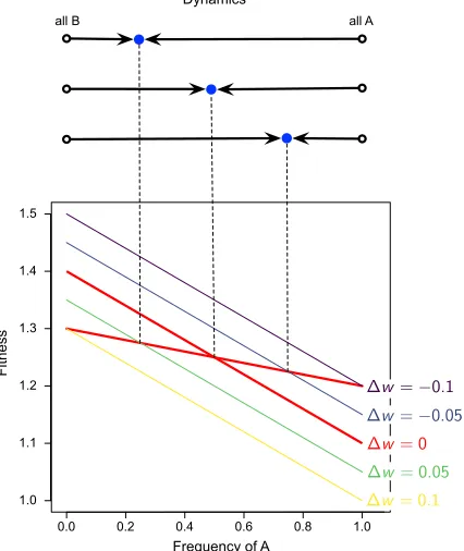
Figure 1: Change in the stable fixed point with change in baseline fitness
0.0 0.2 0.4 0.6 0.8 1.0
1.0 1.1 1.2 1.3 1.4 1.5
F
itn
ess
Frequency of A
all B all A
Dynamics
w= 0.1
w= 0 w= 0.05
w= 0.05
w= 0.1
Note: Initially,w0A=wB0 = 1. Then perturbations to the baseline fitness ofA, i.e.,∆w6= 0, lead to a change in the equilibrium levelˆx, i.e., intersection, at which stable coexistence is attained. Payoffs arepAA= 0.1,pAB= 0.4,
pBA= 0.2 andpBB= 0.3.
Figure 1 shows that the coexistence game is qualitatively robust against such per-turbations of the background fitness. For sufficiently small∆w =w0
B −w
0
A, there is a
different stable fixed point that still maintains the coexistence between the two subpopu-lations. Settingw¯A= ¯wBand solving forx, the stable fixed point is
ˆ
x= ∆w+pBB−pAB
pAA−pAB−pBA+pBB
. (7)
3. A population with age structure
We now consider the age-structured model in which both the relative abundance of types and individual age can affect the dynamics. As before, the population is very large, is not subject to density dependence, and its dynamics depend on relative frequencies of types. Individuals can survive from one step in time to the next, and, therefore, generations overlap. We takeAas the focal type to describe the dynamics. After the game, an A
individual of agejproduces a number
¯
Fj,A=Fj,A+πA(x) (8)
of offspring. Fertility is the sum of an age- and type-dependent componentFj,A>0and
the expected payoffπA(x), which changes with the relative abundancexofA. As payoffs
are strictly positive, we haveF¯j,A>0. Letnj,A(t)be the number ofAindividuals in age
classjattandnj,B(t)be the number ofBindividuals in age classjatt, with the total
subpopulations having sizeNA=Pjnj,AandNB=Pjnj,B, and the total population
beingN =NA+NB. Then, theAfraction of the population is
x(t) =
P
jnj,A(t)
P
jnj,A(t) +
P
jnj,B(t)
= NA(t)
NA(t) +NB(t)
=NA(t)
N(t) . (9)
Offspring enter the population in the next time step, to which the parent can survive with a survival probabilitySj,A, which again depends on age and type (but not on the
payoff). The dynamics of theAsubpopulation is then determined by
n1,A(t+ 1) n2,A(t+ 1)
.. . .. .
nω,A(t+ 1)
| {z }
nA(t+1) = ¯
F1,A(x) F¯2,A(x) . . . F¯ω−1,A(x) F¯ω,A(x) S1,A
S2,A
. ..
Sω−1,A
| {z }
¯
LA(x)
n1,A(t) n2,A(t)
.. . .. .
nω,A(t)
| {z }
nA(t)
(10)
Here,ω is the maximum age class thatAindividuals can reach. The vectornA(t)
represents the subpopulation state att. The matrixL¯A(t)is a population projection matrix
For technical purposes, we define the matrix
KA=
1 1 . . . 1 1 0 0 . . . 0 0 0 0 . . . 0 0
..
. ... . .. 0 0 0 0 0 0 0
(11)
which has the same dimensions asLA. A similar matrix is formed forB. We can then
write the dynamics of the abundances of the two subpopulations as
nA(t+ 1) = ¯LA(x)nA(t) = (LA+πA(x)KA)nA(t) (12a)
nB(t+ 1) = ¯LB(x)nB(t) = (LB+πB(x)KB)nB(t), (12b)
in which the matricesL¯AandL¯Bare split up into a frequency-independent part,LAand
LB, and a frequency-dependent part, πA(x)KA andπB(x)KB. The matricesLA and
LBare non-negative, as their entries are equal to or greater than zero, and can be shown
irreducible (Caswell 2001). Therefore, the Perron-Froebenius theorem applies and we can letλA be the Perron root ofLAandλB be the Perron root ofLB. As the effect of
expected payoffs is just to increase the value of some entries of these matrices,L¯A(x)
andL¯B(x)are also nonnegative and irreducible and have Perron roots¯λA(x)andλ¯B(x),
respectively.
Without the game, the population dynamics are simply
nA(t+ 1) =LAnA(t) (13a)
nB(t+ 1) =LBnB(t). (13b)
This linear case is within the scope of the ergodic theorem in demography (Cohen 1979). When a nonzero population state vector is repeatedly multiplied by a constant, non-negative and irreducible PPM, as in our case, the population state vector asymptot-ically becomes proportional to the leading right eigenvector of that PPM, and the pop-ulation grows at a rate equal to the Perron root of the PPM. Thus, asymptotically, the population sizes in the system in Equation (13) change as
assuming that the two population state vectors are proportional to the right leading eigen-vectors of the matricesL.
We assume that, initially, AandB have the same baseline vital rates, i.e.,LA =
LB, and that the population is initiated at x = x*. With equal expected payoffs, we
obtain L¯A(x∗) = ¯LB(x∗)with corresponding Perron roots at equilibrium λ¯A(x∗) =
¯
λB(x∗). Provided the two population state vectors are proportional to the right leading
eigenvectors of the respective matrices evaluated atx=x∗, the subpopulations ofAand B stably grow over time at the same rate. Thus, at the fixed point, we recover linear population dynamics
NA(t+ 1) = ¯λA(x∗)NA(t) (15a) NB(t+ 1) = ¯λB(x∗)NB(t). (15b)
We now introduce a small perturbation toA. In the presence of age structure, mu-tations can perturb one or more baseline vital rates of this type, but they do not change the number of age classes. As in the demographically unstructured model, we assume that mutations arise and go to fixation in the relevant subpopulation. We do not model the transient phase of population dynamics that starts when the mutation frequency be-comes non-negligible and, therefore, leads to a deviation from the game equilibrium and the demographic equilibrium, up to when the mutation becomes fixed, which requires the establishment of new game and demographic equilibria. Such modeling would involve the use of tools for the analysis of the transients in matrix population models (see, e.g., Fox and Gurevitch 2000; Yearsley 2004; Caswell 2007; Stott, Townley, and Hodgson 2011), which would make our model exceedingly complex. Instead we rely on mutant deviations that are sufficiently small so that a smooth passage from one equilibrium to another is guaranteed by stability of coexistence (see below and Appendix). We write
A0 to indicate that the type has mutated andLA0 to refer to the mutated baseline PPM.
The mutation is not neutral,λB−λA0 6= 0. In the absence of the game, the type whose
baseline projection matrix has the highest leading eigenvalue takes over. To understand whether the game can preserve coexistence we study the new system
nA0(t+ 1) = ¯LA0(x)nA0(t) = (LA0+πA0(x)KA0)nA0(t) (16a)
nB(t+ 1) = ¯LB(x)nB(t) = (LB+πB(x)KB)nB(t). (16b)
Note, however, thatπA0(x) =πA(x), as mutations affect only baseline vital rates.
We look for valuesxˆofxin(0, 1)such that the matricesL¯A0(ˆx)andL¯B(ˆx)have Perron
rootsλ¯A0(ˆx) = ¯λB(ˆx) = ¯λ(ˆx). In that case,A0andBcan coexist atxˆby having equal
population growth. This requires demographic stability, i.e.,nA0andnBare proportional
Finding whether such fixed points exist and are stable is of relevance for the evo-lution of demographic heterogeneity. Suppose that at the fixed point of the coexistence game a mutant appears in one subpopulation and the mutation reaches fixation within this subpopulation. Assume that a nearby alternative interior fixed point exists and is stable. Then this fixed point is reached. At this new fixed point, the population is demo-graphically heterogeneous. The two subpopulations have the same growth rate, yet their equilibrium PPMs differ for two reasons. First, the mutation has made some baseline vital rates different between types. Second, the expected payoffs betweenA0andBmust
be different in order to counteract the nonzero difference betweenλA0andλB.
4. Analysis
4.1 Interior fixed points
The interior fixed points of the dynamics in Equations (16) correspond to coexistences betweenA0andB. We assume such points are isolated. To retrieve them, we borrow from robust control theory applied to PPMs (Hodgson and Townley 2004; Hodgson, Townley, and McCarthy 2006). In this approach, one considers a PPM (say,Y) that is assumed non-negative and irreducible and, therefore, has a Perron root. A scalar amountδ >0is added to some entries ofY. A new matrix is obtained that can be represented as
˜
Y=Y+δpqT, (17)
wherepis a column vector andqT (hereT indicates vector transposition) is a row vector
such that the productpqT is a sparse matrix of0s and1s of the same dimensions asY,
where nonzero entries ofpqTcorrespond to entries ofYto whichδis added. AsY˜ is also
non-negative and irreducible, letzbe its Perron root. Following Hodgson and Townley (2004), we write the usual eigenvector problem for this matrix as
˜
Yc= (Y+δpqT)c=zc (18) for some nonzero eigenvectorc, which is guaranteed positive by the Perron-Froebenius theorem. Subtracting Yc on both sides, this equation becomes δpqTc = (zI
−Y)c. Ifz is not an eigenvalue ofY, the inverse of(zI−Y)exists. Multiplying on the left, first, by(zI−Y)−1and, then, by qT both sides of the equation, we obtain δqT(zI
−
Y)−1pqTc=qTc. Note thatqTcis a nonzero scalar. Dividing the equation byqTc, we
getδqT(zI
−Y)−1p= 1. LetG(z) =qT(zI
The functionG(z)is called the transfer function and is a rational function inz im-plicitly relatingδwithz(Hodgson and Townley 2004; Hodgson, Townley, and McCarthy 2006).
We can adopt this approach to capture exactly the effect of expected payoffs on the Perron roots ofLA0 andLB. The structure of the change induced by expected
pay-offs forA0 is represented byK
A0, which we can express by settingKA0 = pA0qTA0 =
[1, 0, 0, .., 0]T[1, 1, 1, .., 1]. The magnitude of the change is represented by the expected
payoffs so thatδ =πA0. We adopt the same procedure forB. We then write the
trans-fer functions for A0 as πA0qT
A0(zIA0 −LA0)−1pA0 = πA0GA0(z) = 1 and forB as πBqTB(zIB−LB)−1pB = πBGB(z) = 1. Using the definition of expected payoffs in
Equations (2) and solving forx, we can write for the two types
x= (GA0(z))
−1
−pAB pAA−pAB
(20a)
x= (GB(z))
−1
−pBB pBA−pBB
. (20b)
Equating these two expressions, we obtain
(pBA−pBB)[(GA0(z))−1−pAB] = (pAA−pAB)[(GB(z))−1−pBB]. (21)
This can be written as
pAApBB−pABpBA=
pAA−pAB GB(z) −
pBA−pBB GA0(z)
. (22)
The left side of this expression is the determinant of the payoff matrix det(M). Dividing through Equation (22) by this determinant, we get
1 = 1 det(M)
p
AA−pAB
GB(z) −
pBA−pBB GA0(z)
. (23)
The right side of this expression is a rational function in z. Any real root zˆof Equation (23) corresponds to the stable growth rate shared byA0 andB at fixed points
ˆ
xof the dynamics in Equation (16). Relevant roots ˆz must be strictly within ¯λB(0)
andλ¯B(1) so thatxˆ is constrained to the(0, 1) interval. The corresponding value of
ˆ
xfor some rootzˆcan be retrieved from either expression in Equation (20) by setting
are derived in the Appendix. These properties guarantee that when the system is at an initial stable fixed point andAmutates toA0, then a new nearby interior fixed point (if it exists) should be reached. A numerical example is given in Figure 2.
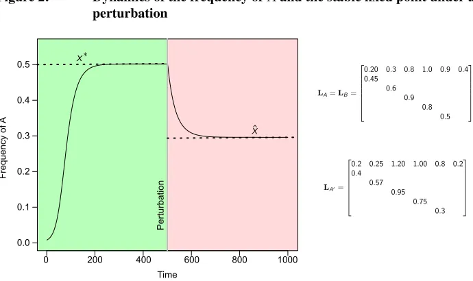
Figure 2: Dynamics of the frequency ofAand the stable fixed point under a perturbation
0 200 400 600 800 1000
0.0 0.1 0.2 0.3 0.4 0.5 Time F re qu en cy of A Pe rt urb at io n
LA=LB= 2 6 6 6 6 6 6 4
0.20 0.3 0.8 1.0 0.9 0.4 0.45 0.6 0.9 0.8 0.5 3 7 7 7 7 7 7 5
LA0=
2 6 6 6 6 6 6 4
0.2 0.25 1.20 1.00 0.8 0.2 0.4 0.57 0.95 0.75 0.3 3 7 7 7 7 7 7 5 x⇤ ˆ x
Note: A population in whichAandBhave equal vital rates (see inset PPM) is initiated and the dynamics ofxare followed for 1,000 time steps. Initial state vectors are[1, 1, 1, 1, 1, 1]TforAand994
6 [1, 1, 1, 1, 1, 1]
TforB. Initial
total population size is1, 000andx(0) = 6
1000. Neither subpopulation is at the stable age distribution implied by the common PPM. Att= 500,Ais mutated toA0(see inset PPM). Payoffs arepAA = 0.1,pAB = 0.4,
pBA= 0.2andpBB= 0.3.
4.2 Fixed-point sensitivity
The model in Equation (23) is challenging to analyze with respect to a specific perturba-tion that changesLA intoLA0. However, it is possible to formulate a simpler,
approxi-mate model similar to Equation (7), provided successive mutations that lead fromAtoA0
affect only a single vital rate and are of small effect, and expected payoffs are also small. Consider the initial scenario in whichAandBhave identical vital rates. Define the matrixLwith nonzero entriesSj = Sj,A = Sj,B andFj = Fj,A = Fj,B and Perron
rootλ=λA=λBwith corresponding right (column)uand left (row)vT eigenvectors
normalized so thatPjuj = 1andvTu= 1. The vectoruis proportional to the stable age
value vector, as itsj component is proportional to the relative contribution made to the future population by individuals of agej(Caswell 2001). Define the matrixK=KA=
KB. Suppose that some entries ofLdepend on a parameterθso that we can writeL(θ).
Differentiating the eigenvector equationλ=vTL(θ)uwith respect toθand evaluating at θ= 0while eigenvectors are assumed constant leads to
∂λ ∂θ
θ=0=vT∂
L
∂θ
θ=0u, (24) which corresponds to a classic result (Caswell 2001). We can use Equation (24) for two purposes. First, we can capture the linear change inλdue to expected payoffs by setting
θ=π. Then,
L(π) =
F1+π F2+π . . . Fω+π S1
. ..
Sω−1
(25)
and the sensitivity ofλto expected payoffs is
∂λ ∂π
π=0=vT∂
L
∂π
π=0u=vTKu=v1. (26)
Second, we can use Equations (24) and (26) to get an expression for the sensitivity of the initial fixed point to mutations in one type. Using Equation (26), we have that, to a linear approximation, the Perron root ofL¯A(x) = LA+πA(x)Kisλ¯A(x) ≈ λA+ v1πA(x)and the Perron root ofL¯B(x) = LB +πB(x)Kisλ¯B(x) ≈λB+v1πB(x).
Therefore, at a fixed point of the dynamics in Equation (15), we have
λA+v1πA(ˆx)≈λB+v1πB(ˆx) (27)
solving this forxˆby using Equation (2),
ˆ
x≈vλB−λA+v1(pBB−pAB)
1(pAA−pAB−pBA+pBB)
. (28)
At the initial fixed point (i.e., prior to perturbations on either type),λB−λA= 0and
Equation (28) is exact, as it gives the fixed pointxˆ=x∗. To understand the effect that a
Equation (28) with respect toθ. We do so by treatingv1 as constant. We also keep in
mind that the perturbation involves onlyAand, therefore,λBis not a function ofθ. We
then obtain an expression for the fixed-point sensitivity to the perturbation
∂x ∂θ
θ=0≈ −
1
v1(pAA−pAB−pBA+pBB) ∂λ ∂θ
θ=0. (29)
Note that the denominator in this expression is negative and, therefore,
∂x ∂θ
θ=0∝
∂λ ∂θ
θ=0. (30)
We can thus linearly approximate the new fixed point that pertains to the dynamics in Equation (16) after the perturbation from the initial equilibrium x∗ whereAandB
have identical vital rates as
ˆ
x≈x∗− θ
v1(pAA−pAB−pBA+pBB) ∂λ ∂θ
θ=0. (31)
We further assume that the mutation perturbs fertilities in an additive fashion, while it perturbs survival in a multiplicative fashion, as usual in population genetic models with age structure (Charlesworth 1994), and that the perturbation is limited to a single vital rate. Then, using Equation (24),
∂λ ∂θ
θ=0=
(
v1uj, if perturbation is onFj vj+1ujSj, if perturbation is onSj,
(32)
as shown in (Caswell 1978). A classical result in evolutionary demography about the relative magnitudes of these derivatives in populations that are not decreasing in size is
v1uj≥v1uj+1 (33)
vj+1ujSj≥vj+2uj+1Sj+1 (34)
(Hamilton 1966; Charlesworth 1994; Caswell 2001).
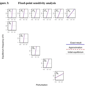
(31) to each nonzero entry of a projection matrixLAwhile keeping the initially identical
matrixLB constant. Figure 3 shows that the fixed point is less sensitive to late life, as
opposed to early life perturbations in vital rates.
Figure 3: Fixed-point sensitivity analysis
−0.3 0.0 0.2
0
0.5
1
−0.3 0.0 0.2
0
0.5
1
−0.3 0.0 0.2
0
0.5
1
−0.3 0.0 0.2
0
0.5
1
−0.3 0.0 0.2
0
0.5
1
−0.3 0.0 0.2
0
0.5
1
−0.3 0.0 0.2
0
0.5
1
−0.3 0.0 0.2
0
0.5
1
−0.3 0.0 0.2
0
0.5
1
−0.3 0.0 0.2
0
0.5
1
−0.3 0.0 0.2
0 0.5 1 Eq ui lib riu m fre qu en cy of A Perturbation Exact result Approximation Initial equilibrium
F1 F2 F3 F4 F5 F6
S1
S2
S3
S4
S5
Note: The fixed pointxˆis plotted as a function of the perturbation in a single vital rate of typeA, separately for each vital rate, whileBis kept unperturbed. Entries of the PPM ofAandBare those in the shared PPM in Figure 2. Payoffs arepAA= 0.01,pAB= 0.04,pBA= 0.02andpBB= 0.03.
5. Numerical exploration
5.1 Pleiotropy
pleiotropy. In addition, mutations can hit either typeA orB, and the magnitude may not always be small, as it is required to be by the model in Equation (31). Vital rate perturbations of this kind appear to be of particular interest for the study of demographic heterogeneity, as they should lead to a higher demographic diversity between the two types compared to perturbations limited to a single vital rate. Instead of using the ap-proximate model of the previous section, here we numerically explore the exact model in Equation (23) to understand more precisely how much demographic heterogeneity the stable coexistence game can tolerate without one type dominating the other when both subpopulations separately incorporate pleiotropic mutations.
To this aim, we parametrize the set of baseline vital rates that are initially shared betweenAandB. Survival follows a Gompertz mortality function, which is commonly used to model mammalian mortality (Gage 1998, 2001). In continuous time, Gompertz mortality at agetisµ(t) =aebtwherea >0gives baseline mortality andbis the rate of
aging. In discrete time, this translates to
Sj=exp
−
Z j+1
j
µ(y)dy
=exp
−
Z j+1
j
aebydy
=exph−a
b
eb(j+1)
−ebji.
(35)
Survival can either decline(b >0), improve(b <0), or stay constant(b= 0)with age. As for fertility, we set
Fj =cj(ω+ 1−j)2, (36)
whereω is the last age class. Thus, fertility is a third-degree polynomial inj, similar to that commonly used to model primate fertility (Gage 1998). With fixedc >0,Fj is
positive at all ages, increases from age1 to a peak at some intermediate age, and then declines to the last age class.
Figure 4: Regions of stable coexistence between two types under pleiotropic mutations
0.05 0.10 0.15 0.20 0.25 0.30
0.02
0.04
0.06
0.08
0.10
0.05 0.10 0.15 0.20 0.25 0.30
0.02
0.04
0.06
0.08
0.10
0.02 0.04 0.06 0.08 0.10
0.02
0.04
0.06
0.08
0.10
0.05 0.10 0.15 0.20 0.25 0.30
0.05 0.10 0.15 0.20 0.25 0.30
0.05 0.10 0.15 0.20 0.25 0.30
0.05 0.10 0.15 0.20 0.25 0.30
0.02 0.04 0.06 0.08 0.10
0.05 0.10 0.15 0.20 0.25 0.30
0.02 0.04 0.06 0.08 0.10
0.05 0.10 0.15 0.20 0.25 0.30
0.05 0.10 0.15 0.20 0.25 0.30
0.05 0.10 0.15 0.20 0.25 0.30
0.05 0.10 0.15 0.20 0.25 0.30
0.05
0.10
0.15
0.20
0.25
0.30 bA=bB= 0.2
cA=cB= 0.05
aA=bB= 0.2
cA=cB= 0.05
aA=bA=bB= 0.2
cB= 0.05
bA=aB= 0.2
cA=cB= 0.05
aA=aB= 0.2
cA=cB= 0.05
aA=bA=aB= 0.2
cB= 0.05
bA=aB=bB= 0.2
cA= 0.05
aA=aB=bB= 0.2
cA= 0.05
aA=bA=aB=bB= 0.2
aA bA cA
cB
bB
aB
Note: The shaded area indicates regions of stable coexistence betweenAandBfor the given parameter combina-tions. Payoffs arepAA= 0.1,pAB= 0.4,pBA= 0.2, andpBB= 0.3. Here there are alwaysωA=ωB= 6
age classes.
5.2 Cohort mortality
The average mortality in a cohort of same-age individuals from a demographically het-erogeneous population differs from the mortalities observed in cohorts from composing subpopulations (Curtsinger et al. 1992; Vaupel and Carey 1993; Chen, Zajitschek, and Maklakov 2013; Vaupel and Yashin 1985). Here we show that interesting patterns of av-erage cohort mortality can be retrieved from points inside coexistence regions like those explored in the previous section. Each point in this region represents a population that is characterized by a certain equilibrium frequencyxˆ ofA individuals and by the two projection matrices ofAandB evaluated at equilibrium. In both subpopulations, age-specific mortality follows a Gompertz function (defined above), possibly with different values for the parametersaandbbetween the two subpopulations. To observe the average mortality in a cohort of age 1 individuals that are sampled from this population, we adapt the methods of Vaupel and Yashin (1985). From the equilibrium projection matrices of
AandB, we compute the respective equilibrium birth ratesmA andmB. Here, mis
defined as the stable fraction of individuals that, at each time step, enter the first age class at demographic stability. Thus, if at demographic stabilityuj is the stable fraction of
individuals in age classjandFjis the number of individuals in age class1att+ 1per
individual in age classjatt,
m=X
j
ujFj. (37)
The initial fraction of age 1 individuals of typeAat demographic stability is
ϑ1=
ˆ
xmA
ˆ
xmA+ (1−xˆ)mB
, (38)
the remaining fraction1−ϑ1being of typeB. We then look at mortality in the cohort of
individuals of age 1 composed of a fractionϑ1ofAand a fraction(1−ϑ1)ofB. The
proportionpA(y)of theAsubcohort that survives at least to ageyis exp −
Ry
1 µA(t)dt
. The corresponding parameter forB,pB(y), is found analogously. When our cohort is of
agey, the fraction ofAindividuals is
ϑy=
ϑ1pA(y)
ϑ1pA(y) + (1−ϑ1)pB(y)
, (39)
and average mortality atyin the cohort is
¯
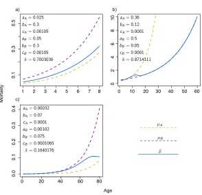
Figure 5: Average cohort mortality at coexistence
1 2 3 4 5 6 7 8
0.1
0.3
0.5
0 10 20 30 40 50 60
0 2 4 6 8 10
0 20 40 60 80
0.0 0.1 0.2 0.3 0.4
a) b)
c)
µB µA
¯
µ
aA= 0.025
bA= 0.3
cA= 0.00105
aB= 0.05
bB= 0.3
cB= 0.00105
ˆ
x= 0.7003036
aA= 0.36
bA= 0.12
cA= 0.0001
aB= 0.5
bB= 0.05
cB= 0.0001
ˆ
x= 0.8714111
aA= 0.00032
bA= 0.07
cA= 0.0001
aB= 0.00102
bB= 0.075
cB= 0.0001065
ˆ
x= 0.1640176
Mo
rt
al
ity
Age
Note: The mortality forAandB(dashed lines) is plotted against age, up to the maximum attainable age, together with the average mortality (continuous line) in a cohort composed of a mixture ofAandB. Both types have the same maximum age. The initial cohort composition is a function of the equilibrium fractionˆxofAand the birth rates ofAandBat coexistence. Payoffs arepAA= 0.1,pAB= 0.4,pBA= 0.2andpBB= 0.3.
6. Conclusions
The emergence and maintenance of demographic heterogeneity in a population can be explained by some form of frequency-dependent selection (Le Cunff, Baudisch, and Pak-daman 2013). Le Cunff, Baudisch, and PakPak-daman (2013) used stochastic agent-based simulations to show that types with discrete generations that differently allocate resources between survival and reproduction along their life may have equal fitness. For example, in their model, individuals that invest in early reproduction have a selective advantage in the first part of life over individuals that invest in early survival; in late life, the situ-ation is reversed. An important numerical result of Le Cunff, Baudisch, and Pakdaman (2013) is that, in a population with an initially random distribution of allocation strate-gies, frequency-dependent selection eventually produces a quasi-stationary distribution of types. The average mortality in a cohort of individuals from the quasi-stable popula-tion qualitatively resembles that observed in cohorts of captive organisms and in humans (Le Cunff, Baudisch, and Pakdaman 2013).
In Le Cunff, Baudisch, and Pakdaman (2013), however, the initial population is as-sumed heterogeneous, and generations are not overlapping. Some questions are then left unanswered: How can a population become heterogeneous in the first place? Can types with different survival and reproductive strategies also stably coexist when generations overlap? When generations overlap, does the age distribution of the population play a role in the dynamics of demographic heterogeneity? In the present study, we addressed the first two open questions. As for the third, we simply note here that there may be non-intuitive consequences of selection on different fitness components in finite populations, depending on the initial stable age distribution (Li et al. 2016).
demographic heterogeneity is not necessarily connected with fixed heterogeneity, as we assume, and other forms of heterogeneity may play a role, as reviewed in the introduction section.
With regard to the second question, we showed that with overlapping generations also, frequency-dependent selection can maintain demographic heterogeneity. Differently from Le Cunff, Baudisch, and Pakdaman (2013), in our framework we opted for a deter-ministic model in which fitness is identified with the population growth rate. As a draw-back, the presence of overlapping generations has complicated the analysis of our model. Therefore, we used numerical methods to find regions of coexistence under pleiotropic mutations. Using perturbation theory, we performed fixed-point sensitivity analysis to study how infinitesimal perturbations on single vital rates impact on the stable equilib-rium between types. Our analysis predicted a higher level of heterogeneity in late life. This may be somehow expected in the light of the classic result, indicating that selective dynamics in age-structured populations in a constant environment show diminished sen-sitivity to changes in late-life fitness components (Hamilton 1966; Charlesworth 1994; Caswell 2001). Yet it is relevant to see how a similar result can be derived from a game theoretical setting that represents a different context from the constant fitness scenario assumed in the derivation of this classic result. We have not considered the scenario in which the environment stochastically changes with time so that vital rates fluctuate in response to it. The population then has a stochastic growth rate (Tuljapurkar 1990). The analysis of this scenario is much more complicated, as it requires the sensitivities of the stochastic growth rate, which involve the second derivatives of the leading eigenvalue of the average projection matrix (Caswell 2001). As a consequence, the relationship be-tween fitness in early life and fitness in late life may also be less transparent than in the case of a constant environment (e.g., Orzack and Tuljapurkar 1989).
Interestingly, results based on pleiotropic mutations in our model can qualitatively mimic some mortality patterns that have been observed in natural and captive cohorts. This encourages us to further explore the potential of crossing demographic thinking with game theoretic approaches to explain patterns of mortality, and fertility, observed in nature.
7. Acknowledgments
References
Cam, E., Aubry, L.M., and Authier, M. (2016). The conundrum of heterogeneities in life history studies. Trends in Ecology and Evolution 31(11): 872–886. doi:10.1016/j.tree.2016.08.002.
Carey, J.R. and Judge, D.S. (2000). Mortality dynamics of aging.Generations24: 19–24.
Carey, J., Liedo, P., Orozco, D., and Vaupel, J. (1992). Slowing of mortal-ity rates at older ages in large medfly cohorts. Science 258(5081): 457–461. doi:10.1126/science.1411540.
Caswell, H. (1978). A general formula for the sensitivity of population growth rate to changes in life history parameters. Theoretical Population Biology14(2): 215–230. doi:10.1016/0040-5809(78)90025-4.
Caswell, H. (2001). Matrix population models. Sunderland: Sinauer Associates.
Caswell, H. (2007). Sensitivity analysis of transient population dynamics. Ecology Let-ters10(1): 1–15.doi:10.1111/j.1461-0248.2006.01001.x.
Chambon-Dubreuil, E., Auger, P., Gaillard, J.M., and Khaladi, M. (2006). Effect of aggressive behaviour on age-structured population dynamics. Ecological Modelling
193(3–4): 777–786.doi:10.1016/j.ecolmodel.2005.09.005.
Charlesworth, B. (1994). Evolution in age-structured populations. Cambridge: Cam-bridge University Press.
Charlesworth, B. and Partridge, L. (1997). Ageing: Levelling of the grim reaper.Current Biology7(7): R440–R442.doi:10.1016/S0960-9822(06)00213-2.
Chen, H., Zajitschek, F., and Maklakov, A.A. (2013). Why ageing stops: Heterogene-ity explains late-life mortalHeterogene-ity deceleration in nematodes. Biology Letters9(5): 1–4. doi:10.1098/rsbl.2013.0217.
Cohen, J.E. (1979). Ergodic theorems in demography. Bulletin of the American Mathe-matical Society (New Series)1(2): 275–295.
Cressman, R. (2003). Evolutionary dynamics and extensive form games. Cambridge: MIT Press.
Curtsinger, J., Fukui, H., Townsend, D., and Vaupel, J. (1992). Demography of geno-types: Failure of the limited life-span paradigm in drosophila melanogaster. Science
258(5081): 461–463.doi:10.1126/science.1411541.
Gage, T.B. (1998). The comparative demography of primates: With some comments on the evolution of life histories.Annual Review of Anthropology27: 197–221.
Gage, T.B. (2001). Age-specific fecundity of mammalian populations: A test of three mathematical models.Zoo Biology20(6): 487–499.doi:10.1002/zoo.10029.
Hamilton, W.D. (1966). The moulding of senescence by natural selection. Journal of Theoretical Biology12(1): 12–45.
Hodgson, D.J. and Townley, S. (2004). Methodological insight: Linking management changes to population dynamic responses: The transfer function of a projection ma-trix perturbation. Journal of Applied Ecology41(6): 1155–1161. doi:10.1111/j.0021-8901.2004.00959.x.
Hodgson, D.J., Townley, S., and McCarthy, D. (2006). Robustness: Predicting the effects of life history perturbations on stage-structured population dynamics.Theoretical Pop-ulation Biology70(2): 214–224. doi:10.1016/j.tpb.2006.03.004.
Hofbauer, J. and Sigmund, K. (1998). Evolutionary games and population dynamics. Cambridge: Cambridge University Press.
Horvitz, C.C. and Tuljapurkar, S. (2008). Stage dynamics, period survival, and mortality plateaus.The American Naturalist172(2): 203–215.
Huang, W., Haubold, B., Hauert, C., and Traulsen, A. (2012). Emergence of stable poly-morphism driven by evolutionary games between mutants.Nature Communications3: 919.
Kendall, B.E., Fox, G.A., Fujiwara, M., and Nogeire, T.M. (2011). Demographic het-erogeneity, cohort selection, and population growth. Ecology 92(10): 1985–1993. doi:10.1890/11-0079.1.
Kokko, H. (1997). Evolutionarily stable strategies of age-dependent sex-ual advertisement. Behavioral Ecology and Sociobiology 41(2): 99–107. doi:10.1007/s002650050369.
Kussel, E. and Leibler, S. (2005). Phenotypic diversity, population growth, and informa-tion in fluctuating environments.Science309(5743): 2075–2078.
Le Bras, H. (1976). Lois de mortalit´e et ˆage limite [laws of mortality and the life span].
Population31(3): 655–692.
Le Cunff, Y., Baudisch, A., and Pakdaman, K. (2013). How evolving heterogeneity distri-butions of resource allocation strategies shape mortality patterns.PLoS Computational Biology9(1): e1002825. doi:10.1371/journal.pcbi.1002825.
1: 1–18.
Li, X.Y., Giaimo, S., Baudisch, A., and Traulsen, A. (2015). Modeling evolutionary games in populations with demographic structure.Journal of Theoretical Biology380: 506–515.
Li, X.Y., Kurokawa, S., Giaimo, S., and Traulsen, A. (2016). How life history can sway the fixation probability of mutants.Genetics203: 1297–1313.
Maynard Smith, J. (1982). Evolution and the theory of games. Cambridge: Cambridge University Press.
Maynard Smith, J. (1986).The problems of biology. Oxford: Oxford University Press.
Maynard Smith, J. (1995). The theory of evolution. Cambridge: Cambridge University Press.
Maynard Smith, J. and Szathm´ary, E. (1995).The major transitions in evolution. Oxford: W.H. Freeman.
Meyer, C.D. (2015). Continuity of the Perron root.Linear and Multilinear Algebra63(7): 1332–1336.doi:10.1080/03081087.2014.934233.
Nowak, M.A., Sasaki, A., Taylor, C., and Fudenberg, D. (2004). Emergence of coopera-tion and evolucoopera-tionary stability in finite populacoopera-tions.Nature428: 646–650.
Nowak, M. (2006). Evolutionary dynamics. Cambridge: Harvard University Press.
Orzack, S. and Tuljapurkar, S. (1989). Population dynamics in variable environments: VII: The demography and evolution of iteroparity.American Naturalist133: 901–923.
Plard, F., Bonenfant, D., Delorme, D., and Gaillard, J. (2012). Modeling reproductive tra-jectories of roe deer females: Fixed or dynamic heterogeneity? Theoretical Population Biology82(4): 317–328. doi:10.1016/j.tpb.2012.03.006.
Promislow, D. (1991). Senescence in natural populations of mammals: A comparative study. Evolution45(8): 1869–1887.
Stearns, S. (1992).The evolution of life histories. Oxford: Oxford University Press.
Steiner, U.K. and Tuljapurkar, S. (2012). Neutral theory for life histories and individual variability in fitness components. Proceedings of the National Academy of Sciences
109(12): 4684–4689.doi:10.1073/pnas.1018096109.
Steinsaltz, D., Evans, S.N., and Wachter, K.W. (2005). A generalized model of mutation– selection balance with applications to aging. Advances in Applied Mathematics35(1): 16–33.doi:10.1016/j.aam.2004.09.003.
dynamics of population projection matrix models. Ecology Letters14(9): 959–970. doi:10.1111/j.1461-0248.2011.01659.x.
Traulsen, A. and Reed, F.A. (2012). From genes to games: Cooperation and cyclic dom-inance in meiotic drive.Journal of Theoretical Biology299: 120–125.
Tuljapurkar, S. (1990).Population dynamics in variable environments. Berlin: Springer.
Tuljapurkar, S., Steiner, U.K., and Orzack, S. (2009). Dynamic heterogeneity in life histories. Ecology Letters12(1): 93–106.doi:10.1111/j.1461-0248.2008.01262.x.
Vaupel, J.W. and Carey, J.R. (1993). Compositional interpretations of medfly mortality.
Science260(5114): 1666–1667. doi:10.1126/science.8503016.
Vaupel, J.W., Carey, J.R., Christensen, K., Johnson, T.E., Yashin, A.I., Holm, N.V., Ia-chine, I.A., Kannisto, V., Khazaeli, A.A., Liedo, P., Longo, V.D., Zeng, Y., Manton, K.G., and Curtsinger, J.W. (1998). Biodemographic trajectories of longevity. Science
280(5365): 855–860.doi:10.1126/science.280.5365.855.
Vaupel, J.W., Manton, K.G., and Stallard, E. (1979). The impact of heterogeneity in individual frailty on the dynamics of mortality. Demography 16(3): 439–454. doi:10.2307/2061224.
Vaupel, J.W. and Yashin, A.I. (1985). Heterogeneity’s ruses: Some surprising effects of selection on population dynamics. The American Statistician39(3): 176–185.
Wilson, A.J. and Nussey, D.H. (2010). What is individual quality? An evo-lutionary perspective. Trends in Ecology and Evolution 25(4): 207–214. doi:10.1016/j.tree.2009.10.002.
Yashin, A.I., Iachine, I.A., and Harris, J.R. (1999). Half of the variation in susceptibility to mortality is genetic: Findings from Swedish twin survival data. Behavior Genetics
29(1): 11–19. doi:10.1023/A:1021481620934.
Yashin, A.I., Vaupel, J.W., and Iachine, I.A. (1994). A duality in aging: The equivalence of mortality models based on radically different concepts. Mechanisms of Ageing and Development74(1): 1–14.doi:10.1016/0047-6374(94)90094-9.
Appendix
Linear stability
Here we establish the linear stability of interior fixed points of the dynamics in Equation (16). Along with the set of inequalities in (5), we also assume
pAA< pBA< pBB< pAB <1, (41)
so that payoffs make a limited contribution to fitness. First of all,uj,A0(t) =nNj,A0
A0 (t)and
uj,B(t) = nj,B
NB (t), i.e., the current fractions of theAandBsubpopulations in age class j. Then, using Equation (10), we write a dynamic equation forx, which is now theA0
fraction of the population, and we implicitly define a functionf(x(t)),
x(t+ 1) = NA0(t+ 1)
NA0(t+ 1) +NB(t+ 1)
=
P
jnj,A0(t)( ¯Fj,A0(t) +Sj,A0)
P
jnj,A0(t)( ¯Fj,A0(t) +Sj,A0) +
P
jnj,B(t)( ¯Fj,B(t) +Sj,B)
=
x(t)N(t)P
juj,A0(t)( ¯Fj,A0(t) +Sj,A0)
x(t)N(t)P
juj,A0(t)( ¯Fj,A0(t) +Sj,A0) + (1−x(t))N(t)
P
juj,B(t)( ¯Fj,B(t) +Sj,B)
= x(t)WA0(t)
x(t)WA0(t) + (1−x(t))WB(t)
| {z }
f(x(t))
,
(42)
where it is assumed thatSω,A=Sω,B= 0and whereWA0(t) =Pjuj,A0(t)( ¯Fj,A0(t) + Sj,A0)andWB(t) =Pjuj,B(t)( ¯Fj,B(t) +Sj,B). To simplify notation, we set
M(t) =x(t)WA0(t) + (1−x(t))WB(t). (43)
We differentiateW using Equations (2) and (8),
∂WA0 ∂x =
X
j
uj,A0(pAA−pAB) = (pAA−pAB)
X
j
uj,A0 =pAA−pAB, (44)
and, similarly,
∂WB ∂x =
X
j
uj,B(pBA−pBB) = (pBA−pBB)
X
j
uj,B =pBA−pBB. (45)
∂M
∂x =WA0+x(pAA−pAB) +pBA−pBB−WB−x(pBA−pBB), (46)
and, finally,
∂f ∂x =
1
M2
M(WA0+xpAA−xpAB)−xWA0∂M ∂x
. (47)
We evaluate this expression at some interior equilibriumx(t) = ˆxrecalling that, at this equilibrium, we also have demographic stability and, therefore, NA(t + 1) =
¯
λ(ˆx)NA(t)andNB(t+ 1) = ¯λ(ˆx)NB(t)where¯λ(ˆx) = ¯λA(ˆx) = ¯λB(ˆx)is the leading
eigenvalue shared byL¯A0(ˆx)andL¯B(ˆx). Hence, asWA0(ˆx) =WB(ˆx) = ¯λ(ˆx), ∂f
∂x
x=ˆx= 1 + ˆ
x(1−xˆ)(pAA−pAB−pBA+pBB)
¯
λ(ˆx) . (48)
Because of the inequalities in (5) and (41),
−1< pAA−pAB−pBA+pBB<0. (49)
Note also that in Equation (48) we should haveλ¯≥1(ˆx), as it makes sense to focus only on populations that are not going extinct, i.e., geometric growth per time unit should not be smaller than unity. Thus,
0< xˆ(1¯−xˆ) λ(ˆx) <
1
4, (50)
and
1−1 4 <
∂f ∂x
x=ˆx<1. (51)
We then conclude that the interior fixed pointx = ˆxis linearly stable. We have assumed thatA0andBmay have different vital rates. However, the same result holds for AandBwhen the two types share the same vital rates. This means that when the system is at an initial stable fixed point andAmutates toA0, a new nearby interior fixed point (if
it exists) should be reached. A numerical example is given in Figure 2.
Existence and uniqueness
point. Then there are at least two distinct interior fixed points, say,xˆ1andxˆ2withxˆ1<
ˆ
x2. By our stability result,1−14 < ∂x∂f|x=ˆx1 <1and1−
1
4 <
∂f
∂x|x=ˆx2<1. Therefore,
there is some0< hxˆ2−xˆ1such thatf(ˆx1+h)<xˆ1+handf(ˆx2−h)>xˆ2−h.
By the intermediate value theorem, f must have at least one other fixed point, say,xˆ3
betweenxˆ1andxˆ2and such that∂x∂f|x=ˆx3 >1. But this means thatxˆ3is linearly unstable
contradicting the fact that every interior fixed point off is linearly stable. Therefore, if a stable interior fixed point exists, then it is unique.
The Perron root of a matrix is continuous in the matrix entries (Meyer 2015). The Perron roots λ¯A(x)and ¯λB(x)are continuous in their respective entries F¯j,A(x)and
¯
Fj,B(x), which in turn are continuous in xvia expected payoffs. Hence, λ¯A(x)and
¯
λB(x)are continuous inxand, by the intermediate value theorem, the function¯λA(x)−
¯
λB(x)has at least one root in the(0, 1)interval when the following condition holds
sgn ¯λA0(0)−¯λB(0)
6
=sgn ¯λA0(1)−¯λB(1)
, (52)
where sgn(·)is the sign function. This condition is sufficient for the existence of a unique interior fixed point in our system in Equation (16), but it is not necessary. If the condition is false, the functionλ¯A(x)−λ¯B(x)may still have a root, provided that thexaxis is