A NEW FRAMEWORK FOR FLOODING CONTROL
IN REGULATED RIVER SYSTEMS
by
Elizabeth A. Kanashiro
A thesis
submitted in partial fulfillment of the requirements for the degree of Master of Science in Civil Engineering
Boise State University
DEFENSE COMMITTEE AND FINAL READING APPROVALS
of the thesis submitted by
Elizabeth A. Kanashiro
Thesis Title: A New Framework for Flooding Control in Regulated River Systems Date of Final Oral Examination: 10 December 2010
The following individuals read and discussed the thesis submitted by student Elizabeth A. Kanashiro, and they evaluated her presentation and response to questions during the final oral examination. They found that the student passed the final oral examination.
Arturo S. Leon, Ph.D. Chair, Supervisory Committee Murgel George, Ph.D. Member, Supervisory Committee Venkataramana Sridhar, Ph.D. Member, Supervisory Committee
The author gratefully acknowledge the financial support of the NSF Idaho EP-SCoR Program and the National Science Foundation under award number EPS-0814387.
This thesis presents a case study on the application of a dynamic framework for the intelligent control of flooding in the Boise River system in Idaho. This framework couples a robust and numerically efficient hydraulic routing approach with the popular multi-objective, non-dominated Sorting Genetic Algorithm II (NSGA-II). The novelty of this framework is that it allows for controlled flooding when the conveyance capacity of the river system is exceeded or is about to exceed. Controlled flooding is based on weight factors assigned to each reach of the system depending on the amount of damage that would occur should a flood occur. For example, an urban setting would receive a higher weight factor than a rural or agricultural area. The weight factor for a reach doesn’t need to be constant as it can be made a function of the flooding volume (or water stage) in the reach. The optimization algorithm minimizes flood damage by favoring low weighted floodplain areas (e.g., rural areas) rather than high weighted areas (e.g., urban areas) for the overbank flows. The proposed framework has the potential to improve water management and use of flood-prone areas in river systems, especially of those systems subjected to frequent flooding. The Hydraulic Performance Graph (HPG) of a channel reach graphically summarizes the dynamic relation between the flow through and the stages at the ends of the reach under gradually varied flow (GVF) conditions, while the Volume Performance Graph (VPG) summarizes the corresponding storage. The Rating Performance Graph (RPG) summarizes the dynamic relation between the flow through and the stages at the ends of the in-line structure under gradually varied flow or rapidly varied flow
robust and numerically efficient model because the hydraulics for all river reaches are pre-computed (i.e., any error attained during the computation of the water profiles for each reach-e.g., due to instability-can be detected and therefore corrected before the river system routing) and most of the computations for the system routing involve only interpolation steps. The latter makes this approach highly numerically efficient. The proposed framework is the first model of its kind that uses the HPG/VPG/RPG approach for intelligent control of river flooding and has been applied to the Boise River system of Idaho. In order to test the hydraulic routing approach, a model for unsteady flow routing through dendritic and looped river networks based on performance graphs is presented in this thesis. The application presented in this thesis is limited to subcritical flows; however, it can be extended to supercritical flows. The model builds upon the application of Hydraulic Performance Graph (HPG) to unsteady flow routing introduced by [12] and adopts the Volume Performance Graph (VPG) introduced by [16]. The HPG of a channel reach graphically summarizes the dynamic relation between the flow through and the stages at the ends of the reach under gradually varied flow (GVF) conditions, while the VPG summarizes the corresponding storage. Both, the HPG and VPG are unique to a channel reach with a given geometry and roughness, and can be computed decoupled from unsteady boundary conditions by solving the GVF equation for all feasible conditions in the reach. Hence, in the proposed approach, the performance graphs can be used for different boundary conditions without the need to recompute them. Previous models based on the performance graph concept were formulated for routing through single channels or channels in series. The new approach expands on the use of HPG/VPGs and adds the use of rating performance graphs for unsteady flow routing in dentritic
looped network and contrast its simulation results with those from the well-known unsteady HEC-RAS model. Our results show that the present extension of application of the HPG/VPGs appears to inherit the robustness of the HPG routing approach in [12].
ABSTRACT . . . . v
LIST OF TABLES . . . . xi
LIST OF FIGURES . . . . xii
LIST OF ABBREVIATIONS . . . . xx
LIST OF SYMBOLS . . . . xxii
1 Introduction . . . . 1
2 Unsteady flow routing model for complex river networks based on HPG and VPG: UNHVPG . . . . 13
2.1 Integration and Linking of Modules . . . 17
2.1.1 Module I: Definition of a River Network . . . 18
2.1.2 Module II: Computation of HPGs and VPGs . . . 20
2.1.3 Module III: Initial Conditions . . . 21
2.1.4 Module IV: Boundary Conditions . . . 21
2.1.5 Module V: Evaluation of Time Step (∆t) . . . 25
2.1.6 Module VI: River System Hydraulic Routing . . . 26
2.2 Application to a Looped River Network . . . 33
2.2.1 Case 1: Slow Flood-Wave . . . 37
3 Intelligent control of river flooding . . . . 50
3.1 Components of the Proposed Framework . . . 50
3.1.1 Optimization Component: The Non-Dominated Sorting Ge-netic Algorithm-II (NSGA-II) . . . 50
3.1.2 Simulation Component . . . 52
3.2 Integration and Linking of Components . . . 55
3.2.1 Module I: Representation of a River Network . . . 55
3.2.2 Module II: Computation of HPGs, VPGs, LFPGs, RFPGs, and RPGs . . . 57
3.2.3 Module III: Definition of Optimization Objectives and Con-straints for Flooding Control . . . 57
3.2.4 Module IV: Initial and Boundary Conditions . . . 60
3.2.5 Module V: River System Hydraulic Routing . . . 60
3.2.6 Module VI: Choose the Best Solution of Pareto . . . 61
3.3 Application of the Proposed Model to the Boise River System . . . 61
3.3.1 Hydrologic Modeling . . . 61
3.3.2 Optimization Objective and Constraints . . . 68
3.3.3 Initial and Boundary Conditions . . . 70
3.3.4 Results and Analysis of Scenarios . . . 73
4 Conclusions . . . . 85
REFERENCES . . . . 88
A Hydraulic Performance Graph . . . . 92
C Left Flooding Performance Graph . . . . 144
D Rigth Flooding Performance Graph . . . . 170
2.1 Geometric characteristics of river reaches of a looped river system . . . . 34 2.2 Comparison of CPU times for the simulation of cases 1 and 2. . . 42
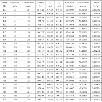
3.1 Geometric characteristics of Boise River reaches . . . 71
1.1 Schematic that illustrates the need for real-time control and the need
for accounting for system flow dynamics . . . 3
2.1 Example of a Hydraulic Performance Graph (HPG). . . 14
2.2 Example of a Volumetric Performance Graph (VPG). . . 15
2.3 Flow chart of the UNHVPG . . . 18
2.4 Schematic of a river reach . . . 20
2.5 Schematic of a node . . . 20
2.6 Schematic of an inline structure or gate node. . . 23
2.7 Schematic of a junction node . . . 24
2.8 Schematic of first interpolation case . . . 27
2.9 Schematic of second interpolation case . . . 27
2.10 Schematic of a simple network system . . . 30
2.11 Plan view of HEC-RAS looped river system. . . 35
2.12 Inflow hydrograph at node 1 for case 1: slow flood-wave. . . 36
2.13 Rating curve boundary at node 26 . . . 36
2.14 Flow hydrograph at downstream end of reaches 4 and 18 for case 1. . . . 38
2.15 Flow hydrographs at downstream end of reaches 9 and 26 for case 1. . . 38
2.16 Stage hydrographs at downstream end of reaches 4 and 18 for case 1. . . 39
2.17 Stage hydrographs at downstream end of reaches 9 and 26 for case 1. . . 39
for case 1. . . 41 2.19 Difference in water stages at downstream end of reaches 9 and 18 for
case 1. . . 41 2.20 Difference in conservation of volume at downstream end of reaches 9
and 18 for case 1. . . 42 2.21 Inflow hydrograph at node 1 for case 2: fast flood-wave. . . 43 2.22 Flow hydrographs at downstream end of reaches 4 and 18 for case 2. . . 43 2.23 Flow hydrographs at downstream end of reaches 9 and 26 for case 2. . . 44 2.24 Stage hydrographs at downstream end of reaches 4 and 18 for case 2. . . 44 2.25 Stage hydrographs at downstream end of reaches 9 and 26 for case 2. . . 45 2.26 Difference in flow discharges at downstream end of reaches 9 and 18
for case 2. . . 46 2.27 Difference in water stages at downstream end of reaches 9 and 18 for
case 2. . . 46 2.28 Difference in conservation of volume at downstream end of reaches 9
and 18 for case 2. . . 47 2.29 Flow discharge vs. water stage at downstream end of reach 18 for case 2. 47 2.30 Numerical accuracy of UNHVPG due to time discretization for the
upstream end of reach 14 and downstream end of reach 23 . . . 49
3.1 Flow chart of proposed framework for the intelligent control of river flooding. . . 51 3.2 Cross-section schematic for definition of left and right flooding volumes. 53 3.3 Schematic of Boise river’s plan view . . . 62
3.5 Plan view of major storage reservoirs in the Boise river basin. . . 65
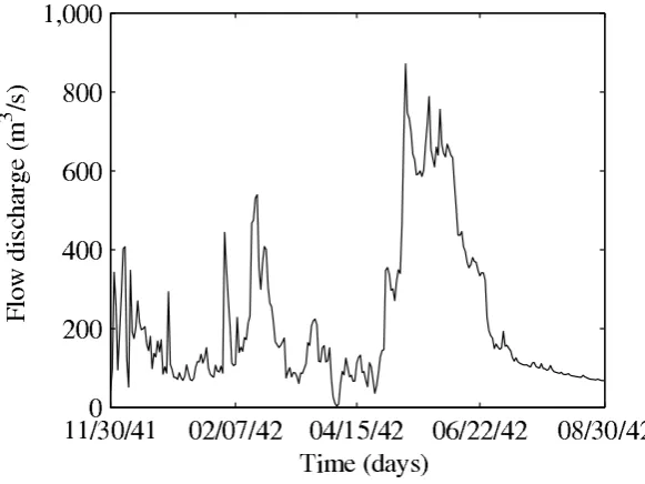
3.6 Inflow hydrograph subtracting active storage capacity of Anderson Ranch, Arrow Rock, Hubbard reservoirs and Lake Lowell. . . 67
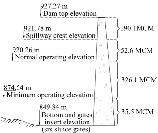
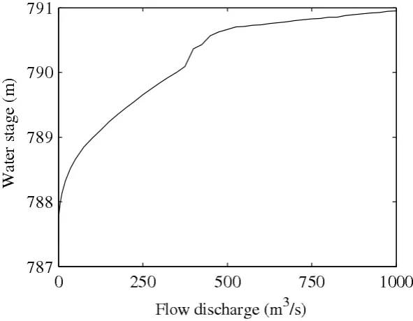
3.7 Stage-storage relationship of Lucky Peak reservoir. . . 68
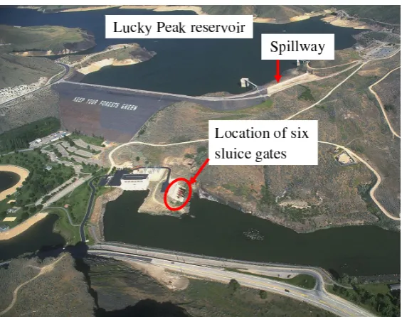
3.8 Plan view of Lucky Peak reservoir and associated structures. . . 70
3.9 Rating curve at most downstream end of river system (node J26). . . 72
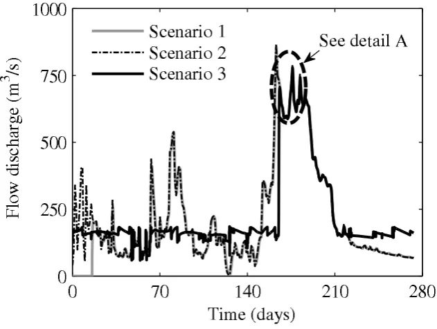
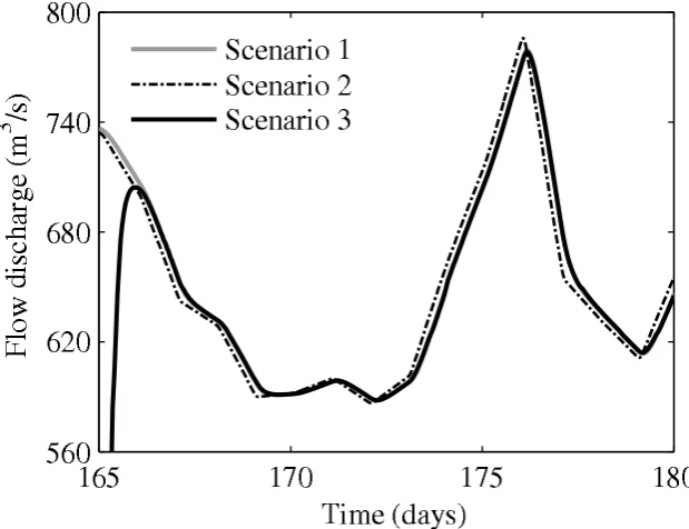
3.10 Flow hydrographs at downstream end of reach R1 for simulated scenarios. 74 3.11 Flow hydrographs at downstream end of reach R10 for simulated sce-narios. . . 74
3.12 Detail A in Figure 3.11. . . 75
3.13 Flow hydrographs at downstream end of reach R22 for simulated sce-narios. . . 75
3.14 Stage hydrographs at downstream end of reach R1 for simulated sce-narios. . . 76
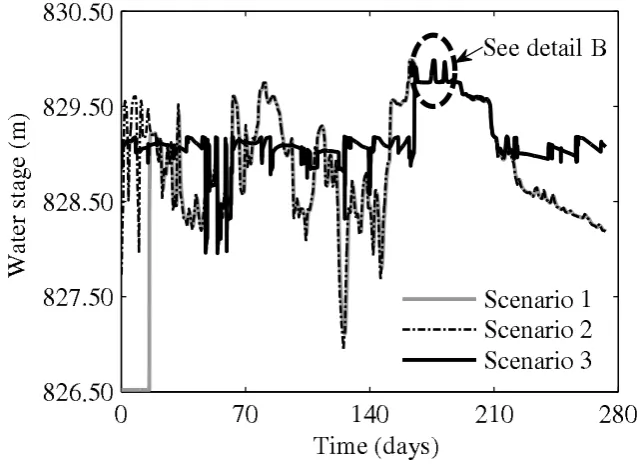
3.15 Stage hydrographs at downstream end of reach R10 for simulated scenarios. . . 76
3.16 Detail B in Figure 3.15. . . 77
3.17 Stage hydrographs at downstream end of reach R22 for simulated scenarios. . . 77
3.18 Peak flow at downstream end of reaches R1, R10 and R22 for scenario 2. 78 3.19 Peak flow at upstream end of reach R1 and at downstream end of reaches R10 and R22 for scenario 3. . . 79
3.20 Objective function 1 (Equation 3.1) for simulated scenarios. . . 81
3.21 Objective function 2 (Equation 3.2) for simulated scenarios. . . 81
3.23 Inflow, outflow, and water stage hydrographs at Lucky Peak reservoir. . 83
3.24 Operation of all gates (six) at Lucky Peak reservoir according to pro-posed framework. . . 83
3.25 Results of objective functions according to proposed framework (Equa-tion 3.1 and Equa(Equa-tion 3.2). . . 84
A.1 Hydraulic Performance Graph - Reach R1 . . . 93
A.2 Hydraulic Performance Graph - Reach R2 . . . 94
A.3 Hydraulic Performance Graph - Reach R3 . . . 95
A.4 Hydraulic Performance Graph - Reach R4 . . . 96
A.5 Hydraulic Performance Graph - Reach R5 . . . 97
A.6 Hydraulic Performance Graph - Reach R6 . . . 98
A.7 Hydraulic Performance Graph - Reach R7 . . . 99
A.8 Hydraulic Performance Graph - Reach R8 . . . 100
A.9 Hydraulic Performance Graph - Reach R9 . . . 101
A.10 Hydraulic Performance Graph - Reach R10 . . . 102
A.11 Hydraulic Performance Graph - Reach R11 . . . 103
A.12 Hydraulic Performance Graph - Reach R12 . . . 104
A.13 Hydraulic Performance Graph - Reach R13 . . . 105
A.14 Hydraulic Performance Graph - Reach R14 . . . 106
A.15 Hydraulic Performance Graph - Reach R15 . . . 107
A.16 Hydraulic Performance Graph - Reach R16 . . . 108
A.17 Hydraulic Performance Graph - Reach R17 . . . 109
A.18 Hydraulic Performance Graph - Reach R18 . . . 110
A.20 Hydraulic Performance Graph - Reach R20 . . . 112
A.21 Hydraulic Performance Graph - Reach R21 . . . 113
A.22 Hydraulic Performance Graph - Reach R22 . . . 114
A.23 Hydraulic Performance Graph - Reach R23 . . . 115
A.24 Hydraulic Performance Graph - Reach R24 . . . 116
A.25 Hydraulic Performance Graph - Reach R25 . . . 117
B.1 Volume Performance Graph - Reach R1 . . . 119
B.2 Volume Performance Graph - Reach R2 . . . 120
B.3 Volume Performance Graph - Reach R3 . . . 121
B.4 Volume Performance Graph - Reach R4 . . . 122
B.5 Volume Performance Graph - Reach R5 . . . 123
B.6 Volume Performance Graph - Reach R6 . . . 124
B.7 Volume Performance Graph - Reach R7 . . . 125
B.8 Volume Performance Graph - Reach R8 . . . 126
B.9 Volume Performance Graph - Reach R9 . . . 127
B.10 Volume Performance Graph - Reach R10 . . . 128
B.11 Volume Performance Graph - Reach R11 . . . 129
B.12 Volume Performance Graph - Reach R12 . . . 130
B.13 Volume Performance Graph - Reach R13 . . . 131
B.14 Volume Performance Graph - Reach R14 . . . 132
B.15 Volume Performance Graph - Reach R15 . . . 133
B.16 Volume Performance Graph - Reach R16 . . . 134
B.17 Volume Performance Graph - Reach R17 . . . 135
B.19 Volume Performance Graph - Reach R19 . . . 137
B.20 Volume Performance Graph - Reach R20 . . . 138
B.21 Volume Performance Graph - Reach R21 . . . 139
B.22 Volume Performance Graph - Reach R22 . . . 140
B.23 Volume Performance Graph - Reach R23 . . . 141
B.24 Volume Performance Graph - Reach R24 . . . 142
B.25 Volume Performance Graph - Reach R25 . . . 143
C.1 Left Flooding Performance Graph - Reach R1 . . . 145
C.2 Left Flooding Performance Graph - Reach R2 . . . 146
C.3 Left Flooding Performance Graph - Reach R3 . . . 147
C.4 Left Flooding Performance Graph - Reach R4 . . . 148
C.5 Left Flooding Performance Graph - Reach R5 . . . 149
C.6 Left Flooding Performance Graph - Reach R6 . . . 150
C.7 Left Flooding Performance Graph - Reach R7 . . . 151
C.8 Left Flooding Performance Graph - Reach R8 . . . 152
C.9 Left Flooding Performance Graph - Reach R9 . . . 153
C.10 Left Flooding Performance Graph - Reach R10 . . . 154
C.11 Left Flooding Performance Graph - Reach R11 . . . 155
C.12 Left Flooding Performance Graph - Reach R12 . . . 156
C.13 Left Flooding Performance Graph - Reach R13 . . . 157
C.14 Left Flooding Performance Graph - Reach R14 . . . 158
C.15 Left Flooding Performance Graph - Reach R15 . . . 159
C.16 Left Flooding Performance Graph - Reach R16 . . . 160
C.18 Left Flooding Performance Graph - Reach R18 . . . 162
C.19 Left Flooding Performance Graph - Reach R19 . . . 163
C.20 Left Flooding Performance Graph - Reach R20 . . . 164
C.21 Left Flooding Performance Graph - Reach R21 . . . 165
C.22 Left Flooding Performance Graph - Reach R22 . . . 166
C.23 Left Flooding Performance Graph - Reach R23 . . . 167
C.24 Left Flooding Performance Graph - Reach R24 . . . 168
C.25 Left Flooding Performance Graph - Reach R25 . . . 169
D.1 Rigth Flooding Performance Graph - Reach R1 . . . 171
D.2 Rigth Flooding Performance Graph - Reach R2 . . . 172
D.3 Rigth Flooding Performance Graph - Reach R3 . . . 173
D.4 Rigth Flooding Performance Graph - Reach R4 . . . 174
D.5 Rigth Flooding Performance Graph - Reach R5 . . . 175
D.6 Rigth Flooding Performance Graph - Reach R6 . . . 176
D.7 Rigth Flooding Performance Graph - Reach R7 . . . 177
D.8 Rigth Flooding Performance Graph - Reach R8 . . . 178
D.9 Rigth Flooding Performance Graph - Reach R9 . . . 179
D.10 Rigth Flooding Performance Graph - Reach R10 . . . 180
D.11 Rigth Flooding Performance Graph - Reach R11 . . . 181
D.12 Rigth Flooding Performance Graph - Reach R12 . . . 182
D.13 Rigth Flooding Performance Graph - Reach R13 . . . 183
D.14 Rigth Flooding Performance Graph - Reach R14 . . . 184
D.15 Rigth Flooding Performance Graph - Reach R15 . . . 185
D.17 Rigth Flooding Performance Graph - Reach R17 . . . 187
D.18 Rigth Flooding Performance Graph - Reach R18 . . . 188
D.19 Rigth Flooding Performance Graph - Reach R19 . . . 189
D.20 Rigth Flooding Performance Graph - Reach R20 . . . 190
D.21 Rigth Flooding Performance Graph - Reach R21 . . . 191
D.22 Rigth Flooding Performance Graph - Reach R22 . . . 192
D.23 Rigth Flooding Performance Graph - Reach R23 . . . 193
D.24 Rigth Flooding Performance Graph - Reach R24 . . . 194
D.25 Rigth Flooding Performance Graph - Reach R25 . . . 195
BC – Boundary Condition
CIB – Controlled In-line structure Boundary
CPU – Central Processing Unit
CWMS – Corps Water Management System
EBC – External Boundary Condition
GVF – Gradually Varied Flow
HEC– Hydrologic Engineering Center
HECFloodOpt– Hydrologic Engineering Center Reservoir Flood Control Optimiza-tion
HEC-RAS – Hydrologic Engineering Centers River Analysis System
HEC-ResSim – Hydrologic Engineering Center Reservoir Simulation
HEC-PRM – Hydrologic Engineering Center Prescriptive Reservoir model
HPG – Hydraulic Performance Graph
HPC – Hydraulic Performance Curve
IBC – Internal Boundary Condition
InflowHydro – Inflow hydrograph
LFPG – Left Flooding Performance Graph
NSGA-II – Non-dominated Sorting Genetic Algorithm II
RIBASIM – River Basin Simulation
RFPG – Right Flooding Performance Graph
RPG – Rating Performance Graph
SWAT – Soil and Water Assessment Tool
UNHVPG – Unsteady flow routing model for complex river networks based on HPG and VPG
VPG – Volume Performance Graph
A Constant (> 1)
c Coefficient
c Average gravity wave celerity
d Downstream end index
f Function
F V Flooding volume
G Discrete gate position
i Node index
I Inflow
∀i For all i
j River reach index
k Total number of river reaches linked to the node
max Maximum
min Minimum
n Discrete-time index
N Set of nodes
NB Set of downstream boundary nodes
O Outflow
p Number of outflowing river reaches linked to the node
Qdj Flow discharge at downstream end of reach j
QuCIBstorage of a river reach or reservoir located upstream of the CIB
Quj Flow discharge at upstream end of reach j
RR Total number of river reaches
s Slope
S Storage
∆t Time step
u Upstream end index
u Average reach velocity
v Number of inflowing river reaches linked to the node
V Cumulative outflow volume
w Weight factor
W S Water stage
∆x Length of river reach
ydj Water depth at downstream end of reachj
yuj Water depth at upstream end of reachj
zdj Channel bottom elevation at downstream end of reach j
zuj Channel bottom elevation at upstream end of reach j
CHAPTER 1
INTRODUCTION
River flooding is a recurrent threat that normally ensues a huge cost, both in terms of human suffering and economic losses associated with damage to infrastructure, loss of business, and the cost of insurance claims. From 2005 to 2009, the National Weather Service [28] estimated 63 billion dollars in losses in the U.S. associated with flooding. The catastrophic disasters associated with river flooding urge the re-evaluation of current strategies for flood control for most appropriate frameworks.
Recent studies on flood mitigation indicate that major emphasis must be given to flood control projects under the greater framework of basin-wide ecosystem rehabil-itation (e.g., [35], [6]). These studies also aim for improving structural measures for minimizing the impact of floods while emphasizing the importance of risk management in flood control projects. A review of common structural measures used for flood control (e.g., levees, dams) reveals most of these measures are passive (static), with dams being the most important structural measure for flood control (e.g., [37]).
system may have enough in-line storage capacity, while other portions of the system may be overflowing.
A flooding process may be highly dynamic and may start from anywhere in the river system ([26]). It may start from upstream (e.g., large inflows), downstream (i.e., high water levels at downstream), or laterally from the connecting reaches (e.g., water levels at river junctions near the reach banks). It may change for the same river system depending on inflows to the river system and antecedent boundary conditions. Accounting for system flow dynamics is also important because flow conveyance from one reservoir to another is not instantaneous but depends on the capacity of the connecting reaches, the capacity of associated gates, outlet structures, and the dynamic hydraulic gradients. Clearly, rule curves are insufficient for making system-wide operational decisions.
Figure 1.1: Schematic that illustrates the need for real-time control and the need for accounting for system flow dynamics
for making system-wide operational decisions.
for the same river system depending on inflows to the river system and antecedent boundary conditions. Accounting for system flow dynamics is also important because flow conveyance from one reservoir to another is not instantaneous but depends on the capacity of the connecting reaches, the capacity of associated gates, outlet structures, and the dynamic hydraulic gradients. The author is not aware of a single river system in the world that has a real-time flood control framework combining simulation and optimization to account for system flow dynamics.
Water Management System (CWMS). The RIBASIM (RIver BAsin SIMulation) [[7]] model is another comprehensive and flexible tool for reservoir operation. Since 1985, RIBASIM has been applied in more than 20 countries world wide and is used by a wide range of both national and regional agencies. RIBASIM enables the user to evaluate a variety of measures related to infrastructure, operational, and demand management in order to see results in terms of water quantity and flow composition.
Recently, many more combined simulation-optimization models were formulated for reservoir operation including flood control. [30] proposed to optimize the control strategies for the Hoa Binh reservoir operation. The control strategies were set up in the MIKE 11 simulation model to guide the releases of the reservoir system according to the current storage level, the hydro-meteorological conditions, and the time of the year. [23] refined an existing optimization/simulation procedure for rebalancing flood control and refill objectives for the Columbia River Basin for anticipated global warming. To calibrate the optimization model for the 20th century flow, the objective function was tuned to reproduce the current reliability of reservoir refill, while pro-viding comparable levels of flood control to those produced by current flood control practices. After the optimization model was calibrated using the 20th century, flow the same objective function was used to develop flood control curves for a global warming scenario.
models having the capability to perform hydraulic routing of any river system. In the authors experience, some of the existing routing models, especially those that are one-dimensional, are highly robust for a wide range of conditions. This is the first limitation of these models because they are not robust for all conditions. For instance, the widely known unsteady HEC-RAS model ([18]) provides accurate results for a large range of conditions but may fail for some others. It is pointed out that when the HEC-RAS model finds problems of convergence, the simulation is not stopped but rather continues assuming pre-specified conditions (e.g., critical flow). Certainly the results after the convergence problems cannot be trusted.
Most free surface flows (also called open-channel flows) are unsteady and non-uniform. Hence, in many applications the spatial and temporal variation of water stages and flow discharges need to be determined. Unsteady flows in river systems are typically simulated using one-dimensional models although two and three-dimensional models are now being used more frequently. In a one-dimensional framework, un-steady flows in rivers are typically simulated by the Saint-Venant equations, the pair of partial differential equations representing conservation of mass and momentum for a control volume are:
∂A ∂t +
∂Q
∂x = 0 (1.1)
1 g ∂V ∂t + ∂ ∂x ( V2 2g )
+ cosθ∂y
∂x +Sf −So = 0 (1.2)
slope and Sf = friction slope. In Eq. (1.2) [momentum equation], the first, second,
third, fourth, and fifth terms represent the local acceleration, convective acceleration, pressure gradient, friction, and gravity terms, respectively.
The Saint-Venant equations are typically solved for appropriate initial and bound-ary conditions to simulate the spatial and temporal variation of water stages and flow discharges resulting from flood routing. At present, no analytical solution for the Saint-Venant equations is known, except for special conditions (e.g., dam break flow over a dry bed in a frictionless and horizontal channel). Hence, solutions of general open-channel flow conditions such as those found in practical applications are sought numerically. Solutions to the full dynamic, one dimensional Saint-Venant Equations and their quasi-steady, noninertia (or diffusion), and kinematic wave approximations (details on these approximations can be found for example in [39]) have been sought based on several numerical schemes and methods (e.g., [1]). As emphasized in [12] and [14], despite the wide array of methods available for the solution of the Saint-Venant equations, the lack of robustness and accuracy issues still pose a problem.
take between five to ten minutes for performing the unsteady flow computations.
An important issue with unsteady flow models is computational burden, especially when an unsteady model is used for optimization problems such as real-time operation of regulated river systems (e.g., [25]). In this case, hundreds or even thousands of runs need to be performed for each operational decision (∼30 minutes), which would require numerically efficient models for unsteady flow routing or a large number of computer processors (clusters). Even if the simulations are run on computer clusters, there is no guarantee that hydraulic routing models will work for all ranges of conditions (e.g., low stage flows up to flows in the floodplains). In the authors’ experience, under some simulation conditions most of the existing routing models fail to converge to a solution. In particular, the widely known unsteady HEC-RAS model ([18]), which has been found to converge for a range of conditions, fails to converge under some conditions. When HEC-RAS fails to converge, it proceeds with the simulation based on assumed pre-specified conditions (e.g., critical flow), which may yield questionable results.
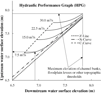
HPG shown in Figure 2.1 has few HPCs; in actual applications, the number of HPCs must be set based on a precision goal. This must be decided based on a convergence analysis, which consists of successive refinement of the resolution of the set of HPCs to a resolution such that the solution for the conditions of interest (e.g., stage and flow hydrographs at a given station) becomes nearly independent of the number of HPCs used. The procedure to determine the optimal resolution of HPCs to ensure that a prescribed accuracy is afforded is outside the scope of this thesis.
HPGs can be used to summarize gradually varied subcritical and supercritical flows. However, they have been mostly applied to summarize subcritical GVF in channel reaches with steep, mild, adverse, and horizontal slopes (see methodology in [40]; and [32]). The construction of the HPG for each reach may involve hundreds of GVF simulations, each simulation corresponding to one discrete point on the HPG. When using a one-dimensional model for constructing the performance graphs, any GVF model can be used. In the present application, the steady HEC-RAS model was used to generate the HPG’s/VPG’s.
to satisfy the reach-wise mass conservation during routing. The VPG approach is equivalent to enforcing Equation (1.1) [conservation of mass] in a reach (see details in [16]). An example of a VPG for a mild-sloped channel is depicted in Figure 2.2. The HPG and VPG are unique to a channel reach with a given geometry and roughness, and can be computed decoupled from unsteady boundary conditions by solving the GVF equation for all feasible conditions in the reach. They are essentially a fingerprint of all gradually varied flow conditions in a channel reach. Consequently, HPG/VPGs need to be revised only when geomorphic changes modify the geometry or roughness characteristics of the channel ([40]). A significant advantage of the HPG approach with respect to other routing models is that the results are little sensitive to space and time discretization ([12]).
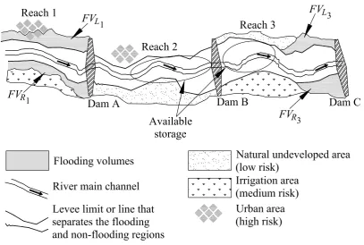
To address the complexity of river flooding and to overcome the limitations of current frameworks for flood control, a coupled optimization-simulation framework is proposed that accounts for system flow dynamics and that makes possible the intelligent control of river flooding (e.g., automatic operation of gates and locks in river systems). This framework is robust and enough fast so that it will allow its application to actual complex river systems in real-time.
The main benefit of the proposed framework is that it will maximize the in-line storage of the entire river system and it will allow controlled flooding only after the capacity of the river system has been exceeded. This controlled flooding will be based on weight factors assigned to each reach of the system depending on a hierarchy of risk to losses associated with flooding. Naturally, river reaches that are less prone to losses are assigned smaller weight factors and reaches that are more prone to losses are assigned larger weight factors.
model with a good simulation model, the proposed framework couples the well-known multi-objective, non-dominated Sorting Genetic Algorithm II (NSGA-II) with the concept of Hydraulic Performance Graph, Volume Performance Graph, and Rating Performance Graph.
This thesis is presented in two major parts, the first is the unsteady flow routing in complex river networks and the second is the intelligent control of river flooding.
The present work extends the application of the performance graph approach for unsteady flow routing in river networks. In a similar fashion to the unsteady approach of [12], the model introduced here, to which we refer to as UNHVPG model, assumes that the flow is timewise steady at the different time steps of the routing. The application presented in this thesis is limited to subcritical flows; however, it can be extended to supercritical flows. Besides relying on the HPG/VPG concept, the UNHVPG model also makes use of what we refer to as Rating Performance Graph (RPG). RPGs graphically summarize the dynamic relation between the flow through and the stages upstream and downstream of an in-line structure. RPG’s are conceptually similar to look-up tables such as those utilized to characterize the dynamics of hydraulic structures in the FEQ model of [10]. However, RPG’s are described with an adaptive spacing so as to capture changes smoothly, which leads to better interpolation estimates. Further details on RPGs are presented in the next section. Results of these models are compared and discussed in Chapter 2.
The Intelligent control of river flooding couples the hydraulic and optimization components of the proposed framework. This framework is applied to the Boise River system and results of this application are discussed in Chapter 3.
CHAPTER 2
UNSTEADY FLOW ROUTING MODEL FOR COMPLEX
RIVER NETWORKS BASED ON HPG AND VPG:
UNHVPG
This chapter presents a highly robust model for unsteady flow routing through den-tritic and looped river network. The application presented in this chapter is limited to subcritical flows; however, it can be extended to supercritical flows. The model builds upon the application of the Hydraulic Performance Graph (HPG) to unsteady flow routing introduced by Gonz´alez-Castro [12] and adopts the Volume Performance Graph (VPG) introduced by Hoy and Schmidt [16].
The hydraulic component of the proposed framework consists in dividing the river system into reaches and pre-computing the hydraulics for each of these reaches independently using any gradually varied flow model (one-, two-, or three-dimensional model). The pre-computed hydraulics for each reach is stored in matrices and is accessed as look-up tables. The Hydraulic routing adopted for each river reach is performed using the Hydraulic Performance Graph (HPG) and Volume Performance Graph (VPG).
depths at the ends of the channel reach for different constant discharges. A significant advantage of the HPG approach with respect to other routing models is that any error attained during the pre-computation of the hydraulics (e.g., due to instability) can be detected and therefore corrected before the optimization process (e.g., redo simulations with other discretization parameters). For a detailed description of HPGs, see Yen and Gonz´alez-Castro [40]. An example of an HPG and a VPG for a mild-sloped channel are depicted in Figures 2.1 and 2.2, respectively. These HPG and VPG intentionally show a few performance curves (constant discharge curves). In actual applications, the number of discharges must be commensurate to the desired interpolation precision.
Figure 2.2: Example of a Volumetric Performance Graph (VPG).
The HPG of a channel reach graphically summarizes the dynamic relation between the flow through and the stages at the ends of the reach under gradually varied flow (GVF) conditions, while the VPG summarizes the corresponding storage. Both the HPG and VPG are unique to a channel reach with a given geometry and rough-ness, and can be computed decoupled from unsteady boundary conditions by solving the GVF equation for all feasible conditions in the reach. Hence, in the proposed approach, the performance graphs can be used for different boundary conditions without the need to recompute them. Previous models based on the performance graph concept were formulated for routing through single channels or channels in series.
a channel reach. Consequently, HPG/VPGs need to be revised only when geomorphic changes modify the geometry or roughness characteristics of the channel ([40]). The HPG/VPG are obtained for as many flows and downstream boundary conditions as necessary to cover the region of possible pairs of upstream and downstream stages in the channel reach.
The performance graphs approach applies to flow routing when the local acceler-ation is negligible. This condition is met by flows in many natural and man-made systems [[15] showed that the local acceleration term is small compared to the gravity and friction terms even for a steep river with a “very fast-rising flood”]. Actually, the relative contribution of the local acceleration with respect to the pressure gradient is in the order of the Froude number squared ([15]). Typically, the maximum Froude number of mild-slope unregulated river systems and regulated river systems is much smaller than one. According to Hoy and Schmidt [16] and Xia [38], the pressure gradient term may be of the same order of magnitude of those of the gravity and friction terms, however its magnitude decreases with increasing slope. Furthermore, the ratio of the local acceleration term with respect to the pressure gradient term is in the order of the Froude number squared. For instance, for a Froude number of 0.2, the local acceleration term would be on the order of 4% of that of the pressure gradient term. Typically, the maximum Froude number in regulated river systems is much smaller than one.
scheme used by Gonzalez-Castro [12] for the reach-wise conservation of mass. The approaches proposed by Yen and Gonz´alez-Castro [40], Hoy and Schmidt [16], and others were not formulated for a general river network, in particular they cannot address looped and dendritic networks ([16]).
The hydraulic routing adopted for each in-line structure is performed using the Rating Performance Graph (RPG). RPG construction is very similar to the HPG. An RPG is different to an HPG in that the latter is restricted to GVF conditions, while the former can be used in GVF or rapidly varied flow conditions. For constructing an RPG, physical measurements of flow discharge and water stages, or a one-, two-, or three-dimensional numerical model can be used. In the UNHVPG, an all inter-nal nodes (uncontrolled and controlled in-line structures and channel junctions) are assumed to have no storage. The water depth immediately upstream of the in-line structure is computed using the RPG built for the structure. For building the RPG, the upstream and downstream stages are assumed to be as close as possible to the in-line structure to minimize errors in mass conservation.
In this framework, a system of nonlinear equations is solved, assembled based on information summarized in the systems’ HPGs and VPGs, continuity and compatibil-ity conditions at the union of reaches (nodes), and the system boundary conditions. The proposed framework was applicability to a looped network and contrast its simulation results with those from the well-known unsteady HEC-RAS model.
2.1
Integration and Linking of Modules
Figure 2.3: Flow chart of the UNHVPG
2.1.1 Module I: Definition of a River Network
to ensure GVF conditions. Whether a channel reach is changing gradually enough so that flow through it can be treated as flow in a prismatic channel must be assessed based on a more general form of the ordinary differential equation (ODE) for GVF conditions. [12] discusses this issue based on the following more general ODE for GVF in nonprismatic channels:
dy dx =
So−Sf + F r
2
cos2θ
D T
dT dx
cosθ−F r2 (2.1)
The third term in the numerator of Eq. (2.1) accounts for changes in nonprismatic channels. From this equation, it is clear that for a canal to behave as prismatic
So−Sf ≫
F r2
cos2θ
D T
dT
dx (2.2)
where T = free surface width, D = hydraulic depth (= A/T), and F r = Froude number. The criterion in Eq. (2.2) is met by subcritical flows in canals with mild bed slopes for which F r2/cos2θ = O(0.1) and D/T = O(0.1), even when dT /dx = O(So - Sf ).
The flow direction in a river reach is assumed to be from its upstream node to its downstream node as shown in Fig. 2.4. A negative flow discharge in a river reach indicates that reverse flow occurs in that river reach.
In Figure 2.4, the subscript j and superscript n represent the river reach index and the discrete-time index, respectively,yand Qwith the subscriptsu andddenote the water depths and discharges at the upstream and downstream ends of the river reach, respectively.
Figure 2.4: Schematic of a river reach
to the node. A river reach is denoted as inflowing (or outflowing) when it conveys to (or from) the node. A node in the proposed model refers to point nodes that have no storage. A node is used at the location of hydraulic structures, connection of reaches, and boundary conditions. It is worth mentioning that in the UNHVPG model, a reservoir is not represented by a node but by one or a series of reaches. The treatment of boundary conditions is presented in the Module IV section.
Figure 2.5: Schematic of a node
2.1.2 Module II: Computation of HPGs and VPGs
previously in Figures 2.1 and 2.2, respectively. In the present application, a system’s performance graphs (PGs) were constructed using the HEC-RAS steady module. The subcritical flow mode of the steady HEC-RAS model allows multiple steady subcritical flow simulations (e.g., using multiple discharges) with a fixed downstream water depth as initial condition. This allows a rapid construction of the performance graphs.
Once the PGs are constructed, they are plotted to ensure that they are free of numerically induced errors. Numerical errors may result in the superposition of PCs or in PCs that display oscillatory patterns. For the discrete points of a HPC that present apparent problems, the simulations must be repeated with more stringent criteria. These require decreasing ∆x (interpolation between cross-sections) and adjusting convergence parameters for the GVF simulations. This initial screening of the PGs results in the elimination of the aforementioned oscillatory patterns and superposition of HPCs. For a detailed description on the construction of HPGs, the reader is referred to [40] and [32].
2.1.3 Module III: Initial Conditions
The initial conditions in the UNHVPG model for each river reach in the steady case can be specified by two of the variables describing the reach’s HPG (i.e., the water stages at the reach’s end, or one of the stages and the flow discharge in the reach). In the case that the simulation starts from nonsteady conditions, the initial conditions must be defined as the combination of the stages at the reach’s end and the flow at one of its ends, or the flows at the reach’s ends and the stage at one of its ends.
2.1.4 Module IV: Boundary Conditions
1. External Boundary Condition (EBC), which is defined at the most upstream and downstream ends of the river system. An EBC can have either an inflowing or outflowing river reach connected to the node. An external boundary includes an inflow hydrograph, a stage hydrograph, or a rating curve.
2. Internal Boundary Condition (IBC), which is defined at internal nodes whenever two or more reaches meet. Three types of IBCs are supported in the UNHVPG model. These are:
• A fixed in-line structure BC (e.g., weirs or dams with fixed position of
the use of look-up tables (or RPGs) can be used to model the dynamics of a variety of hydraulic structures such weirs, culverts, spillways, bridges, and canal expansions and contractions. The analyst only needs an adequate description of the relation between the flow through the structure, and the water-surface elevation downstream and upstream of the structure. For an application of RPGs to the opening and closing of gates, the reader is referred to [25].
Figure 2.6: Schematic of an inline structure or gate node.
• A mobile in-line structure BC (e.g., spillways and culverts with control
each gate or pre-specified combinations of gates depending on how they will be operated. The RPGs will need to encompass the entire range of gate openings and all possible ranges of downstream and upstream water levels. Naturally, a given flow discharge can be passed through the dam with more than one combination of operational settings. If there is any pre-specified order for the operation of gates, this should be linked to the order of use of the RPGs. For the application of RPGs to mobile in-line structures, the reader is referred to [25].
• Another IBC is a node without a hydraulic structure, which is used to
connect two or more river reaches with different roughness or bed slopes, or where an abrupt bed drop or canal expansion occurs. This node is denoted as a junction BC and its schematic is depicted in Figure 2.7. As shown in Figure 2.5, a junction boundary may connect two or more river reaches.
2.1.5 Module V: Evaluation of Time Step (∆t)
This module estimates the time step for advancing the solution to the next time level. In the PG approach, the reach-wise averaged flow discharge [1/2∗(Qu+Qd)] andyd
are used to determine yu. Hence, the time step must be long enough to ensure that
disturbances generated at the ends of the reaches have enough time to arrive to the opposite end. This can be expressed as
∆t >Max {
∆xj
∥unj∥+cnj }
∀j (2.3)
wherej is a reach index, andunandcnare the average reach velocity and gravity wave celerity at time leveln, respectively. The average reach-wise gravity wave celerity and velocity are defined asc= (cu+cd)/2 andu= (uu+ud)/2 , respectively. A ∆tsmaller
to that of Eq. (2.3) would mean that disturbances in some of the reaches don’t have enough time to travel from one end of the reach to the other, which would violate one of the HPG/VPG assumptions (HPG/VPG use reach-wise averaged flow variables). The time step presented in Eq. (2.3) can be expressed as
∆t=kMax {
∆xj
∥unj∥+cnj }
∀j (2.4)
2.1.6 Module VI: River System Hydraulic Routing
This module assembles and solves a non-linear system of equations to perform the hydraulic routing of the river system. These equations are assembled based on infor-mation summarized in the reaches HPGs and VPGs, RPGs at nodes with hydraulic structures, continuity, and compatibility of water stages at junctions, and the system’s initial and boundary conditions. The compatibility of water stages at a junction is a simplification of the energy equation ignoring losses and assuming that the differences in velocity heads [u2/(2g)] upstream and downstream of the junction are negligible. In general, for a river network consisting ofN reaches, there is a total of 3N unknowns at each time level, namely the flow discharge at the upstream and downstream end of each reach and the water depth at the downstream end of each reach, hence 3N equations are required. The water depth at the upstream end (yu) of each reach is
estimated from the reach HPG using the water depth at its downstream end (yd) and
the spatially averaged flow discharge [Q = (Qu+Qd)/2]. This can be represented as
yun= HPG[ydn,1 2(Q
n u +Q
n
d)],∀j (2.5)
The application of Eq. (2.5) requires an interpolation process for determining yu.
Figure 2.8: Schematic of first interpolation case
The first case of interpolation is used wheneverydx is located between two critical
downstream water depths (ydc1 andydc2) as shown in Figure 2.8. In this interpolation
case (Figure 2.8), the discrete points (yda,yu(Q1, yda)), (ydb, yu(Q1, ydb)), (ydc1, yuc1),
and (ydc
2, yuc2) are known and yux for a given ydx and Qx is sought.
The second interpolation case is used for all conditions other than the first case (Figure 2.9). In the second interpolation case (Figure 2.9), the discrete points (yda, yu(Q1, yda)), (yda,yu(Q2, yda)), (ydb,yu(Q1, ydb)), and (ydb,yu(Q2, ydb)) are known and
yux for a given ydx and Qx is sought.
The interpolation procedure to determine the upstream water depth yux for a
given Qx and ydx for the first case (Figure 2.8) can be summarized as follows:
1. Determine coefficient c1 as:
c1 =
Qx−Q1
Q2−Q1
2. Determine slope s1 of HPC for Q1 as:
s1 =
yu(Q1, yda)−yuc1
yda−ydc1
3. Determine slope s2 of HPC for Q2 as:
s2 =
yu(Q2, yda)−yuc2
yda−ydc2
4. Determine slope sx of HPC forQx as:
5. Determine yu(Qx, yda) for Qx and yda as:
yu(Qx, yda) = [1−c1][yu(Q1, yda)] +c1[yu(Q2, yda)]
6. Determine yux for Qx and ydx as:
yux =yu(Qx, yda)−(yda−ydx)sx
The interpolation procedure to determine the upstream water depth yux for a
given Qx and ydx for the second case (Figure 2.9) can be summarized as follows:
1. Determine coefficient c1 as:
c1 =
Qx−Q1
Q2−Q1
2. Determine coefficient c2 as:
c2 =
ydx−yda ydb−yda
3. Determine yu(Qx, yda) for Qx and yda as:
yu(Qx, yda) = yu(Q1, yda) +c1[yu(Q2, yda)−yu(Q1, yda)]
4. Determine yu(Qx, ydb) forQx and ydb as:
yu(Qx, ydb) =yu(Q1, ydb) +c1[yu(Q2, ydb)−yu(Q1, ydb)]
yux =yu(Qx, yda) +c2[yu(Qx, ydb)−yu(Qx, yda)]
As mentioned earlier, 3N equations are required for a river system of N reaches. For illustration purposes without loosing generality, these equations are formulated for the simple network system depicted in Figure 2.10. The network system presented in Figure 2.10 has eight reaches and therefore has twenty four unknowns (3x8).
Figure 2.10: Schematic of a simple network system
The reach-wise conservation of mass provides one equation for each reach. This equation is typically discretized as follows:
In+In+1
2 −
On+On+1
2 =
Sn+1−Sn
∆t , ∀j (2.6)
S is not considered an unknown because it can be related to yd and Q through the
VPG (VPG relates S, yd and Q (Qu+Qd)/2).
For our simple network (Figure 2.10), the application of Eq. (2.6) provides a total of eight equations. For an inflow hydrograph (external boundary), (In+In+1)/2 is the
average flow discharge computed from the hydrograph (integrated volume divided by ∆t). The water storage (volume of water) at any time in a river reach is determined from the reach VPG using its downstream water depth and the spatially averaged flow discharge (Qu+Qd)/2 as input values, as
Sn = VPG [ydn,1 2(Q
n u+Q
n
d)],∀j (2.7)
For more details on the VPG approach, the reader is referred to [16]. The application of Eq. (2.7) requires an interpolation process similar to that of the HPG presented earlier (see Eq. 2.5). Also, for the network in Figure 2.10, five continuity equations are available (nodes B, C, D, E and G). For instance, at node C, the continuity equation is given by
Qd2 =Qu3+Qu6 (2.8)
For this example, so far sixteen equations are available and eight more equations are needed. Six of the remaining eight equations can be obtained by enforcing water stage compatibility conditions at nodes that connect two or more river reaches and that don’t have any hydraulic structure associated to the node. In this case, if a node is connected to k river reaches, k-1 water stage compatibility conditions are available for the junction node. These conditions enforce the same elevation for the water stages immediately upstream and downstream of the node (Figure 2.7). For instance, at node C, two water stage compatibility conditions are available as
zd2+yd2 =zu3+yu3
zd2+yd2 =zu6+yu6 (2.9)
In Eq. (2.9), zd and zu are the reach bottom elevations immediately downstream
yd1 = RPG[yu2,
1
2(Qd1+Qu2)]
(2.10)
The application of Eq. (2.10) requires an interpolation process similar to that of the HPG for a river reach presented earlier (Eq. 2.5). For solving the resulting non-linear system of equations, the UNHVPG model uses the Open Source C/C++ MINPACK code. MINPACK solves systems of nonlinear equations, or carries out the least squares minimization of the residual of a set of linear or nonlinear equations. For more details on this library, the reader is referred to [27]
2.2
Application to a Looped River Network
Table 2.1: Geometric characteristics of river reaches of a looped river system Reach ID Length (m) zu (m) zd (m) Slope (m/m)
1 35.05 6.2332 6.1631 0.002000
2 35.05 6.1631 6.0930 0.002000
3 38.10 6.0930 6.0198 0.001920
4 32.00 6.0198 5.9497 0.002190
5 24.38 5.9497 5.8887 0.002500
6 39.62 5.8887 5.8339 0.001385
7 39.62 5.8339 5.7790 0.001385
8 45.72 5.7790 5.7241 0.001200
9 44.20 5.7241 5.6693 0.001241
Figure 2.12: Inflow hydrograph at node 1 for case 1: slow flood-wave.
To assess the UNHVPG model two test cases were simulated. The inflow hydro-graph (node 1) for the first case represents a slow flood-wave, whereas the one for the second test case represents a fast flood-wave. To determine the initial conditions in the two subcritical flow test cases, a steady-flow discharge of 1.395 m3/s with a
water depth of 1.65 m at the downstream end of reach 26 (see Figure 2.11) was used. The values of water depth and flow discharge were used in turn for determining the water depths and flow discharges at the ends of every reach. The water depth and flow discharge at the ends of each reach are the necessary initial conditions.
2.2.1 Case 1: Slow Flood-Wave
The inflow hydrograph used for the first test case (slow flood-wave) is shown in Figure 2.12. The simulated flow and stage hydrographs at different locations obtained with the UNHVPG model are compared with the results obtained with HEC-RAS in Figures 2.14 - 2.15 and 2.16 - 2.17, respectively. As can be observed in these figures, the difference between the UNHVPG model results and the HEC-RAS results are rather small.
To evaluate the discrepancies in flow discharge, water stage, and volume between the UNHVPG and the HEC-RAS model results, the following relative differences were defined
EQ(%) = 100
(
QUNHVPG−QHEC-RAS
QInflow Hidromax−QInflow Hidromin )
EW S(%) = 100
(
W SUNHVPG−W SHEC-RAS
W SHEC-RASmax−W SHEC-RASmin
)
EV(%) = 100
(
VUNHVPG−VHEC-RAS
VHEC-RAS
)
Figure 2.14: Flow hydrograph at downstream end of reaches 4 and 18 for case 1.
Figure 2.16: Stage hydrographs at downstream end of reaches 4 and 18 for case 1.
where EQ, EW S, and EV are the relative differences in flow discharge, water stage
and cumulative outflow volume, respectively. Note in Equation (2.11) that the discrepancies in flow discharge and water stage are defined as the difference of results between the two models normalized by the range of flow discharges or water stages.
The relative differences defined by Equation (2.11) are shown in Figures 2.18, 2.19, and 2.20 for the flow discharge, water stage, and cumulative outflow volume (V) at the downstream end of reaches 9 and 18, respectively. The relative differences in flow discharge ranged from -0.6 to 0.6 %, in water stage varied from -0.15 to 0.15 %, and in cumulative outflow volumes varied from -3.5 to 2.5 %. While the discrepancies between the results of HEC-RAS and the UNHVPG model are negligible, the maxi-mum discrepancies in discharge and stage occur near the time of the peak discharge (see Figures 2.18 and 2.19). The local acceleration term may be responsible for the discrepancies, as the local acceleration term is more important in a sudden rising and falling of the flow (i.e., near peak flow). The unsteady HEC-RAS model accounts for the local acceleration term, while as the UNHVPG model neglects this term.
Figure 2.18: Difference in flow discharges at downstream end of reaches 9 and 18 for case 1.
Figure 2.20: Difference in conservation of volume at downstream end of reaches 9 and 18 for case 1.
Table 2.2: Comparison of CPU times for the simulation of cases 1 and 2. Description UNHVPG Time (s) HEC-RAS Time (s) Case 1 (slow flood-wave) 218.8 (∆t = 9.77 s) 752.7 (∆t = 10 s)
Case 2 (fast flood-wave) 7.3 (∆t = 10.27 s) 52.6 (∆t = 10 s)
2.2.2 Case 2: Fast Flood-Wave
The inflow hydrograph used for the second test case (fast flood-wave conditions) is shown in Figure 2.21. The flow and stage hydrographs at different locations simulated with the UNHVPG and the HEC-RAS models are shown in Figures 2.22-2.23 and 2.24-2.25, respectively.
HEC-Figure 2.21: Inflow hydrograph at node 1 for case 2: fast flood-wave.
Figure 2.23: Flow hydrographs at downstream end of reaches 9 and 26 for case 2.
Figure 2.25: Stage hydrographs at downstream end of reaches 9 and 26 for case 2.
RAS (according with Eq. 2.11) at the downstream end of reaches 9 and 18. As shown in Figures 2.26, 2.27, and 2.28, the relative difference in flow discharge ranged from -2.5 to 1.5 %, in water stage from -1.5 to 1.0 %, and in cumulative outflow volume from -2.5 to 7.0 %. Figure 2.29 shows the plot of the flow discharge versus water stage (i.e., rating curve) at the downstream end of reach 18 for the fast flood-wave case (case 2). This figure shows a typical looped rating curve having greater flows at lower stages in the rising limb and smaller flows at higher stages in the receding limb. The rating curve for the slow flood-wave case is similar to that of the fast flood-wave case; however, it is not shown due to space limitations.
Figure 2.26: Difference in flow discharges at downstream end of reaches 9 and 18 for case 2.
Figure 2.28: Difference in conservation of volume at downstream end of reaches 9 and 18 for case 2.
CHAPTER 3
INTELLIGENT CONTROL OF RIVER FLOODING
3.1
Components of the Proposed Framework
The proposed framework called the River Simulation and optimization Coupled Model (RSOCM) is essentially a real-time operational model that links two components: optimization and river system routing (simulation). The flow chart of the proposed framework is presented in Figure 3.1, which comprises two components and six modules.
3.1.1 Optimization Component: The Non-Dominated Sorting Genetic Algorithm-II (NSGA-II)
algorithms are the implementation of a fast non-dominated sorting procedure and its ability to handle multiple objectives simultaneously without weight factors.
The reason for choosing a multi-objective optimization technique (i.e., NSGA-II) is that, under non-flooding conditions, this framework maximizes the benefits of the river system that may be multi-objective such as hydropower production, irrigation, and water supply. Under flooding conditions, the RSOCM framework uses a single-objective (minimize flooding), however to avoid using different algorithms, the multi-objective NSGA-II technique is used for both flooding and non-flooding conditions.
The NSGA-II algorithm places emphasis on moving towards the true Pareto-optimal region, which is essential in real-world credit structuring problems. The main feature of this algorithm is the implementation of a fast non-dominated sorting procedure and its ability to handle constraints without the use of penalty functions.
3.1.2 Simulation Component
Flooding Performance Graphs (LFPGs) and Right Flooding Performance Graphs (RFPGs), respectively. The LFPGs and RFPGs represent volumes of water outside of levee limits, channel banks or topographic thresholds that were used to define the limits of inundation (See Figure 3.2).
Figure 3.2: Cross-section schematic for definition of left and right flooding volumes.
The left and right storage volumes are summarized into LFPGs and RFPGs. Similarly, the VPGs, LFPGs and RVPGs of a channel reach graphically summarize the dynamic relation between the flow through, the stage at the downstream end and the corresponding left and right storage of the reach under gradually varied flow (GVF) conditions, respectively.
3.2
Integration and Linking of Components
The proposed framework is composed of six main modules as illustrated in Figure 3.1. A brief description of these modules is presented next.
3.2.1 Module I: Representation of a River Network
In the proposed model, a river system is represented by river reaches and nodes. A river reach is defined by its upstream and downstream nodes and must have more or less uniform properties along the reach (e.g., cross-section, bed slope). The flow direction in a river reach is assumed to be from its upstream node to its downstream node as shown in Figure 2.4. A negative flow discharge in a river reach indicates that reverse flow occurs in that river reach. In Figure 2.4, the subscript j and superscript n represent the river reach index and the discrete-time index, respectively. Also, y is water depth, Q is flow discharge, and the subscripts u and d denote the upstream and downstream ends of a river reach, respectively.
1. External Boundary Conditions (EBC), which are prescribed at the most up-stream and downup-stream ends of the river system. EBCs include inflow hydro-graphs, stage hydrohydro-graphs, or stage-discharge ratings. An EBC can have either an inflowing or outflowing river reach connected to the node but not both.
2. Internal Boundary Conditions (IBCs), which are specified at internal nodes whenever two or more reaches meet. The three types of IBCs currently sup-ported by the proposed framework are:
• Uncontrolled in-line structures (e.g., dams without operation of gates,
bridges). A single RPG, whose construction is very similar to that of the HPG, is built for this node.
• Controlled in-line structures (e.g., gates, rising weirs). An array of RPGs
is necessary for this type of structure, one for each discrete gate position so as to encompass the full range of operation of the gate(s). Typically, gates installed in dams are identical and have an equal invert elevation. For instance, if a dam has 10 identical gates that have the same invert elevation, all gates have the same RPG, which reduces drastically the number of RPGs needed for simulations.
• Controlled in-line structures (e.g., gates, rising weirs). An array of RPGs
which reduces drastically the number of RPGs needed for simulations. In cases where gates have different invert elevations, the RPGs can be built for combined operations of one or more gates assuming that all gates are operated (opened or closed) using the same discrete levels.
• Junctions, which are schematically depicted in Figure 2.5, represent nodes
without presence of hydraulic structures. A junction node is assumed not to have storage and may connect two or more river reaches.
For a detailed description of boundaries of the proposed framework, the reader is referred to Section 2.1.4.
3.2.2 Module II: Computation of HPGs, VPGs, LFPGs, RFPGs, and RPGs
In this module, HPGs, VPGs, LFPGs, and RFPGs are needed for all reaches of the river system, while RPGs are needed for all uncontrolled and controlled in-line structures. As mentioned in Section 2.1.2, the flow discharges used for constructing the performance graphs should range from near dry-bed states to high water stages (e.g., inundation, see Figure 3.2) using appropriate intervals between flow discharges. These intervals are set according to the desired precision by a trial and error process.
3.2.3 Module III: Definition of Optimization Objectives and Constraints for Flooding Control
Minimize f =
RR
∑
j=1
(wLjF VLj +wRjF VRj) (3.1)
Wherej denotes a river reach, RR is the total number of river reaches, andF VLj and
F VRj are left and right flooding volume, respectively (see Figure 2). F VLj and F VRj
are obtained from the corresponding LFPG and RFPG, respectively. wL (or wR) is
a weight factor assigned to the left (or right) of each reach of the system depending on the amount of damage that would occur, should the left (or right) of the reach flood. In an actual application, weight factors should be determined from a social and economic study based on a hierarchy of losses that would be incurred as a result of flooding. It is worth mentioning that the weight factor for a reach doesn’t need to be constant as it can be made a function of the flooding volume (or water stage) in the reach.
The percentage of opening of each of the gates and water stages are used as input values in RPGs. Consequently, flow discharges through controlled in-line structure BCs are a function of percentage of gates opening. These flow discharges together with water stages are used as input values to calculate flood volumes. Hence, the decision variables of the objective function presented in Equation 3.1 are the percentage of the opening of each of the gates in the entire river system.
used for all the gates of this dam. As mentioned earlier, the optimization component of the proposed model is multi-objective. Therefore, various objectives can be defined besides flood control. The latter is outside the scope of this current model effort.
An additional optimization objective is aggregated into the proposed model for each controlled in-line structure boundary (CIB). An additional optimization objec-tive for one CIB is given in Equation 3.2.
Minimizef2 =SuCIB (3.2)
In Equation 3.2, SuCIB is the storage of a river reach or reservoir located right
upstream of the CIB. This additional optimization objective is to minimize the storage in a river reach or reservoir located right upstream of a CIB in order to have available storage for the peak flow. The storage in the reservoir can be found using a stage-storage curve or a VPG, if the reservoir is composed of river reaches. The decision variable of this objective is the water stage in the reservoir if the storage in the reservoir is found using the stage-storage curve. The decision variable of this objective is the downstream water stage in the river reach located right upstream of the CIB if the reservoir is composed by river reaches.