A two warehouse deterministic inventory model for deteriorating items with a linear trend in time dependent demand over finite time horizon by Elitist Real-Coded Genetic Algorithm Pages 241-258 Download PDF

(1)

* Corresponding author.

doi: 10.5267/j.ijiec.2013.01.004

International Journal of Industrial Engineering Computations 4 (2013)241–258

Contents lists available at GrowingScience

International Journal of Industrial Engineering Computations

homepage: www.GrowingScience.com/ijiec

A two warehouse deterministic inventory model for deteriorating items with a linear trend in time dependent demand over finite time horizon by Elitist Real-Coded Genetic Algorithm

A.K. Bhuniaa*, Ali Akbar Shaikha, A.K. Maitib and M.Maitib

a

Department of Mathematics, University of Burdwan, Burdwan-713104, W.B., India

b

Department of Applied Mathematics, Vidyasagar University, Midnapore-721102, W.B., India

C H R O N I C L E A B S T R A C T

Article history:

Received September252012 Received in revised format December 28 2012

Accepted January2 2013 Available online 5January 2013

This paper deals with a deterministic inventory model developed for deteriorating items having two separate storage facilities (owned and rented warehouses) due to limited capacity of the existing storage (owned warehouse) with linear time dependent demand (increasing) over a fixed finite time horizon. The model is formulated with infinite replenishment and the successive replenishment cycle lengths are in arithmetic progression. Partially backlogged shortages are allowed. The stocks of rented warehouse (RW) are transported to the owned warehouse (OW) in continuous release pattern. For this purpose, the model is formulated as a constrained non-linear mixed integer programming problem. For solving the problem, an advanced genetic algorithm (GA) has been developed. This advanced GA is based on ranking selection, elitism, whole arithmetic crossover and non-uniform mutation dependent on the age of the population. Our objective is to determine the optimal replenishment number, lot-size of two-warehouses (OW and RW) by maximizing the profit function. The model is illustrated with four numerical examples and sensitivity analyses of the optimal solution are performed with respect to different parameters.

Inventory management Two-storage Deterioration Genetic algorithm Partial backlogging Finite time horizon

1. Introduction

(2)

first in OW and only the excess stock is stored in RW. Further, the items of OW are transferred to OW in a continuous release pattern to meet the demand until the stock level in RW is emptied and then the items of OW are used to satisfy the customer’s demand.

Over the last few decades, two warehouse inventory problems have received considerable attention from several researchers. This type of problem was first developed by Hartely (1976) in the year 1976 with the assumption of constant demand. Sarma (1983) later extended this model by applying k-release rule for transferring the goods from RW to OW with fixed transportation cost per unit. Dave (1988) discussed the inventory models for finite and infinite rate of replenishment rectifying the errors of the model given by Sarma (1983) and gave a complete analytical solution. Further, Goswami and Choudhuri (1992) developed the models with or without shortages for linearly time dependent demand. In their model, stocks of RW are transferred to OW in equal time interval. Correcting and modifying the assumptions of Goswami and Choudhuri (1992), Bhunia and Maiti (1994) discussed the same model and graphically presented the sensitivity analysis on the optimal average cost and the cycle length for the variations of location and shape parameters of demand. All these models mentioned earlier were discussed only for non-deteriorating items.

In reality, there are so many physical goods, which deteriorate over time due to different factors ( like dryness, damage, spoilage, vaporization etc.) during their normal shortage period. This deterioration effect depends on the preserving facilities of the warehouses. Hence, in the inventory control problem, this effect cannot be ignored. Considering this effect in both warehouses, Sarma (1987) first developed a two-warehouse inventory model dealing with exponentially deteriorating items, infinite replenishment and fully backlogged shortages. Pakkala and Achary (1992) then extended Sarma’s (1987) model for finite replenishment rate. All models discussed in these research papers were developed under prescribed scheduling period (cycle length), uniform demand, continuous release withdrawal process and without considering the transportation cost for transferring the stocks from RW to OW. Benkherouf (1997) presented two-warehouse model considering deterioration effect with general form of time dependent demand under the continuous release withdrawal process.

Bhunia and Maiti (1997) discussed the same type of problem considering linearly (increasing) time dependent demand with fully backlogged shortages. This model is developed for an infinite time horizon but the entire cycle over the first period can repeat after completion of the first cycle. It can subsequently be repeated with a change value of the constant part of the linear time dependent demand. All these models have been developed for single replenishment cycle considering the cycle length as prescribed or decision variable. Another assumption is that the cycle will be repeated infinitely. But, this is not always true. It is worth mentioning that the production of foodgrains like paddy, rice, wheat etc. is periodical throughout the world. Normally, in those countries where the state control is less, the demand of essential foodgrains is lowest at the time of harvest and goes up to the highest level just before the next harvest. This phenomenon is very common in developing third world countries where most of the people are landless (small farmers and land laborers) or marginal farmers. They produced foodgrains by cultivating either their own land and/or the landlord by sharing a certain ratio. For various reasons, some of them are forced to sell a part of their product and buy grains from open market after the consumption of their own grains. As a result, the demand rate of foodgrains remains partly constant and increases partly with time for a fixed planning horizon (i.e. for a calendar year).

(3)

A. K. Bhunia et al. / International Journal of Industrial Engineering Computations 4 (2013)

several researchers proposed various other techniques for solving Donaldson’s (1977) problem or extended it to some more practical situations. In this connection, the works of Silver (1979), Mitra et al. (1984), Ritchie (1984), Dave (1989), Goyal et al. (1992), Datta and Pal (1992), Chung and Ting (1993), Horiga (1994), Goyal et al. (1996), Chakraborty and Choudhuri (1997), Bhunia and Maiti (1999) among others are worth mentioning. All these models deal with the case of single warehouse under unrealistic assumption regarding the storage space of the available warehouse. Recently, very few researchers developed this type of problems considering two storage facilities. Lee and Ma (2000) developed a no-shortage inventory model for perishable items with free form of time dependent demand and fixed planning horizon. In their model, some cycles are of single warehouse system and the remaining are of two-warehouse system. Kar et al. (2001) discussed two storage inventory problem for non-perishable items with linear trend in demand over a fixed planning horizon considering lot-size dependent replenishment (ordering cost). In their models, all cycles are of two-warehouse system. In addition to these, researchers like Teng et al.(2001), Yang(2004,2006), Goel et al. (2006), Ouyang et al. (2008), Maiti et al.(2008), Jaggi et al.(2011) and others have also contributed to this field of research. However, both these two-warehouse models were all based on an impractical assumption that the rented warehouse has unlimited capacity.

Normally, the decision-making problems are formulated as unconstrained/constrained non-linear optimization problem, which are solved by traditional direct and gradient-based optimization method. These methods have some limitations. Among these limitations, one is that the traditional nonlinear optimization methods very often stuck to the local optimum. To overcome some of these limitations, during last forty years, attempt has been made to solve the problem based on the principle of evolution and genetics. Such system has some selection process based on the fitness of individuals and some genetic operations. Recently, these type of methods such as Genetic Algorithm (GA), Simulated Annealing (SA), Tabu search etc., which are known as soft computing method, are used for solving decision-making problems. Among these methods, GA is very popular. It is a stochastic search method for optimization problems based on the mechanics of natural selection and natural genetics. It is executed iteratively on the set of real/binary-coded solution called population. In each iteration, three basic genetic operations i.e., selection, crossover and mutation, are performed.This algorithm is developed by Holland in the year 1975. There is an inherent parallelism because GA searches from a set of solutions, not from a single one. It is demonstrated considerable success in providing good solutions to many complex optimization problems. When the objective functions are multi-modal or the search space is partially irregular, algorithms are to be highly robust in order to avoid getting stuck to the optimal solution. The advantage of GA is to obtain global solution fairly. GA has been well discussed and summarized by several authors i.e., Goldberg (1989), Michalewicz (1996) and Sakawa (2002). Recently, GA has been successfully applied to a wide variety of problems such as Traveling Salesman problems, Scheduling problems, Numerical Optimization, etc. Till now, only a very few researchers have applied it to solve the problem in the field of inventory control system. Among them, one may refer to the works of Khouja et al. (1998), Sarkar and Charles (2002), Mandal and Maiti (2002), Pal and Bhunia (2004), Das et al.(2007), Rong et al. (2008), Bhunia et al. (2011) and others.

(4)

crossover and non-uniform mutation. Finally, four numerical examples are presented to illustrate the results for different scenarios. Thereafter, sensitivity analyses have been performed to study the variation of optimal replenishment number and the total profit in the inventory system with respect to different parameters.

2. Assumptions and Notations

The notations used in developing the model are as follows:

H Duration of the planning ( time) horizon,

P Unit selling price of the item,

D(t) Demand rate of any time t (0 <t<H),

a ,b Demand parameters,

W1, W2 Fixed storage capacity of OW and RW respectively,

1, 2

θ θ (<<1) Deterioration rate of items in OW and RW respectively,

L1-system Stands for single storage/warehouse system,

L21-system Stands for two-storage/warehouse with initial inventory less than W1+W2, L22-system Stands for two-storage/warehouse system with initial inventory W1+W2,

K1 A proper fraction of which this fraction of each replenishment cycle under L1-system

and L21-system is of stock-in period of that cycle,

n Total number of replenishment cycles during the planning horizon H,

m Boundary cycle number when switching from L1-system and L21-system,

m1 Cycle number of L21-system,

NL1 {j: cycle index of L1-system with j =1, 2, ..., m},

NL21 {j: cycle index of L21-system with j = m + 1, m + 2, ..., m + m1}, NL22 {j: cycle index of L22-system with j = m + m1 + 1, m + m1 + 2, …, n}, tj,o Starting time of j-th cycle, j =1,2, ..., n,

tj,1 Time when the inventory level in RW of j-th cycle (j = m + 1, m + 2, …, n) reaches to

zero,

tj,2 Time when the inventory level in OW of j-th cycle (j = 1, 2, …, n) reaches to zero

δ(<1) Partially backlogged shortage parameter,

γ

_{Rate of reduction of the successive cycle lengths,}

qj1(t) Inventory level in OW at time t for j-th cycle, j =1, 2, …, n,

qj2(t) Inventory level in RW at time t for j-th cycle, j = m + 1, m + 2, …, n, QL1,j Initial inventory for j-th cycle, j =1, 2, …, m,

QL2,j Initial inventory for j-th cycle, j = m +1, m + 2, …, n,

BL,j Backordering unitsfor j-th cycle, j =1, 2, …, n,

SQL,j Shortage units held during the j-th cycle,

QTow,j Total inventory units held in OW during j-th cycle, j=1,2,…,n,

QTrw,j Total inventory units held in RW during j-th cycle, j = m +1, m + 2,…, n,

Dow,j Inventory units deteriorated in OW during the j-th cycle, j = 1, 2, …, n,

Drw,j Inventory units deteriorated in RW during the j-th cycle, j = m + 1, m + 2, …, n,

Ct Transportation cost per unit for transferring the items from RW to OW,

Cs Shortage cost per unit per unit time,

Cd Purchase cost per unit,

Cow,Crw Inventory carrying cost in OW and RW respectively per unit per unit time.

Cl Fixed replenishment cost in each cycle,

Cr1,Cr2 Additional replenishment cost per unit for replenishing items in OW and RW

respectively, (Cr1<Cr2)

Qow,Qrw Total replenishment quantity in OW and RW respectively for the entire planning

horizon,

(5)

Zj Profit for the j-th cycle,

Z Net profit during H.

The proposed inventory model has been developed under the following assumptions:

1. Replenishment rate is infinite and lead-time is constant.

2. The inventory system operates for a prescribed planning horizon.

3. The demand rate D(t) is a linear function of t such that

D(t)= a + b t, a, b≥0, 0 ≤t≤H .

4. tj+1,0 is the total time that elapses up to and including the shortages occurs and continues until the

next lot arrives for the j-th cycle (j = 1, 2, …, n) where n denotes the total number of replenishment to be made during H. Clearly, t1,0 = 0 and tn+1,0 = H.

5. tj,2 is the total time that elapses up to and including the consumption period of the j-th cycle

(j =1, 2, …, n).

6. The consumption period of the j-th cycle (j = 1, 2, …, n) is K1

(

0≤K₁≤1

)

fraction of the j-th cycle

length (tj+1,0 – tj,0). Then

1 1,0 1 ,0

,2

(1 ) , 1, 2,..., ( 1)

j j

j

K t K t j n

t

H j H

+ + − = −

⎧⎪ = ⎨

= ⎪⎩

7. Shortages, if any, are allowed and backlogged in OW during the shortage period. The backlogging rate is dependent on the length of the waiting time of the customer over the replenishment cycle. It is decreasing with the waiting time (tj+1,0 – t). To consider the situation, the backlogging rate is

defined as 1 δ

(

tj _{1, 0} t

)

1

− +

⎡ + − ⎤

⎣ ⎦ when inventories are negative i.e., when tj,2≤ ≤t tj+1,0 and δ be the parameter of backlogging rate. Backlogged are cleared as soon as a fresh stock arrives. Shortages are not allowed in the final cycle.

8. T is the time length of the first replenishment cycle and

γ

is the rate of reduction of the successive cycle lengths.

9. Deterioration is considered only after the inventory stored in the warehouse. There is neither repair nor replacement of the deteriorated units during the planning horizon.

10. Time lag between selling from OW and filling up the space by new units from RW is negligible.

11. The replenishment cost (ordering cost) FL,j for the j-th cycle is linearly dependent on lot size on that

cycle and is in the following form:

FL, j = C1 + Cr1 (QL1,j + BL,j), j∈NL1

= C1 + Cr1 (W1+ BL, j ) + Cr2 (QL2,j –W1), j∈NL21

= C1 + Cr1 (W1+ BL, j ) + Cr2W2), j∈NL22

3. Mathematical Model and Analysis

According to the assumptions (6) and (8), the consecutive cycle lengths are in arithmetic progression. For the total number of replenishment cycles n, during the planning horizon H, the cycles m and (m +

m1) for switching from L1-system to L21-system and L21-system to L22-system respectively can uniquely

be determined for inventory system. In ith cycle (i∈NL1) under the L1-system, the on-hand inventory

level in OW be QL1,i(≤W1) at time t = ti,0 after fulfilling the partially backordered quantities BL,i. After

time t = ti,0, the stock level in OW decreases due to meet up the customer’s demand and deterioration

(6)

t = ti,2 and continue up to time t = ti+1,0 until the next lot arrives. This entire cycle repeats m times in

between the time horizon H. Again, in j-th (j∈NL21) cycle under L21-system, the on-hand inventory

levels in OW and RW be W1 and QL2,j- W1 respectively at time t = tj,0 after fulfilling the partially

backordered quantities BL,j. It is assumed that the quantities in OW are consumed only after consuming

the quantities kept in RW. After time t = tj,0, the stock level in RW decreases due to demand and

deterioration and reaches to zero at time t = tj,1. Again from t = tj,0 to t = tj,1, the stock level decreases

due to deterioration only and after t = tj,1, it decreasesdue to demand as well as deterioration and reaches

to zero level at time t = tj,2. Then shortages occur and continue up to the time t = ti+1,0 until the next lot

arrives. This cycle repeats m1 times. In k-th cycle (k∈NL22) under L22-system, the replenishment

quantity is (W1+W2+BL2,k) of which the backordered quantities BL2,k is fulfilled, W1 and W2 units are

stored in OW and RW respectively. In this cycle, during the interval (tk,0, tk,1), the stocks of RW will be

depleted due to demand and deterioration and the stocks of OW, due to deterioration only. Then, the stocks of OW decreases to meet up the customer’s demand and deterioration effect during (tk,1, tk,2).

During the interval (tk,2, tk+1,0), shortages are accumulated. This cycle will be repeated for n – (m + m1)

times. In this inventory system, our objective is to find the parameters m (number of cycles under L1

-system), m1(number of cycles under L21-system), K1 and

γ

which maximizes the net profit over the

planning horizon (0,H).

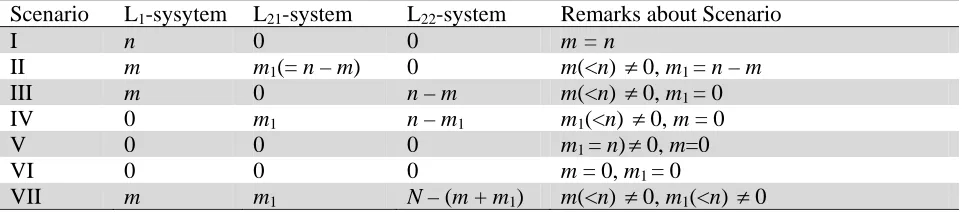
Table 1

Number of cycles of different system of different scenarios

Scenario L1-sysytem L21-system L22-system Remarks about Scenario

I n 0 0 m = n

II m m1(= n – m) 0 m(<n) ≠0, m1 = n – m

III m 0 n – m m(<n) ≠0, m1 = 0

IV 0 m1 n – m1 m1(<n) ≠0, m = 0

V 0 0 0 m1 = n)≠0, m=0

VI 0 0 0 m = 0, m1 = 0

VII m m1 N – (m + m1) m(<n) ≠0, m1(<n) ≠0

For the i-th (i∈NL1) cycle of L1- system, the differential Eq.s describing the inventory level are given by

1

1 1 ,0 ,2

( )

( ) ( ),

i

i i i

dq t

q t D t t t t

dt + θ = − ≤ ≤ (1)

1

,2 1,0 1,0

( ) ( )

,

1 ( )

i

i i

i

dq t D t

t t t

dt = − +δ t₊ −t < ≤ + (2)

with the boundary conditions

1 ,2, 1

1 1, ,0

( ) 0 at

( ) at

i i L

i L i i

q t t t i N

q t Q t t

= = ∈ _⎫⎪

⎬

= = _⎪⎭ (3)

The solutions of the differential Eq. (1) and (2) are as follows:

,2

1( ) exp( 1) ( ) exp( 1 ) , ,0 ,2

i

t

i i i

t

q t = − −θt

∫

D u θu du t ≤ ≤t t (4)

,2

1 ,2 1,0

1,0

( )

( ) ,

1 ( )

i

t

i i i

i t

D u

q t du t t t

t u

δ +

+

= < ≤

+ −

∫

(5)

The initial inventory level QL1,iof OW in i-th cycle is given by

,2

,0

1, 1( ,0) exp( 1 ,0) ( ) exp(1 )

i

t L i i i i

t

Q = q t = − θt

∫

D u θu du

= 1 , 2 , 0 2 , 2 2 , 0

1 1 1 1 1 1

ex p ( (i i ) ( ) i ( ) i

a b b a b b

t t t t

θ

θ θ θ θ θ θ

⎧ ⎫ ⎧ ⎫

⎪ ⎪ ⎪ ⎪

− ⎨ − + ⎬ ⎨− − + ⎬

⎪ ⎪ ⎪ ⎪

(7)

A. K. Bhunia et al. / International Journal of Industrial Engineering Computations 4 (2013) Now the inventory units deteriorated during the first cycle are given by

∫

= 2 , 0 , ) ( 1 1 , i i t t i i

OW q t dt

D θ Hence, 1 , 1 2 , 0 , ) ( θ i OW t t i D dt t q i i =

∫

i.e., the inventory carrying units during the i-th cycle is given by

= i OW q _, 1 , θ i OW D (7)

Again the deteriorated units during the i-th cycle is the difference between the initial inventory and the total selling

i.e.,

,2

,0

, 1, ( )

i

t OW i L i

t

D = Q −

∫

D t dt

{

}

2 2

1, ( ,2 ,0) ( ,2 ,0 )

2

L i i i i i

b

Q a t t t t

= − − − −

(8)

The total units backlogged quantities and the maximum level of shortages for i-th cycle is given by

1,0

,2

1,0 2

, 1( ) ( 1,0 ,2) 2 ( 1 1,0) log 1 ( 1,0 ,2)

2 i

i

t

i

L i i i i i i i

t

b t

b a

SQ q t dt t t t t t

b δ _δ _δ δ δ + + + + + = −

_∫

= − − + + + + − 1,0

1,0 1,0 ,2 1,0 ,2

2

1

( 1 i ) ( i i ) i log 1 ( i i )

t b a

t t t t t

b δ δ _δ _δ δ δ + + + + + ⎧ ⎫ + + + ⎨ − − + − ⎬ ⎩ ⎭ (9) and

BL,i=

1,0

,2

1 1,0 1,0 ,2 2 1,0 1,0 ,2

1,0

( )

( ) ( ) ( 1 ) log 1 ( )

1 ( )

i

t

i i i i i i i

i t

D t dt b b a

q t t t t t t

t t b

δ _δ _δ δ δ δ + + + + + + − = = − − + + + + − + −

∫

₍₁₀₎

Again, according to the earlier assumption, the i-th replenishment time t_i₊₁_,₀ can be expressed as

0 , 1

+

i

t = iT −i i( −1)γ / 2 ,i =0,1, 2, ...,n ₍₁₁₎

The length of the i-th cycle is t_i₊₁_,₀-t_i_,₀=T−( i−1) γ ₍₁₂₎

As the sum of the length of n replenishment cycle is H,

∑

= = − − n i H i T 1 ] ) 1 ( [ γ

which implies that

( 1) 2 H T n n γ = + − (13)

Again, for j-th (j∈NL21) cycle of L21-system, the differential Eq. governing the inventory system are

(8)

2

2 2 ,0 ,1

( )

( ) ( ),

j

j j j

dq t

q t D t t t t

dt + θ = − ≤ ≤ (14)

1

1 1 ,0 ,1

( )

( ) 0,

j

j j j

dq t

q t t t t

dt + θ = ≤ ≤ (15)

1

1 1 ,1 ,2

( )

( ) ( ),

j

j j j

dq t

q t D t t t t

dt + θ = − < ≤ (16)

( )

(

)

1

, 2 1,0 1,0 , 1 j j j j

dq t D t

t t t

dt = +δ t ₊ −t < ≤ + (17)

2( ,1) 0, 1( ,2) 0 , 1( ,0) 1

j j j j j j

q t = q t = q t = W ₍₁₈₎

Also, qj1(t) is continuous at t = tj,1. The solutions of the differential Eq. (14)-(17) using the boundary

conditions (18) are as follows

,1

2( ) ( ) exp{ (2 )} , ,0 ,1

j

t

j j j

t

q t = −

∫

D u θ u t du− t ≤ ≤t t (19)

1( ) 1 exp{ (1 ,0 )}, ,0 ,1

j j j j

q t = W θ t −t t ≤ ≤t t ₍₂₀₎

,2

1( ) exp( 1) ( ) exp( 1 ) , ,1 ,2

j

t

j j j

t

q t = − θt

∫

D u θu du t < ≤t t (21)

,2

1 , 2 1,0

1,0

( )

( ) ,

1 ( )

j

t

j j j

j t

D u

q t du t t t

t u

δ +

+

= < ≤

+ −

∫

(22)

Now the initial inventory level QL2,j of OW and RW in the j-th cycle (using (19)) is given by

QL2,j = W1 + qj2( tj,0 )= 1 2 ,1 ,0 2 ,1 2 ,0

2 2 2 2 2 2

exp( (j j )) ( ) j ( ) j

a b b a b b

W θ t t t t

θ θ θ θ θ θ

⎧ ⎫ ⎧ ⎫

+ − _⎨ − + _{⎬ ⎨}− − + _⎬

⎩ ⎭ ⎩ ⎭ (23)

Again, the inventory deteriorated during the j-th cycle in RW and OW are respectively given by

∫

− − = 1 , 0 , ) ( 1 , 2 , j j t t j L j

rw Q W D u du

D = 2 2

2, 1 { ( ,1 ,0) ( ,1 ,0 )}

2

L j j j j j

b

Q −W − a t −t + t −t ₍₂₄₎

and

∫

− = 2 , 1 , ) ( 1 , j j t t j

ow W D u du

D = 1 { ( ,2 ,1) ( ,22 ,12)} 2

j j j j

b

W− a t −t + t −t

(25)

Similarly, D_ow_,_j =θ₁QT_ow_,_j which implies that the inventory carrying units for j-th cycle in RW and OW are given by

, , / 2

rw j rw j

QT =D θ ₍₂₆₎

, , / 1

ow j ow j

QT =D θ ₍₂₇₎

Hence the expression for SQL,j and BL,j be the same as in (9) and (10) on substitution for i by j. Again

from the continuity of qj1(t) at t = tj,1, we have [from (20) and (21)]

,1

,2

1 ,1 1 1 ,0 ,1

( ) exp( ( )) exp( ( )

j

t

j j j

t

D u θ u−t du=W θ t −t

∫

(9)

A. K. Bhunia et al. / International Journal of Industrial Engineering Computations 4 (2013) 2

1 ,2 ,1 1 1 ,2 1 1 ,1 1 1 ,1 ,0

exp{ (θ tj −tj )}(aθ +b tθ j − −b) (aθ +b tθ j − =b) θ exp{−θ (tj −tj )} (28)

From the above Eq., it is not possible to find out the explicit form of tj,1 in terms of tj,2. Generally, the

value of θ1is quite small as it is the deterioration rate of items stored in OW. Thus, θ1(tj,2 – tj,1)<<1 and

1

θ (tj,1 – tj,0)<<1. Hence the series expansion of the exponential functions and ignoring the third and

higher degree terms, Eq. (28) reduces to

A1 tj,12 – B1tj,1 + C1 = 0 (29)

where

2

1 1 1j,2 1 1

A =aθ +b tθ − −b θ W (30)

1 2{ 1( j,2)j,2 1 1(1 1 j,0)}

B = a+θ a bt+ t −θW +θt ₍₃₁₎

2 2 2

1 j,2{2 ( 1 ) j,2 1 j,2} 1(2 2 1 j,0 1 j,0 )

C =t a+ aθ +b t +b tθ −W + θt +θ t (32)

Hence the Eq. (29) gives only the admissible solution 2

1 1 1 1

,1

1

4

2

j

B B A C

t

A

− −

= (33)

provided 2

1 4 1 1 0

B − A C >

Again, for the r-th (r∈NL22) cycle of L22-system, the differential Eq. describing the inventory level are

given by

2

2 2 ,0 ,1

( )

( ) ( ),

r

r r r

dq t

q t D t t t t

dt + θ = − ≤ ≤ (34)

1

1 1 ,0 ,1

( )

( ) 0,

r

r r r

dq t

q t t t t

dt + θ = ≤ ≤ (35)

1

1 1 ,1 ,2

( )

( ) ( ),

r

r r r

dq t

q t D t t t t

dt + θ = − < ≤ (36)

( )

(

)

1

, 2 1,0 1,0 , 1 r r r r

dq t D t

t t t

dt = +δ t₊ −t < ≤ + (37)

2( ,0) 2, 2( ,1) 0 , 1( ,0) 1, 1( ,2) 0

r r r r r r r r

q t =W q t = q t =W q t = ₍₃₈₎

The solutions of the differential Eq. (34)-(37) using the boundary conditions (38) are as follows

,1

2( ) ( ) exp( 2( )) , ,0 ,1

r

t

r r r

t

q t = −

∫

D u θ u t du− t ≤ ≤t t (39)

1( ) 1 exp{ (1 ,0 )}, ,0 ,1

r r r r

q t = W θ t −t t ≤ ≤t t ₍₄₀₎

,2

1( ) exp( 1) ( ) exp( 1 ) , ,1 ,2

r

t

r r r

t

q t = − θt

∫

D u θu du t < ≤t t (41)

,2

1 ,2 1,0

1,0

( )

( ) ,

1 ( )

r

t

r r r

r t

D u

q t du t t t

t u

δ +

+

= < ≤

+ −

∫

(42)

Now using the boundary condition qr2(tr, 0) = W2 implies that

2 ,1 ,0 2 ,1 2 ,0 2

2 2 2 2 2 2

exp( (r r ) ( ) r ( ) r

a b b a b b

t t t t W

θ θ θ θ θ θ θ ⎧ ⎫ ⎧ ⎫ ⎪ ⎪ ⎪ ⎪ − _⎨ − + _{⎬ ⎨}− − + _⎬= ⎪ ⎪ ⎪ ⎪ ⎩ ⎭ ⎩ ⎭ i.e., 2

2 2 ,0 2 2 2 ,1 ,0 2 2 ,1

(aθ +b tθ r − +b θ W) exp{−θ (tr −tr )}=aθ +b tθ r −b (43)

Like Eq. (28), Eq. (43) reduces to

(10)

A2tr,12 –B2tr,1 + C2 = 0

where

2

2 2 2r,0 2 2

A =aθ +b tθ − −b θ W (45)

2 2 2{( 2 2)(1 2r,0) 2r,0 }

B = a+θW +θ t +b tθ (46)

2 2 2 3

2 2(2 2 r,0 2 2r,0) 2 r,0 ( 2)r,0 2r,0

C =W +θ t + θt + at + +b aθ t +b tθ (47)

Hence the Eq. (44) gives only the admissible solution

2

2 2 2 2

,1

2

4 2

r

B B A C

t

A

− −

= (48)

provided 2

2 4 2 2 0

B − A C >

Again, from the continuity of qr1(t) at t = tr,1, we have from (40) and (41)

,1

,2

1 ,1 1 1 ,0 ,1

( ) exp( ( )) exp( ( ))

r

t

r r r

t

D u θ u−t du = W θ t −t

∫

which implies

1 1 ,0 ,1 1 ,2 ,1 2 ,2 2 ,1

1 1 1 1 1 1

exp{ (r r )} exp{ (r r )}[( ) r ] [( ) r ]

a b b a b b

W θ t t θ t t t t

θ θ θ θ θ θ

− = − − + − − + ₍₄₉₎

After simplification, then expanding the exponential functions and ignoring third and higher order terms of tr,2, Eq. (49) reduces to a quadratic Eq. in tr,2 as follows

A3 tr,22 – B3tr,2 + C3 = 0 (50)

where

2

3 1 1r,1 1 1

A =aθ +b tθ − +b θ W (51)

2

3 2{ (1 1r,1) 1r,1 1 1(1 1r,0)}

B = a+ +θt +b tθ +θW +θt (52)

2 2 2 3

3 1(2 2 1r,0 1 r,0 ) 2 1r,1 ( 1 )r,1 1r,1

C =W + θt +θ t + θt + aθ +b t +b tθ (53)

Hence the Eq. (50) gives only the admissible solution 2

3 3 3 3

,2

3

4 2

r

B B A C

t

A

− −

= (54)

provided 2

3 4 3 3 0

B − A C >

The other expressions of Drw,r, Dow,r, SQL,r, BL,r, QL2,r, QTrw,r, QTow,r can be derived similarly like L21

-sysytem. Now, the net profit (Z) for the entire planning horizon is given by

Z = <Sales revenue> - <purchase cost> - <carrying cost in OW and RW> - <backordering cost and penalty cost> -<ordering cost> - <transporting cost>

= 1 1, 2 2, 1 ,

1 1 1

( ) ( ( )

m n n

d r L i d r t L j d r L i

i j m i

P C C Q P C C C Q P C C B

= = + =

− −

∑

+ − − −

∑

+ − −

∑

, , , 1 2 1

1 1 1

1 2

( ) ( ) ( ) ( )

n n n

ow rw

ow i t rw j s L i l r r t

i j m i

C C

P D P C D C SQ nC n m W C C C

θ = θ = + =

− +

∑

− + −

∑

−

∑

− + − − + (55)

The above profit function Z is a function of three variables n, K1 and

γ

of which n is discrete and

γ

, K1

are continuous variables. We denote this as Z(n, γ, K1). Our objective is to determine the optimal values

(11)

A. K. Bhunia et al. / International Journal of Industrial Engineering Computations 4 (2013) Hence our problem is

1

max Z n( , γ, K)

1

subject to 0<γ,K ≤1 and n is an integer (56)

For a particular n, the corresponding m and m1 can be determined before the calculation of net profit

for the entire planning horizon. The values of m (number of cycles under L1-system) and m1(number of

cycles under L21-system) can be obtained from the following: m = max{j: qj1(tj,0) ≤W1}, j∈NL1

and m1= max{j-m: qj2(tj,0) ≤W2}, j∈NL21 (57)

The problem (56) can be solved by any classical method (gradient or direct search method) or by an well known soft computing method like Genetic Algorithm. As the gradient method or direct search method does not stuck to the global optimum, so we shall solve the problem by Genetic Algorithm. For this purpose, we shall develop an algorithm for determining the optimal values of m, m1, n, γ and K1

with the net profit of the proposed inventory system by a real-coded Genetic Algorithm (RCGA) for two different types of variables( discrete and continuous). The stepwise procedure of RCGA is shown in Algorithm -1,

Algorithm -1

Step-1: Initialize the parameters of RCGA, bounds of variables and different parameters of the proposed model.

Step-2: t = 0 [t represents the number of current generation].

Step-3: Initialize P(t) [P(t) represents the population with real coding of genes at t-th generation]. Step-4: Evaluate the fitness function of P(t).

Step-5: Find best found result from P(t). Step-6: t = t + 1

Step-7: If(t> maximum generation number) go to Step-14.

Step-8: Select P(t) from P(t – 1) by any selection process ranking selection. Step-9: Alter P(t) by crossover and mutation operations.

Step-10: Evaluate the fitness function of P(t). Step-11: Find the best found result from P(t).

Step-12: Compare the best found results of P(t) and P(t – 1) and store better one. Step-13: Go to Step-6.

Step-14: Print the best found result. Step-15: Stop.

To implement the above GA for the proposed model, the following basic components are considered.

• Parameters of GA.

• Chromosome representation.

• Initialization.

• Evaluation function.

• Selection process.

• Genetic operators(crossover and mutation)

3.1 Parameters of GA

(12)

of GA. However, there arise some difficulties in storing the data, if the population is too large. But if it is so small, there may not be enough populations for good crossovers.

3.2 Chromosome representation and Initialization

A main problem in applying a GA is to design an appropriate chromosome representation of solutions of the problem with genetic operations. Generally, traditional binary coding are used to represent the chromosome. This is not effective in many physical non-linear problems. As our proposed model is non-linear containing two different types of variables (discrete and continuous), a real number representation is used here. A real row matrix Vj = [Vj1,Vj2, Vj3] is used to represent a chromosome

where Vj1, Vj2 and Vj3 represent n ,

γ

and K1 respectively.

3.3 Initialization

After representation of chromosomes, the next step is to initialize the chromosomes that will take part in artificial genetics. In this process, first of all we have to find the independent variables and their bounds for the given problem. Then GA, POPSIZE number of chromosomes V1, V2, …,VPOPSIZE are

generated randomly, where every component for each chromosome is randomly generated within the boundary of the component. This set of chromosomes is taken as initial population.

3.4 Evaluation function

After getting a population of potential solutions, we need to see how good they are. Therefore, we have to calculate the fitness for each chromosome. In our problem, the value of the profit function for chromosome Vj (j =1,2, …, POPSIZE) is taken as the fitness of Vjand it is denoted by eval (Vj).In the

above mentioned algorithm, evaluation of P(t) in Step-4 and Step-10 in Algorithm – 1 is done by

function subprogram. In this function subprogram, generally population size numbers of objective function values are computed corresponding to the initialized values of independent variables. For different problems, this function subprogram is written differently. For our problem, the objective function values along with

γ

, K1, m (number of cycles under L1-system) and m1(number of cycles

under L21-system) will be computed in the function subprogram. The corresponding algorithm for

determining the optimal values of

γ

, K1, m and m1 along with objective function value for a particular

values of n and K1 is as follows:

Algorithm – 2

Step-1: Set i = 1, Z = 0 [Z stands for net profit of the system] Step-2: Compute ti,0 and ti,2.

Step-3: Compute qi1(ti,0)

Step-4: If qi1(ti,0) >W1, go to Step-8.

Step-5: Compute the profit Zi for the i-th cycle.

Step-6: Z = Z + Zi.

Step-7: i = i + 1 and go to Step-2. Step-8: m = i – 1.

Step-9: Set j = m + 1.

Step-10: Compute tj,0, tj,1 and tj,2.

Step-11: Compute qj2(tj,0).

Step-12: If qj2(tj,0) ≥W2, go to Step-15.

Step-13: Compute profit Zj, BL,j for j-th cycle.

Step-14: Z = Z + Zj, j = j + 1 and go to Step-9.

(13)

A. K. Bhunia et al. / International Journal of Industrial Engineering Computations 4 (2013) Step-16: Set k = m1 + m + 1.

Step-17: Compute tk,0, tk,1 and tk,2.

Step-18: Compute the profit Zk for the k-th cycle.

Step-19: Z = Z + Zk.

Step-20: k = k + 1.

Step-21: If (k≤n) go to Step-16. Step-22: Stop.

3.5 Selection Process

Here, the selection process is based on the ranking selection where the population is sorted from the best to the worst with selection probability assigned to of each individual according to their ranking. The process is explained precisely in the algorithm given below.

Step-1: Calculate the fitness fi, (i= 1,2, …, POPSIZE)

Step-2: Sort all fi’s in decreasing order for maximization problem and increasing order for minimization

problem.

Step-3: Generate a random number c∈[0,1].

Step-4: Calculate the probability pi of selection for each chromosome Vi by pi = c

(

)

1

1−c i−

Step-5: Compute the cumulative probability q_ifor each chromosome v_i using 1

i i j

j

q p

=

∑

Step-6: Generate another random real number d in [0,1].

Step-7: Obtain the minimal k such that qi >d and select the k-th interval.

Step-8: Repeat Step-6 and Step-7 until the number of selected individuals becomes population size.

3.6 Crossover Operation

After the selection process, other genetic operators, like crossover and mutation are applied to the resulting chromosomes i.e., those which have survived. Crossover is an operator that creates new individuals/ chromosomes (offspring) by recombining the features of both parent solutions. It operates on two or more parent solutions at a time and produces offspring for the next generation. In this operation, expected N (the integral value of PCROS*POPSIZE) numbers of chromosome will take part. Hence, in order to perform the crossover operation, select N numbers of chromosome. After selection of chromosomes, the whole arithmetic crossover is applied here. In our problem, each chromosome Vi

has three genes Vi1, Vi2 and Vi3, of which first one is discrete and other two are continuous variables.

Different steps of crossover operation is given below:

Step-1: Find the integral value of PCROS*POPSIZE and store it in N.

Step-2: Select two chromosomes Vj and Vk randomly from the population for crossover

Step-3: Generate a proper fraction λ by the formula

λ = pmax / (pmax + pmin)

where pmax = max[ pi, i =1,2, …, POPSIZE]

and pmin = min[ pi, i =1,2, …, POPSIZE]

Step-4: Compute the components Vjl ′ and Vkl′ of two offspring Vj′and Vk ′ by

Vjl/ = λVjl + (1- λ) Vkl Vkl/ = λVkl + (1- λ) Vjl

Step-5: Compute the components Vj′1 and Vk′1 of two offspring by either V′ =j1 Vj1+g and Vk′ =1 Vk1−g if

1 1

j k

V <V or Vk′ =1 Vk1+g and Vj′ =1 Vj1−g where g is a random integer number between 0 and

1 1

j k

V −V .

(14)

3.7 Mutation Operation

This operation is responsible for fine-tuning capabilities of the system. It is applied to a single chromosome. Here, we shall use uniform and non-uniform mutation for discrete and continuous variables respectively. The action of non-uniform mutation depends on the age of the population. If the element Vik of Vi chromosome is selected for this mutation and domain of Vik is [lk, uk], then the reduced

value of Vik is given by

( , ), 0.5

( , ),

ik k ik ik

ik ik k

V t u V when r V

V t V l othere wise

+ Δ − ≤

⎧

′ = ⎨ _{− Δ} ₋

⎩

where k∈[1,2,3], Δ (t,y) returns a value in the range [0,y] and r is a uniformly distributed random number in [0,1].

In our study, we have taken

Δ (t, y) = a random integer between [0,y] for discrete variable.

=

b

1

yr 1- t

T

⎛ ⎞

⎜ ⎟

⎝ ⎠ , for a continuous variable.

where r₁is a uniformly distributed random number in [0,1] , t, T and b represent the current generation,

MAXGEN and the constant respectively.

3.8 Ellitism

As GA technique is a stochastic optimization technique, sometimes, the best chromosome may be lost when a new population is created by crossover and mutation. To overcome this situation the worst individual/chromosome of the current generation is replaced by the best individual/chromosome of previous generation. Instead of single chromosome one or more chromosomes may take part in this operation. This is called elitism.

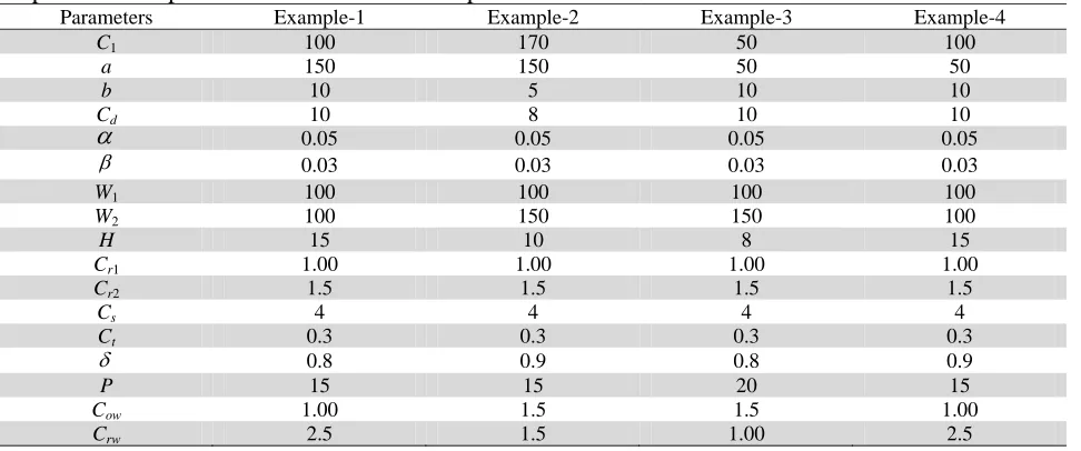
4. Numerical Examples

To illustrate the developed model, four examples have been considered. The values of different parameters are given in the Table 2. For these numerical examples, the model parameters values have not been collected from any case study, but these values considered here are realistic.

Table 2

Input values of parameters for different examples

Parameters Example-1 Example-2 Example-3 Example-4

C1 100 170 50 100

a 150 150 50 50

b 10 5 10 10

Cd 10 8 10 10

α

0.05 0.05 0.05 0.05

β 0.03 0.03 0.03 0.03

W1 100 100 100 100

W2 100 150 150 100

H 15 10 8 15

Cr1 1.00 1.00 1.00 1.00

Cr2 1.5 1.5 1.5 1.5

Cs 4 4 4 4

Ct 0.3 0.3 0.3 0.3

δ 0.8 0.9 0.8 0.9

P 15 15 20 15

Cow 1.00 1.5 1.5 1.00

(15)

This RCGA has been coded in C Programming language. The computational work has been done an a PC with Intel Core-2-duo 2.5 GHz Processor in LINUX environment. Solving the non-linear constrained optimization problem (55) by RCGA method, the optimum values of m, m1, γ, K1, n and

the corresponding profits for all examples have been obtained. The computational results have been shown in Table 3.

Table 3

Optimal results for different examples

Example-1 Example-2 Example-3 Example-4 No. of cycles under L1

-system (m) 7 0 10 10

No. of cycles under L21

-system (m1)

20 12 0 6

No. of cycles under L22

-system (n-m-m1) 0 0 0 0

Optimal no. of cycles 27 12 10 16

K1 0.6968325 0.6952205 0.8394946 0.7462106

γ 0..218582 0.0181895 0.2984824 0.0360834

Profit (Z) ( in $) 9699.21 7188.60 5478.35 4772.47

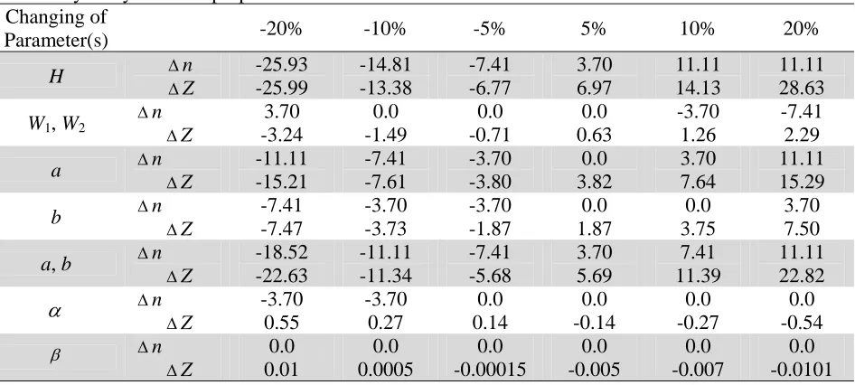
5. Sensitivity Analysis

Using the numerical Example-1 mentioned earlier, the effect of under or over estimation of various

parameters on replenishment policy and maximum net profit is studied. Here, we employ,

Δn = (n/ - n)/n× 100%, ΔZ = (Z/ - Z)/ Z× 100% as measure of sensitivity, where n and Z are the true values and n/, Z/ the estimated values. The sensitivity analyses are shown by increasing or decreasing the parameters by 5%, 10% and 20%, taking one or more at a time and keeping the others at their true values. The results are presented in Table 4, which are self-explanatory.

Table 4

Sensitivity analysis of the proposed model Changing of

Parameter(s) -20% -10% -5% 5% 10% 20%

H Δn

ΔZ -25.93 -25.99 -14.81 -13.38 -7.41 -6.77 3.70 6.97 11.11 14.13 11.11 28.63

W1, W2

Δn ΔZ 3.70 -3.24 0.0 -1.49 0.0 -0.71 0.0 0.63 -3.70 1.26 -7.41 2.29

a Δn ΔZ -11.11 -15.21 -7.41 -7.61 -3.70 -3.80 0.0 3.82 3.70 7.64 11.11 15.29

b Δn ΔZ -7.41 -7.47 -3.70 -3.73 -3.70 -1.87 0.0 1.87 0.0 3.75 3.70 7.50

a, b Δn ΔZ -18.52 -22.63 -11.11 -11.34 -7.41 -5.68 3.70 5.69 7.41 11.39 11.11 22.82

α

Δn

ΔZ -3.70 0.55 -3.70 0.27 0.0 0.14 0.0 -0.14 0.0 -0.27 0.0 -0.54

β Δn

(16)

5. Concluding Remark

In the present day competitive marketing situation, when the area of existing warehouse (Owned warehouse, OW) in an important market place (like, super market, corporation market, etc.) is relatively small, then the inventory management authority is bounded to hire a separate warehouse on rental basis. Considering this situation, we have developed a deterministic inventory model for deteriorating items over a finite time horizon. In the model formulation, we have also removed the unrealistic assumption regarding the storage capacity of rental warehouse in the existing models developed by Hartely (1976), Sarma (1983), Dave (1988) and Bhunia and Maiti (1994) and others. The replenishment cost is taken to be dependent on the lot size of the current replenishment. This model is applicable for foodgrains like paddy, wheat, rice, etc., as the demand of the foodgrains increases with time for a fixed time horizon i.e., for a calendar year. It is also applicable for other items whose demands increase linearly with time. On the other hand, the case of decreasing demand is also of great importance for a finite horizon model. The results available in this work are also valid for linearly decreasing demand. For further research, one can extend the model developed in this paper for multiple items, quantity discount policies and imprecise demand.

References

Benkherouf, L A., (1997). A deterministic order level inventory model for deteriorating items with two storage facilities. International Journal of Production Economics, 48, 167-175.

Bhunia, A. K.,& Maiti, M. (1994). A two-warehouse inventory model for a linear trend in demand.

Opserach, 31, 318-329.

Bhunia, A. K.,& Maiti, M. (1997). A two warehouses inventory model for deteriorating items with linear trend in demand and shortages. Journal of Operational Research Society, 49, 287-292. Bhunia, A.K.,& Maiti, M. (1999). An inventory model of deteriorating items with lot-size dependent

replenishment cost and a linear trend in demand. Applied Mathematical Modeling, 23, 302-308. Bhunia, A.K., Pal, P., Chattopadhyay,S.,& Medya, B. K. (2011) An inventory model of

two-warehouse systemwith variable demand dependent on instantaneous displayed stock and marketing decisions via hybrid RCGA. International Journal of Industrial Engineering Computations, 2, 351– 368.

Chakrabarti, T.,& Chaudhuri, K S. (1997). An EOQ model for deteriorating items with a linear trend I demand and shortages in all cycles. International Journal of Production Economics, 49, 205-213. Chung, K J.,& Ting, P. S. (1993). A heuristic for replenishment of determining items with a linear

trend in demand. Journal of Operational Research Society, 44, 1235-1241.

Chung, K.J., & Huang, T.S. (2007). The optimal retailer’s ordering policies for deteriorating items with

limited storage capacity under trade credit financing. International Journal of Production

Economics, 106, 127-145.

Das, B., Maity,K., & Maiti, M. (2007).A two warehouse supply chain model under possibility/necessity/credibility measures. Mathematical and Computer Modeling, 46, 398-409. Datta, T. K.,& Pal, A. K. (1992). A note on a replenishment policy for an inventory model with linear

trend in demand and shortages.Journal of Operational Research Society, 43, 993-1001.

Dave, U. (1989). A deterministic lot-size inventory model with shortages and a linear trend in demand,

Naval Research Logistics, 36, 507-514.

Dave, U. (1998). On the EOQ models with two levels of storage.Opsearch, 25, 190-196.

Dey, J.K., Mondal, S.K., & Maiti, M. (2008).Two storage inventory problem with dynamic demand and interval valued lead-time over finite time horizon under inflation and time-value of money.

European Journal of Operational Research, 185, 170-194.

Donaldson, W. A. (1977). Inventory replenishment policy for a linear trend in demand-an analytical solution. Operation Research Quarterly, 28, 663-670.

Goldberg, D. E. (1989).Genetic Algorithms: Search Optimization and Machine Learning. Addison

(17)

Goswami, A.,& Chaudhuri, K. S. (1992). An economic order quantity model for items with two levels of storage for a linear trend in demand. Journal of Operational Research Society, 43, 157-167. Goyal, S. K., Horiga, M. A.,& Alyan, A. (1996). The trended inventory lot sizing problem with

shortages under a new replenishment policy. Journal of Operational Research Society, 47, 1286-1295.

Goyal, S. K., Morin, D.,& Nebebe, F. (1992). The finite horizon trend inventory replenishment problem with shortages. Journal of Operational Research Society, 43, 1173-1178.

Hartely, R. V. (1976). Operations Research-a managerial emphasis. Goodyear publishing Company,

315-317.

Horiga, M. (1994). The inventory lot-sizing problem with continuous time-varying demand shortages.

Journal of Operational Research Society, 45, 827-837.

Hsieh, T.P., Dye, C.Y., & Ouyang, L.Y. (2008). Determining optimal lot size for a two-warehouse system with deteriorating and shortages using net present value. European Journal of Operational Research, 191, 180-190.

Jaggi, C.K., Aggarwal, K.K., & Goel, S.K. (2006). Optimal order policy for deteriorating items with inflation induced demand. International Journal of Production Economics, 34, 151-155.

Jaggi, C.K., Khanna, A., & Verma, P. (2011).Two-warehouse partial backlogging inventory for

deteriorating items with linear trends in demand under inflationary conditions. International

Journal of Systems Science, 42(7), 1185-1196.

Kar, S., Bhunia , A. K.,& Maiti, M. (2001) Deterministic inventory model with two levels of storage, a linear trend in demand and a fixed time horizon. Computers and Operations Research, 28, 1315-1331.

Khouja, M., Michalawicz, Z.,& Wilmot, M. (1998) The use of Genetic Algorithms to solve the economic lot-size scheduling problem. European Journal of Operational Research, 110, 509-524. Lee, C. C.,& Ma, C. Y. (2000) Optimal inventory policy for deteriorating items with two warehouse

and time dependent demands. Production Planning And Control, 7, 689-696.

Lee, C.C. (2006). Two-warehouse inventory model with deterioration under FIFO dispatching policy.

European Journal of Operational Research, 174, 861-873.

Mandal, S.,& Maiti, M., (2002). Multi-item fuzzy EOQ models using genetic algorithm.Computers and Industrial Engineering, 44, 105-117.

Michalawicz, Z. (1996).Genetic Algorithms + Data Structures=Evoluation Programs. Springer Verlog,

Berlin.

Mitra, A., Cox, J. F.,& Jesse, R. R. (1984). A note on determining order quantities with linear trend in demand. Journal of Operational Research Society, 35, 439-442.

Niu, B., & Xie, J. (2008). A note on two-warehouse inventory model with deterioration under FIFO dispatch policy. European Journal of Operational Research, 190, 571-577.

Pakkala, T. P. M.,& Achary, K. K. (1992). A deterministic inventory model for deteriorating items with two warehouses and finite replenishment rate. European Journal of Operational Research, 57, 71-76.

Pal, P., Das, C. B., Panda, A.,& Bhunia, A. K. (2004). An application of Read-coded Genetic Algorithm (For mixed integer non-linear programming in an optimal two-warehouse inventory policy for deteriorating items with a linear trend in demand and fixed planning horizon).

International Journal of Computer Mathematics, 82(2), 163-175.

Rong, M., Mahapatra, N.K., & Maiti, M. (2008). A two warehouse inventory model for a deteriorating

items with partially/fully backlogged shortage and fuzzy lead time. EuropeanJournal of

Operational Research, 189, 59-75.

Ritchie, E. (1984). The EOQ for linear increasing demand: a simple optimal solution. Journal of

Operational Research Society, 35, 949-952.

Sakawa, M. (2002).Genetic Algorithms and fuzzy multi-objective optimization. Kluwer Academic

Publishers.

(18)

Sarma, K. V. S. (1983). A deterministic inventory model with two levels of storage and an optimum release rule. Opsearch, 29, 175-180.

Sarma, K. V. S. (1987). A deterministic order-level inventory model for deteriorating items with two storage facilities. European Journal of Operational Research, 29, 70-72.

Silver, E. A.,& Meal, H. C., (1973). A heuristic for selecting lot-size quantities for the case of a deterministic time varying demand rate and discrete opportunities for replenishment. Production Inventory Management, 14, 64-74.

Silver, E. A. (1979). A simple inventory decision rule for a linear trend in demand, Journal of

Operational Research Society, 30, 71-75.

Stanfel, L. E., & Sivazlian, B. D. (1975).Analysis of system in operations. Englewood Cliffs, NJ: Prentice-Hall.

Yang, H.L., Teng, J.T., & Chern, M.S. (2001). Deterministic inventory lot-size models under inflation with shortages and deterioration for fluctuating demand. Naval Research Logistics, 48, 144-158. Yang, H.L. (2004). Two-warehouse inventory models for deteriorating items with shortage under

inflation. European Journal of Operational Research,157, 344-356.