Clustering fuzzy objects using ant colony optimization Pages 115-126 Download PDF

* Corresponding author. Tel./fax: +98-871-6660073 E-mail: [email protected] (F. Ahmadizar) © 2014 Growing Science Ltd. All rights reserved. doi: 10.5267/j.ijiec.2013.09.003

International Journal of Industrial Engineering Computations 5 (2014) 115–126

Contents lists available at GrowingScience

International Journal of Industrial Engineering Computations

homepage: www.GrowingScience.com/ijiec

Clustering fuzzy objects using ant colony optimization

Fardin Ahmadizara* and Mehdi Hosseinabadi Farahanib

a

Department of Industrial Engineering, University of Kurdistan, Pasdaran Boulevard, Sanandaj, Iran b

Department of Industrial Engineering, College of Engineering, University of Tehran, Tehran, Iran C H R O N I C L E A B S T R A C T

Article history: Received June 2 2013

Received in revised format September 7 2013

Accepted September 7 2013 Available online September 9 2013

This paper deals with the problem of grouping a set of objects into clusters. The objective is to minimize the sum of squared distances between objects and centroids. This problem is important because of its applications in different areas. In prior literature on this problem, attributes of objects have often been assumed to be crisp numbers. However, since in many realistic situations object attributes may be vague and should better be represented by fuzzy numbers, we are interested in the generalization of the minimum sum-of-squares clustering problem with the attributes being fuzzy numbers. Specifically, we consider the case where an object attribute is a triangular fuzzy number. The problem is first formulated as a fuzzy nonlinear binary integer programming problem based on a newly proposed dissimilarity measure, and then solved by developing and demonstrating a problem-specific ant colony optimization algorithm. The proposed algorithm is evaluated by computational experiments.

© 2013 Growing Science Ltd. All rights reserved

Keywords:

Clustering Fuzzy objects Dissimilarity measure Minimum sum-of-squares Ant colony optimization

1. Introduction

Clustering involves partitioning a set of objects into clusters in such a way that the objects belonging to the same cluster must be as similar as possible, while those belonging to different clusters must be as dissimilar as possible. Cluster analysis has found applications in different areas including image segmentation, information retrieval, marketing, analysis of chemical compounds, etc. Considering the crispness or fuzziness of classes as well as attributes of objects, clustering models can be categorized as follows (D’Urso & Giordani, 2006):

In crisp clustering, also known as hard clustering, each object would just belong to one cluster, while in fuzzy clustering an object has a degree of membership in each cluster, i.e., the clusters are allowed to overlap. In both crisp and fuzzy clustering, object attributes may be represented by crisp or fuzzy numbers.

Most of studies conducted on clustering problems have mainly assumed that object attributes are fixed and deterministic (crisp clustering of crisp objects, in particular). However, in many real-world situations, due to the imprecise or uncertainty of data sources, the attributes should better be represented by fuzzy numbers. Consequently, dealing with clustering of fuzzy objects can provide a great deal of applications and advantages.

The k-means algorithm (MacQueen, 1967) and its variations such as the global k-means algorithms (Likas et al., 2003; Bagirov, 2008) are the most popular crisp clustering methods. However, to obtain better clustering results, researchers have recently focused on the use of metaheuristic algorithms like genetic algorithms (Kivijarvi et al., 2003; Handl & Knowles, 2007; Chang et al., 2009; Xiao et al., 2010), tabu search (Al-Sultan, 1995; Liu et al., 2008), simulated annealing (Sun et al., 1994), ant colony optimization (ACO) algorithms (Shelokar et al., 2004; Runkler, 2005) and hybrid algorithms (Pirzadeh et al., 2012).

The fuzzy c-means algorithm (Bezdek, 1981) and its variations such as the Gustafson-Kessel algorithm (Gustafson & Kessel, 1979) are the most popular fuzzy clustering techniques. Metaheuristic algorithms have also been applied to solve fuzzy clustering problems (see, e.g., Al-sultan & Fedjki, 1997; Kanade & Hall, 2004). However, some researchers have paid attention to fuzzy data. Hathaway et al. (1996) have proposed fuzzy c-means clustering for trapezoidal fuzzy numbers. A fuzzy c-numbers clustering procedure for LR-type fuzzy numbers has been proposed by Yang and Ko (1996), and extended to conical fuzzy vectors by Yang and Liu (1999). Yang et al. (2004) have suggested fuzzy clustering algorithms for symbolic and fuzzy data. The so-called alternative fuzzy c-numbers clustering algorithm for LR-type fuzzy numbers has been proposed by Hung and Yang (2005) based on an exponential-type distance measure. D’Urso and Giordani (2006) have proposed a fuzzy c-means clustering model based on a weighted dissimilarity measure for comparing pairs of symmetric fuzzy data. Hung et al. (2010) have suggested a clustering procedure, which is robust to initials and cluster number, by modifying the similarity-based clustering method proposed by Yang and Wu (2004) to handle LR-type fuzzy numbers. Recently, Jafari et al. (2013) have investigated for clustering cellular manufacturing the performance of two fuzzy clustering methods.

This paper deals with the problem of crisp clustering of fuzzy objects. We consider the case where each object attribute is a triangular fuzzy number (TFN). In order to introduce a dissimilarity measure between fuzzy data, the (squared) Euclidean distance is generalized to TFNs. The problem is formulated as a fuzzy nonlinear binary integer programming problem with the objective of minimizing the sum of squared distances between objects and centroids. To solve the problem efficiently, an ant colony optimization algorithm is then proposed.

The rest of the paper is organized as follows. In the next section, the problem is introduced and formulated. The proposed ACO algorithm is described in Section 3, followed by Section 4 providing computational results. Finally, Section 5 concludes the paper.

2. Crisp clustering of fuzzy objects

2.1 Problem definition

Let w_ijbe the association weight variable of object i with cluster j, which can be assigned as 1, if object is allocated to cluster

, 1,..., , 1,..., 0, otherwise

ij

i j

w _ i  N j  K

 

Assuming that the objective is to minimize the sum of squared error, which is the most frequently used criterion in non-hierarchical (i.e., partitional) clustering (Jain et al., 1999), the problem of crisp clustering of fuzzy objects can be formulated as the following fuzzy nonlinear binary integer programming problem: 2 1 1 1 1 min

s.t. 1, 1,...,

1, 1,...,

{0,1}, 1, ..., , 1,...,

K N ij ij j i K ij j N ij i ij

Z w D

w i N

w j K

w i N j K

           

 





  (1)

where D_ij denotes a (fuzzy) distance between object i and the center of cluster j, due to the fact that

each cluster is identified by its center (or centroid). Clearly, each cluster center is an R-dimensional vector of fuzzy sets as well. It is noted that the first set of constraints ensures that each object belongs to only one cluster, while the second set of constraints ensures that at least one object is assigned to each cluster.

In the problem considered in this paper, it is assumed that TFNs are used to embody the imprecise and uncertainty of data sources. For a TFN, a particular case of fuzzy sets, the decision maker only needs to estimate three values for an object attribute: the most plausible, pessimistic and optimistic values. Let

il

A



be the TFN representing the value of the lth attribute of object i.

A



_il is denoted by triplet

1 2 3

(a_il, a_il, a_il), where a_il1 (most pessimistic value), a_il2 (most plausible value) and a_il3 (most optimistic value) are real numbers with 1 2 3

il il il

a a a . The membership function of

A



_il is then defined as (for real number x)

1 1 2 2 1 2 3 2 3 3 2 , 1,

( ) , 1,..., , 1,...,

,

0, otherwise il il il il il il il A il il il il il x a

a x a

a a

x a

x i N l R

a x

a x a

a a          _  _     _{ }  _    

The lth attribute value of the center of cluster j is denoted by M_jl, which can be obtained by averaging

the lth attribute values of all objects belonging to the cluster as follows:

1 1

, 1,..., , 1,...,

N ij il i jl N ij i w A

M j K l R

Since, as is well-known, the multiplication/division of a TFN by a scalar as well as the addition/subtraction of two or more TFNs becomes also a TFN (for more discussion on this type of fuzzy numbers, the reader is referred to Kaufmann & Gupta, 1991), M_jl is shown by triplet

1 2 3

(m_jl, m_jl, m_jl), where

1 1

, 1, 2,3, 1,..., , 1,...,

N q ij il

q i

jl N

ij i

w a

m q j K l R

w





   





(3)

As seen, like each of the objects, each cluster center is represented as an R-dimensional vector of TFNs.

2.2 Dissimilarity measure

This subsection describes how the distance between object i and the center of cluster j, i.e., D_ij given

in model (1), is measured. In the literature, several measures of distance, dissimilarity and similarity between fuzzy data have been suggested (see, e.g., Pappis & Karacapilidis, 1993; Bloch, 1999; Szmidt & Kacprzyk, 2000; Kim & Kim, 2004; Yong et al., 2004; D’Urso & Giordani, 2006). However, in order to measure the distance between a pair of multidimensional vectors of TFNs, the traditional Euclidean distance is utilized and adopted.

By generalizing the squared Euclidean distance to TFNs, 2 ij

D , referred to as the dissimilarity between

object i and the center of cluster j, can then be calculated as follows:

2 2

1

, 1,..., , 1, ...,

R

ij ijl

l

D d i N j K







  

 ₍₄₎

where

ijl il jl

d A M (5)

It is clear that d_ijl defined in Eq. (5) is a TFN as well. Therefore, d_ijl is denoted as (d_ijl1, d_ijl2, d_ijl3), where

3 ( 1)_{, 1, 2,3, 1,..., , 1,..., , 1,...,}

q q q

ijl il jl

d _a _m   q _ i _ N j _ K l _ R

(6)

Unfortunately however, since dijl2 on the basis of the extension principle does not become a TFN, for

simplicity, it is approximated as a TFN in the following way.

Definition 1 dijlis a positive TFN if 1

0

ijl

d  . It is a negative TFN if d_ijl3 0. It is neither positive nor negative if d_ijl1 0 and d_ijl3 0.

Definition 2 If d_ijl is positive, then

2 1 2 2 2 3 2

(( ) , ( ) , ( ) )

ijl ijl ijl ijl

d  d d d (7)

If d_ijl is negative, then

2 3 2 2 2 1 2

(( ) , ( ) , ( ) )

ijl ijl ijl ijl

d  d d d (8)

And in the case where d_ijl is neither positive nor negative, then

2 2 2 1 2 3 2

(0, ( ) , max(( ) , ( ) ))

ijl ijl ijl ijl

2.3 Some remarks

Theorem 1The proposed dissimilarity measure is a symmetric function.

Proof Taking into account Eqs. (4) and (5), to show that 2 ij

D is a symmetric function, it suffices to

show that

2 2

(A_il M _jl) (M _jlA_il) (10)

Let us consider the case where A_il M_jl is positive. Then, from Eq. (7),

2 1 3 2 2 2 2 3 1 2

(A_il M_jl) ((a_il m_jl) , (a_il m_jl) , (a_il m_jl) )

Since

1 3 2 2 3 1

(M _jlA_il)(m_jl a_il, m_jl a_il, m_jl a_il)

obviously, in this case M_jl  A_il is negative and then, from Eq. (8),

2 3 1 2 2 2 2 1 3 2

(M_jl A_il) ((m_jl a_il) , (m_jl a_il) , (m_jl a_il) )

As seen, Eq. (10) holds. In the case where A_il M _jl is negative, since M_jl A_il is positive, in a similar

way we can easily show Eq. (10) holds. Furthermore, if A_il M_jl is neither positive nor negative,

jl il

M A is neither positive nor negative as well. Then, from Eq. (9),

2 2 2 2 1 3 2 3 1 2

(

A



_il



M



_jl

)



(0, (

a

_il



m

_jl

) , max((

a

_il



m

_jl

) ,(

a

_il



m

_jl

) ))

and

2 2 2 2 1 3 2 3 1 2

(

M



_jl



A



_il

)



(0, (

m

_jl



a

_il

) , max((

m

_jl



a

_il

) ,(

m

_jl



a

_il

) ))

Again, Eq. (10) holds, and the proof is complete. ∎

Furthermore, from Definition 2 it follows that d_ijl2 is always approximated by a positive TFN. Taking into account Eq. (4), we then have the following corollaries.

Corollary 1The distance between a pair of multidimensional vectors of TFNs is measured by a TFN.

Corollary 2The proposed dissimilarity measure is positive (i.e., a positive TFN).

Theorem 1 and Corollary 2 show two essential properties of a distance measure. However, there is another important issue to be considered. When a cluster contains just one object, its centre clearly coincides with that object (this is also shown by Eq. (3)) and consequently, the distance between the object and the cluster center should be zero. In other words, such a cluster should not have any contribution to the objective function. Due to the fact that the subtraction of two equal TFNs does not become zero (see Eq. (5) and Eq. (6)), from Eq. (4), singleton clusters would therefore have an undesirable effect on the objective function if not revised. Hence, the objective function of model (1) is modified as follows:

2

1 1

,

K N

j ij ij

j i

Z y w D

 



_{ }

  ₍₁₁₎

1

1

1, 1

, 1,...,

0, 1

N ij i j N ij i w

y j K

w       _     





It is then easy to show that

1 1

1

2

min 1, 1 , 1,...,

2 N N ij ij N i i j ij i w w

y w   j K

      _  _   







(12)

Considering Eq. (11) and Eq. (12), the problem of crisp clustering of fuzzy objects can then be formulated as follows (without additional variables y_j):

1 1 2

1 1 1 1 2 min 2

s.t. 1, 1,...,

1, 1,...,

{0,1}, 1, ..., , 1,...,

N N Ij Ij K N I I ij ij j i K ij j N ij i ij w w

Z w D

w i N

w j K

w i N j K

               





 





  (13)

Since 2 ij

D is a TFN, the objective function of the above model is obviously the sum of some TFNs. We

then have the following corollary.

Corollary 3The objective function of model (13) becomes a TFN.

Theorem 2 The traditional minimum sum-of-squares clustering problem (with crisp object attributes)

is a particular case of the problem of crisp clustering of fuzzy objects stated in model (13).

Proof Consider the case where the uncertainty of data sources is neglected by the decision maker. In this situation, each object attribute is undoubtedly set equal to its most plausible value, that is, the value of the lth attribute of object i is set to 2

il

a . It is then easy to show, considering Eqs. (2–9), that the proposed dissimilarity measure is reduced to the traditional squared Euclidean distance and consequently, the problem stated in model (13) to the traditional minimum sum-of-squares clustering problem. In other words, the latter problem is a particular case of the former one. ∎

3. Proposed ant colony algorithm

To solve the problem under consideration, an ant colony algorithm is developed. ACO algorithms, firstly introduced by Dorigo (1992), are population-based, cooperative search procedures derived from the behavior of real ants. Without using visual cues, real ants exploiting pheromones as a communication medium are able to find the shortest path from the nest to a food source. After representing a combinatorial optimization problem by a graph, an ACO algorithm makes use of simple agents, called artificial ants, to move across the graph and iteratively construct solutions. That is, an artificial ant builds a complete solution by starting with a null one and iteratively adding solution components. Moreover, artificial ants deposit pheromones on their path, and the generation of solutions is then guided by the pheromone trails. ACO algorithms have thus far had substantial applications in many hard optimization problems, such as reliability optimization (Ahmadizar & Soltanpanah, 2011) and scheduling (Ahmadizar & Hosseini, 2012) problems. For further details on ACO algorithms, interested readers may refer to Dorigo & Stutzle (2004).

3.1 Solution construction

To apply an ACO algorithm to the problem of crisp clustering of fuzzy objects stated in model (13), it is represented by a graph with two types of nodes. The first set of nodes contains one element for each object and the other contains one element for each cluster. Each node in the first set is then connected to each node in the second set by an edge, indicating that each object can be assigned to each cluster. To construct a solution, an artificial ant starts from the first object and chooses (moves to) one of the clusters by applying a transition rule. In other words, the object is assigned to the chosen cluster. Then, the ant iteratively moves to the next object and chooses a cluster. Clearly, each ant may move to a node corresponding to a cluster several times.

Let



ij be the pheromone trail between object i and cluster j, i.e., the pheromone trail associated with

edge (i, j) of the given graph.



_ij shows the desirability of assigning object i to cluster j. The pheromone trails are regularly modified at run-time and form a kind of adaptive memory of previously found solutions. As mentioned, while constructing a solution, an object is assigned to a cluster by an ant according to a transition rule so-called pseudo-random proportional rule (Dorigo & Gambardella, 1997) as follows: with probability q0 an ant v for object i chooses the cluster j for which the pheromone

trail is maximum, that is, jarg max(



_ij). While with probability 1-q0, the ant chooses a cluster j

according to the probability distribution given in the following equation:

1

, 1,...,

ij v

ij K

ih h

p



j K





 



(14)

As seen, q0 (a parameter between 0 and 1) determines the relative importance of exploitation versus

exploration. Moreover, it is noteworthy that the heuristic information is not employed in the proposed approach. The heuristic information, unlike the pheromone trails, represents a priori information about the problem instance definition provided by a source different from the artificial ants. The reason is that by assigning an object to a cluster, the cluster centre given in Eq. (2) relocates frequently and hence, the heuristic information may not be introduced appropriately.

3.2 Repairing infeasible solutions

solution constructed by an ant, a straightforward procedure based on a neighborhood search is therefore developed in which the infeasible solution is always replaced by a feasible one as follows:

Step 1.Determine empty clusters.

Step 2.For each empty cluster j, do the following (in an increasing order of j):

2.1. Among objects that their cluster has at least two objects, randomly select one. 2.2. Reassign the selected object to cluster j.

3.3 Updating of the pheromone trails

In the beginning, each pheromone trail is set equal to a fixed value τ0=0.1 and then, at run-time, the

pheromone trails are regularly modified according to a global updating rule. This rule is proposed to increase the pheromone values compatible to better solutions to make the search more directed.

Once all ants have constructed their solutions (and after repairing infeasible solutions), each pheromone trail compatible to the solution generated by ant v (for each ant in the colony) is updated as follows:

(1 ) ,

ij ij

v z



     (15)

where ρ, a parameter between 0 and 1, is the pheromone trail evaporation rate and z_v is a defuzzified value of the objective function for the solution of ant v. Then, each pheromone trail compatible to the best solution obtained so far is updated as follows:

(1 ) ,

ij ij

best B

z



     (16)

where z_best is a defuzzified value of the objective function for the best solution obtained up to now and

B is a positive parameter determining the relative importance of this solution. It should be noted here that the value of the objective function for each (feasible) solution is defuzzified to not only apply the above updating rule but also compare a new generated solution with the best one generated so far. Several ranking methods for defuzzification/comparison of fuzzy sets are available in the literature (see, e.g., Chang & Lee, 1994; Chu & Tsao, 2002; Abbasbandy & Hajjari, 2009). In this study, however, the overall existence ranking index proposed by Chang and Lee (1994) is adopted to defuzzify Z, which is a TFN (as stated in Corollary 3) denoted by _{( , , )z}1 _z2 _z3 _{. The defuzzified value} (with the pure weighting; for more discussion on the various weightings, the reader is referred to Chang & Lee, 1994) is then defined as

1 2 3

( 4 )

6

z z z

z   (17)

3.4 General structure of the algorithm

In the following, the general structure of the ACO algorithm proposed to solve the problem under consideration is represented.

Step 1.Initialize the pheromone trails and set the parameters. Step 2.While the termination condition is not met, do the following:

2.1. For each ant in the colony, do:

a. By repeatedly applying the transition rule, construct a complete solution;

b. If the solution is infeasible, replace it by a feasible one by applying the repairing mechanism;

c. Calculate the objective function value, and then defuzzify it by means of the defuzzification method;

d. In case of an improved solution, update the best solution generated so far. 2.2. Modify the pheromone trails according to the global updating rule.

4. Computational experiments

To show the performance of the proposed ACO algorithm, a fuzzified version of a well-known standard clustering test dataset, namely Fisher's Iris dataset containing 150 objects with 4 attributes (Fisher, 1936), is used. To fuzzify this dataset, the object attributes are assumed to be TFNs. For simplicity, the symmetrical triangular possibility distribution is then applied to build the fuzzy object attributes. The most plausible value of each object attribute is first set to be equal to its value in the original dataset and then, the corresponding most pessimistic and optimistic values are, respectively, assumed to be 80% and 120% of the most plausible value. Eight different numbers of clusters are considered: from K=3 to K=10, providing eight problem instances.

The algorithm has been coded in Visual C++6.0 under Microsoft Windows XP operating systems, running on a Pentium IV, 2.6 GHz PC with 2 GB memory. The proposed ACO algorithm has some numeric parameters that could impact its performance. In order to calibrate these parameters, the Taguchi method, which is an experimental design methodology is employed. Table 1 shows the input data, the factors and their levels, for the Taguchi method.

Table 1

Factors and factor levels

Factor Level Factor Level

Number of (ants, iterations)

1: (10, 10000) 1: 0.1

2: (20, 5000)  2: 0.2

3: (30, 4000) 3: 0.3

q0

1: 0.9 1: 1

2: 0.95 B 2: 10

3: 0.99 3: 20

Since the objective function of the problem under consideration is classified in the smaller-the-better type, the signal-to-noise (S/N) ratio of the minimization objectives calculated by the following formula (Phadke, 1989) is a suitable measure,





2

ratio 10log

S N   objective (18)

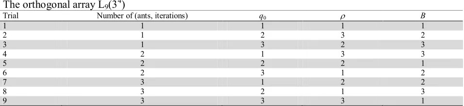
where the defuzzified value of the objective function is utilized as objective . It is noted that the terms ‘signal’ and ‘noise’ indicate the desirable value (response variable) and the undesirable value (standard deviation), respectively, and the purpose is to maximize the S/N ratio. Among the standard table of orthogonal arrays, L9(34) pattern presented in Table 2 is selected as the fittest design fulfilling the

necessary requirements.

Table 2

The orthogonal array L9(34)

Trial Number of (ants, iterations) q0  B

1 1 1 1 1

2 1 2 3 2

3 1 3 2 3

4 2 1 3 3

5 2 2 2 1

6 2 3 1 2

7 3 1 2 2

8 3 2 1 3

9 3 3 3 1

Finally, Table 3 summarizes the results, that is, the mean S/N ratios obtained at each level of the factors; the best levels of the factors are indicated in bold. Accordingly, the numeric parameters of the proposed ACO algorithm are set as follows: 20 ants in the colony, q0=0.99, =0.1 and B=10. In

Table 3

Results of the Taguchi method

Factor Level Mean S/N ratio

Number of (ants, iterations)

1 -52.076

2 -51.553

3 -51.925

q0

1 -51.788

2 -52.005

3 -51.772



1 -51.737

2 -51.818

3 -51.999

B

1 -52.219

2 -51.515

3 -51.820

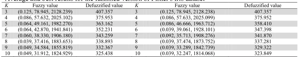
Furthermore, the computational results for the problem instances are shown in Table 4, which gives, for each number of clusters, the average and best objective function values achieved by the algorithm over ten independent runs, respectively.

Table 4

Average and best results for the fuzzified version of Fisher's Iris dataset

K Fuzzy value Defuzzified value K Fuzzy value Defuzzified value 3 (0.125, 78.945, 2128.239) 407.357 3 (0.125, 78.945, 2128.238) 407.357 4 (0.086, 57.632, 2025.102) 375.953 4 (0.086, 57.633, 2025.099) 375.952 5 (0.064, 49.161, 1982.270) 363.162 5 (0.086, 46.666, 1963.712) 358.410 6 (0.064, 42.870, 1941.841) 352.231 6 (0.039, 39.061, 1928.101) 347.398 7 (0.060, 38.330, 1906.180) 343.259 7 (0.092, 35.713, 1908.276) 341.870 8 (0.039, 37.416, 1883.653) 338.893 8 (0.039, 37.474, 1873.752) 337.281 9 (0.049, 34.584, 1855.819) 332.367 9 (0.039, 33.289, 1842.739) 329.322 10 (0.049, 31.912, 1824.929) 325.438 10 (0.039, 32.247, 1814.068) 323.849

From Table 4, as the best and average objective function values (particularly, the defuzzified values) are very close to each other for each number of clusters, it can be concluded that the proposed ACO algorithm is robust. Moreover, in view of the fact that the CPU time needed by the algorithm for each problem instance has never been more than 39 seconds, it seems that the algorithm is fast. Finally, it is noteworthy that the best results (over the ten runs) concerning the most plausible objective function value for the eight problem instances have been 78.945, 57.632, 46.666, 39.061, 35.713, 35.674, 33.289 and 28.917, respectively. Considering Eqs. (2-9), it is obvious that the most plausible value of the objective function depends only on the most plausible values of the object attributes (that is, the values in the original dataset). Then, comparing the above results with the optimal objective function values for the original non-fuzzy dataset, which for the eight numbers of clusters are 78.851, 57.228, 46.446, 39.040, 34.298, 29.989, 27.786 and 25.834, respectively (see Hansen et al., 2005), it can be concluded that the proposed algorithm is efficient. Of course, recall that the algorithm manages to minimize the defuzzified value of the objective function. In other words, if the algorithm managed to minimize the most plausible value of the objective function, it would be possible to attain even better results than those reported above.

5. Conclusions

rule based on the pheromone trails. If the constructed solution is infeasible, it is then replaced by a feasible solution by means of a straightforward repairing mechanism. To make the search more directed, the pheromone trails are dynamically modified according to a global updating rule. Moreover, the parameters of the algorithm are calibrated via the Taguchi method. Computational results show that the proposed algorithm is robust, fast and efficient.

References

Abbasbandy, S., & Hajjari, T. (2009). A new approach for ranking of trapezoidal fuzzy numbers.

Computers and Mathematics with Applications, 57, 413–419.

Ahmadizar, F., & Hosseini, L. (2012). Bi-criteria single machine scheduling with a time-dependent learning effect and release times. Applied Mathematical Modelling, 36, 6203–6214.

Ahmadizar, F., & Soltanpanah, H. (2011). Reliability optimization of a series system with multiple-choice and budget constraints using an efficient ant colony approach. Expert Systems with

Applications, 38, 3640–3646.

Al-Sultan, K.S. (1995). A tabu search approach to the clustering problem. Pattern Recognition, 28, 1443–1451.

Al-Sultan, K.S., & Fedjki, C.A. (1997). A tabu search-based algorithm for the fuzzy clustering problem. Pattern Recognition, 30, 2023–2030.

Bagirov, A.M. (2008). Modified global k-means algorithm for minimum sum-of-squares clustering problems. Pattern Recognition, 41, 3192–3199.

Bezdek, J.C. (1981). Pattern Recognition with Fuzzy Objective Function Algorithms. New York: Plenum Press.

Bloch, I. (1999). On fuzzy distances and their use in image processing under imprecision. Pattern

Recognition, 32, 1873–1895.

Brucker, P. (1978). On the complexity of clustering problems. in: Beckmenn, M., Kunzi, H.P. (Eds.), Optimization and Operations Research (Vol. 157). Berlin: Springer-Verlag, pp. 45–54.

Chang, D.X., Zhang, X.D., & Zheng, C.W. (2009). A genetic algorithm with gene rearrangement for K-means clustering. Pattern Recognition, 42, 1210–1222.

Chang, P.T., & Lee, E.S. (1994). Ranking of fuzzy sets based on the concept of existence. Computers

and Mathematics with Applications, 27, 1–21.

Chu, T., & Tsao, C. (2002). Ranking fuzzy numbers with an area between the centroid point and original point. Computers and Mathematics with Applications, 43, 111–117.

D’Urso, P., & Giordani, P. (2006). A weighted fuzzy c-means clustering model for fuzzy data.

Computational Statistics & Data Analysis, 50, 1496–1523.

Dorigo, M. (1992). Optimization, learning and natural algorithm. (in Italian). Ph.D. thesis, DEI, Politecnico di Milano, Itally.

Dorigo, M., & Gambardella, L.M. (1997). Ant colony system: A cooperative learning approach to the traveling salesman problem. IEEE Transactions on Evolutionary Computation, 1, 53–66.

Dorigo, M., & Stutzle, T. (2004). Ant Colony Optimization. London: Cambridge.

Fisher, R.A. (1936). The use of multiple measurements in taxonomic problems. Annals of Eugenics, 7, 179–188.

Gustafson, D.E., & Kessel, W.C. (1979). Fuzzy clustering with a fuzzy covariance matrix. in:

Proceedings of IEEE Conference on Decision and Control, San Diego, CA, pp. 761–766.

Handl, J., & Knowles, J. (2007). An evolutionary approach to multiobjective clustering. IEEE

Transactions on Evolutionary Computation, 11, 56–76.

Hansen, P., Ngai, E., Cheung, B.K., & Mladenovic, N. (2005). Analysis of global k-means, an incremental heuristic for minimum sum-of-squares clustering. Journal of Classification, 22, 287– 310.

Hung, W.L., & Yang, M.S. (2005). Fuzzy clustering on LR-type fuzzy numbers with an application in Taiwanese tea evaluation. Fuzzy Sets and Systems, 150, 561–577.

Hung, W.L., Yang, M.S., & Lee, E.S. (2010). A robust clustering procedure for fuzzy data. Computers

and Mathematics with Applications, 60, 151–165.

Jafari, H.R., Soltani, A.R., & Soltani, M.R. (2013). Measuring the performance of FCM versus PSO for fuzzy clustering problems. International Journal of Industrial Engineering Computations, 4, 387– 392.

Jain, A.K., Murty, M.N., & Flynn, P.J. (1999). Data clustering: A review. ACM Computing Surveys, 31, 264–323.

Kanade, P.M., & Hall, L.O. (2004). Fuzzy ant clustering by centroid positioning. in: Proceedings of

IEEE International Conference on Fuzzy Systems, Piscataway: IEEE Press, Vol. 1, pp. 371–376.

Kaufmann, A., & Gupta, M.M. (1991). Introduction to Fuzzy Arithmetic: Theory and Applications. London: International Thompson Computer Press.

Kim, D.S., & Kim, Y.K. (2004). Some properties of a new metric on the space of fuzzy numbers. Fuzzy

Sets and Systems, 145, 395–410.

Kivijarvi, J., Franti, P., & Nevalainen, O. (2003). Self-adaptive genetic algorithm for clustering.

Journal of Heuristics, 9, 113–129.

Likas, A., Vlassis, M., & Verbeek, J. (2003). The global k-means clustering algorithm. Pattern

Recognition, 36, 451–461.

Liu, Y., Yi, Z., Wu, H., Ye, M., & Chen, K. (2008). A tabu search approach for the minimum sum-of-squares clustering problem. Information Sciences, 178, 2680–2704.

MacQueen, J. (1967). Some methods for classification and analysis of multivariate observations. in:

Proceedings of 5th Berkeley Symposium on Mathematical Statistics and Probability, Berkeley:

University of California Press, Vol. 1, pp. 281–297.

Pappis, C.P., & Karacapilidis, N.I. (1993). A comparative assessment of measures of similarity of fuzzy values. Fuzzy Sets and Systems, 56, 171–174.

Phadke, M.S. (1989). Quality Engineering using Robust Design. Englewood Cliffs, NJ: Prentice-Hall. Pirzadeh, Y., Shahrabi, J., & Taghavifard, M.T. (2012). Rapid Ant based clustering-genetic algorithm

(RAC-GA) with local search for clustering problem. International Journal of Industrial Engineering

Computations, 3, 435–444.

Runkler, T.A. (2005). Ant colony optimization of clustering models. International Journal of

Intelligent Systems, 20, 1233–1251.

Shelokar, P.S., Jayaraman, V.K., & Kulkarni, B.D. (2004). An ant colony approach for clustering.

Analytica Chimica Acta, 509, 187–195.

Sun, L.X., Xie, Y.L., Song, X.H., Wang, J.H., & Yu, R.Q. (1994). Cluster analysis by simulated annealing. Computers & Chemistry, 18, 103–108.

Szmidt, E., & Kacprzyk, J. (2000). Distances between intuitionistic fuzzy sets. Fuzzy Sets and Systems, 114, 505–518.

Xiao, J., Yan, Y., Zhang, J., & Tang, Y. (2010). A quantum-inspired genetic algorithm for k-means clustering. Expert Systems with Applications, 37, 4966–4973.

Yang, M.S., Hwang, P.Y., & Chen, D.H. (2004). Fuzzy clustering algorithms for mixed feature variables. Fuzzy Sets and Systems, 141, 301–317.

Yang, M.S., & Ko, C.H. (1996). On a class of fuzzy c-numbers clustering procedures for fuzzy data.

Fuzzy Sets and Systems, 84, 49–60.

Yang, M.S., & Liu, H.H. (1999). Fuzzy clustering procedures for conical fuzzy vector data. Fuzzy

Sets and Systems, 106, 189–200.

Yang, M.S., & Wu, K.L. (2004). A similarity-based robust clustering method. IEEE Transactions on

Pattern Analysis and Machine Intelligence, 26, 434–448.