World Maritime University
The Maritime Commons: Digital Repository of the World
Maritime University
World Maritime University Dissertations
Dissertations
2000
Optimum container handling equipment plan in
Jakarta International Container Terminal (JICT) :
a quantitative model using interger linear
programming
Andi Isnovandiono
World Maritime University
Follow this and additional works at:
http://commons.wmu.se/all_dissertations
This Dissertation is brought to you courtesy of Maritime Commons. Open Access items may be downloaded for non-commercial, fair use academic purposes. No items may be hosted on another server or web site without express written permission from the World Maritime University. For more
Recommended Citation
Isnovandiono, Andi, "Optimum container handling equipment plan in Jakarta International Container Terminal ( JICT) : a quantitative model using interger linear programming" (2000).World Maritime University Dissertations. 57.
WORLD MARITIME UNIVERSITY
Malmö, Sweden
OPTIMUM
CONTAINER HANDLING EQUIPMENT PLAN
IN JAKARTA INTERNATIONAL CONTAINER
TERMINAL (JICT)
A Quantitative Model Using Integer Linear Programming
By
ANDI ISNOVANDIONO
The Republic of Indonesia
A dissertation submitted to the World Maritime University in partial
fulfillment of the requirements for the award of the degree of
MASTER OF SCIENCE
in
PORT MANAGEMENT
2000
DECLARATION
I certify that all the material in this dissertation that is not my own work has been
identified, and that no material included for which a degree has previously been
conferred on me.
The contents of this dissertation reflect my own personal views, and are not
necessarily endorsed by the University.
_____________________________ (Signature)
August 21st , 2000
Supervised by:
Professor Toshio Hikima
Associate Professor, Maritime Education and Training World Maritime University
Assessor:
Captain Jan Horck
Lecturer
World Maritime University
Co-assessor:
Gary Crook
Senior Economic Affairs Officer Transport Section
Division of Services Infrastructures for Development and Trade Efficiency
United Nations Conference on Trade and Development (UNCTAD)
DEDICATION
---
This work is sincerely dedicated to my employer, Indonesia Port
Corporation II, and all my family, who has supported me
---And
---
To my father Indaryadi, to my mother Soemartini, to my wife
---ACKNOWLEDGEMENTS
Words can not express my highest appreciation to all of those who have
contributed in one way or another to the success of my studies, particularly the
achievement of this dissertation. Therefore:
I would like to express my deep gratitude to His Excellency Mr. Herman
Prayitno, Managing Director of Indonesia Port Corporation II, and Mr. Harmani,
Human Resources and General Affairs Director of Indonesia Port Corporation II, for
nominating me as a participant to the Port Management Course at World Maritime
University (WMU) in Sweden.
Similarly, I would like to express my appreciation to Mr. Edi Waluyo, Training
and Education Body Secretary of Ministry of Communications for his excellent
co-ordination and kind co-operation.
I shall express my sincere and deep gratitude to the Tokyo Foundation for
awarding me a 21-month fellowship without which my studies at WMU would not
have been possible.
I shall be thankful to Dr. Ma Shuo, Professor of Port and Shipping
Management, for his special attention, advice, and directives, Dr. Bernard Francou,
and all other lecturers and professors at WMU as well as visiting professors for all
their advice, directives, and for sharing their immense knowledge and experience.
I wish to express my special thanks and appreciation to my supervisor
Professor Toshio Hikima, Associate Professor of Maritime Education and Training,
WMU and Inger Battista and other lecturers of English, for all their advice and
directives.
I would like to thank to Mr. Bruce Browne, Lyndell Lundahl, and personnel of
the Library, the Reception, Secretariat and all the Administration staff of WMU, for
I would like to thank to Hassan Ibrahim and Sajid Prijohutomo families for
their moral support before and during this period.
My deepest gratitude and appreciation to my lovely wife, Sita Ilona, for her
love and support during this period.
Finally, I am deeply grateful to my brothers, sisters, relatives and friends for
ABSTRACT
Title of Dissertation: Optimum Container Handling Equipment Plan in Jakarta
International Container Terminal (JICT) - A Quantitative
Model Using Integer Linear Programming
Degree: MSc
This dissertation discusses the procedures and ways to result the optimum
equipment plan in JICT. Its purpose is to evaluate the existing equipment and
propose the optimum container handling equipment plan to cope with the increase
of container traffic up to 2009 and to meet the equipment demands. Ultimately, it
will improve not only the performance and productivity but also the competitiveness
of the terminal. The following describes how the problem should be solved.
A careful forecasting procedure of container traffic is followed to minimise the
risks. It also considers the historical data of the container traffic and the changes in
the environment of the JICT such as economy, trade, and transport. The data
between 1994 and 1998 is used as a baseline for the forecast because of the data
availability. The result shows a valid and very good forecasting model having a
determinant (adjusted r2) of 0.98. The forecast result is then used to calculate the
equipment demands.
The equipment plan is done by using a mathematical method namely Integer
Linear Programming. By using this method, a mathematical model is built and an
optimum number of equipment needed is resulted with the minimum cost
configuration. So, the cost-benefit analysis has been incorporated into the model.
The model has also already considered a number of potential alternatives for having
a suitable equipment configuration to improve the quality of handling operations.
Next, the equipment plan model and the results is described and analysed.
Furthermore, the results are compared with traditional way of calculating it and
analysed as to plan the equipment acquisitions, investments, and policies and other
element related with the results, such as cost per move. The results derived from
the equipment plan model show a better equipment plan or configuration with lower
investments and total cost per move of container cranes.
Finally, some conclusions are made with emphasis on the procedures to
calculate an optimum equipment plan using an equipment plan model. A number of
recommendations to management and for further research are also made to be able
to implement the proposed equipment plan model.
Key words: JICT, Container handling equipment, Econometric approach, Container
traffic forecast, Trade and GDP, A mathematical model, Optimum
TABLE OF CONTENTS
Declaration ii
Dedication iii
Acknowledgements iv
Abstract vi
Table of Contents viii
List of Tables xii
List of Figures xiii
List of Abbreviations xv
1 Introduction
1.1 Overview 1
1.2 Identification of the problem 2
1.3 Objectives of the study 2
1.4 Scope of the study 3
1.5 Limitation of the study 3
1.6 Research methodology 3
1.7 Structure of the study 3
2 Selected country profiles and container terminal descriptions
2.1 Selected country profiles 5
2.1.1 Economy 5
2.1.1.1 Gross Domestic Product 6
2.1.1.2 Average currency rate 7
2.1.2 Trade 8
2.2 Container terminal descriptions 9
2.2.1 The hinterland and its connections 9
2.2.2 Container terminal throughput & ship calls 10
2.2.3 Container terminal handling system 11
2.2.5 Container terminal equipment 13
2.2.5.1 Number of equipment 13
2.2.5.2 Equipment performance 13
2.2.5.3 The age and conditions of equipment 15
2.2.5.4 Annual maintenance and running costs 16
2.3 The development of container handling equipment 17
2.4 Other selected profiles 17
2.5 Summary 17
3 Container traffic forecasting
3.1 Container traffic forecasting framework 18
3.2 Container traffic 19
3.3 Forecasting methodology 21
3.4 Determinants of container traffic 23
3.4.1 Export traffic 23
3.4.1.1 Transport sector 23
3.4.1.2 Trade sector 25
3.4.1.3 Economy sector 27
3.4.2 Import traffic 29
3.4.2.1 Transport sector 29
3.4.2.2 Trade sector 30
3.4.2.3 Economy sector 32
3.5 Container traffic forecasting model 34
3.6 Model validation 36
3.7 Scenarios 36
3.8 Container traffic forecasts 38
3.9 Analysis of the forecasts results 40
4 Container handling equipment planning
4.1 Mathematical modelling framework 41
4.2 The problem solving approach 42
4.2.1 Key concept 42
4.3 A mathematical model 44
4.3.1 Model formulation 44
4.3.1.1 Variables 44
4.3.1.2 Constraints 46
4.3.1.3 Objective function 47
4.3.2 Data needed to use the model 48
4.3.2.1 Handling rate 48
4.3.2.2 Daily demand for handling operations in quay side 49
4.3.2.3 Total annual costs 50
4.3.2.4 Capital costs of the equipment 51
4.4 The solution 52
4.5 The optimum equipment plan and acquisition policy 54
4.6 Summary 55
5 Analysis
5.1 Analysis of the optimum equipment plan model 57
5.2 Analysis of the optimum equipment plan 58
5.2.1 Container cranes 58
5.2.1.1 Existing equipment 58
5.2.1.2 New equipment 59
5.2.2 Other container handling equipment 60
5.3 Investments 60
5.4 Cost per move of container cranes 62
5.5 Comparison between traditional way and the model 62
5.6 Summary 64
6 Conclusions and recommendations
6.1 Conclusions 65
6.2 Recommendations 67
6.2.1 Recommendations to JICT 67
6.2.2 Recommendations for further research 67
Appendices
Appendix 1 The age and conditions of the equipment (September 1999) 72
Appendix 2 Correlation between container traffic and other related data
(base year: 1994 – 1998) 77
Appendix 3 Number of container movements of forecasted container traffic
(2000 - 2009) 78
Appendix 4 Economic life calculation of equipment (container cranes) 79
Appendix 5 Summary of optimal solutions using Quant System 3.0 software 92
Appendix 6 Optimal container handling equipment plan (2000 - 2009) 108
Appendix 7 The comparison of number of container cranes needed,
cost per move, and capital investment needed between
LIST OF TABLES
Table 2.1 Indonesia merchandise trade (1994 – 1998) 9
Table 2.2 Container traffic in Jakarta International Container Terminal
in TEU and Ton (1994 – 1999) 11
Table 2.3 Container terminal facilities 12
Table 2.4 Age of equipment (units) 15
Table 2.5 Annual maintenance and running costs of equipment 16
Table 3.1 Regression summary result for the aggregate model 34
Table 3.2 Economic scenarios based on the historical data 38
Table 3.3 Container traffic forecasts for year 2000 – 2009 38
Table 4.1 Decisions on equipment 43
Table 4.2 Handling rate of equipment (container cranes) 49
Table 4.3 Daily demand of container moves 49
Table 4.4 Annual total costs 51
Table 4.5 Number of new container cranes needed and its investments 53
LIST OF FIGURES
Figure 2.1 Indonesia GDP and its annual percentage changes (1994 – 1998) 6
Figure 2.2 Agriculture/manufacturing share of Indonesia GDP (1980/1997) 7
Figure 2.3 Indonesia currency value and its depreciation (1994 – 1998) 8
Figure 2.4 Indonesia merchandise trade in value and its shares (1994 – 1998) 8
Figure 2.5 Map of hinterland of the container terminal 10
Figure 2.6 The number of equipment in JICT 1999 13
Figure 2.7 Equipment performance in JICT 1999 14
Figure 3.1 Container traffic forecasting framework 19
Figure 3.2 Container traffic import and export (in TEU) 20
Figure 3.3 Containerized traffic import and export (in Ton) 20
Figure 3.4 Level of influence to the port 22
Figure 3.5 Relationships between export of containerized traffic, fleet
capacity and ship calls (1994 – 1998) 24
Figure 3.6 Export values and shares of seven main destination countries
(January – October 1999) 25
Figure 3.7 Relationships between export of containerized traffic and export
trade in values (1994 – 1998) 26
Figure 3.8 Relationships between export of containerized traffic and East Asia
trade volume growth and trade volume change per annum
(1994 – 1998) 27
Figure 3.9 Relationships between export of containerized traffic and real
GDP growth of the country and GDP development in Asia
(1994 – 1998) 28
Figure 3.10 Relationships between export of containerized traffic and the
value of local currency rate per USD (1994 – 1998) 29
Figure 3.11 Relationships between import of containerized traffic, fleet
capacity and ship calls (1994 – 1998) 30
Figure 3.12 Relationships between import of containerized traffic and import
Figure 3.13 Import values and shares of seven main countries of origins
(January – October 1999) 31
Figure 3.14 Relationships between import of containerized traffic and East Asia
trade volume growth and trade volume change per annum
(1994 – 1998) 32
Figure 3.15 Relationships between import of containerized traffic and GDP
of the country (1994 – 1998) 33
Figure 3.16 Relationships between import of containerized traffic and real
GDP growth of the country and GDP development in Asia
(1994 – 1998) 33
Figure 3.17 Relationships between import of containerized traffic and the
value of local currency rate per USD (1994 – 1998) 34
Figure 3.18 Comparison of containerized traffic, in Ton and TEU
actual v.s. model (1994 – 1999) 36
Figure 3.19 Container traffic actual (1994 – 1999) and forecasted
(2000 – 2009) in TEU 39
Figure 4.1 Mathematical modeling framework 41
Figure 4.2 The comparisons of the number of container cranes needed with
different utilisation scenarios 54
Figure 5.1 The comparisons of the results between traditional way and
LIST OF ABREVIATIONS
ADB Asian Development Bank
CC Container Crane
CFS Container Freight Station
CY Container Yard
EDI Electronics Data Interchange
FD Forklift Diesel
GDP Gross Domestic Product
HMC Harbor-Mobile Crane
HPH Hutchinson Port Holdings
HT Head Truck
ICBS Indonesian Central Bureau of Statistics
IMF International Monetary Fund
ITC International Trade Center
JICT Jakarta International Container Terminal
KOPEGMAR Koperasi Pegawai Maritim (Maritime Employee’s Co-operative)
RTG Rubber-Tyred Gantry Crane
TEU Twenty Feet Equivalent Units
UNCTAD United Nations Conference of Trade and Development
USA United States of America
USD United States of America Dollar
USDOC United States Department of Commerce
CHAPTER 1
Introduction
“This chapter describes the overview, identification of the problems, objectives, scope, limitations, research methodology and structure of this study”
1.1 Overview
On April 1999, Hutchinson Port Holdings (HPH) completed the purchase of a 51%
stake in the newly formed Jakarta International Container Terminal (JICT) from
Indonesia Port Corporation II (IPC II) and IPC II’s employee cooperative, Koperasi
Pegawai Maritim (Kopegmar).
JICT has been formed to operate container terminals I and II at Tanjung
Priok Seaport for a period of 20 years, to upgrade its facilities and systems to world
class standards, and to undertake the construction and development of additional
container handling capacity adjacent to container terminal I. The upgrading and
expansion of JICT will further contribute to the country’s economic development in
facing the globalisation of the world economy and trade liberalisation.
Globalisation of the world economy and trade liberalisation has increased the
global general cargo and container volumes. As stated in his article, Peters (BIMCO
Review 2000, p.26) “the global general cargo and container volumes will continue to
grow for many years to come”. This also happened to JICT (formerly container
terminals I and II), which is the largest container terminal in Indonesia and is one of
the country’s most important economic gateways, where the container traffic grew
dramatically from 0.18 million TEUs in 1986 to 1.53 million TEUs in 1997 or more
than eight times. Although this growth slightly decreased in 1999 to 1.47 million
TEUs due to the post economic crisis in Indonesia, it is believed that the container
Introduction
---Despite that situation, JICT also has to fulfil the vision and mission of its
mother company, IPC II, which is to be a world-class port operator. To achieve it,
JICT should continuously provide high quality services as close as possible to the
customer requirements. In order to do so, it is important to have an adequate
inventory of the equipment, so the terminal can meet cargo handling needs and
achieve its operational performance targets. In addition, “investment in port
infrastructure and equipment is expensive and, given the highly dynamic and
competitive nature of the maritime business, inherently risky” (McDonagh, 2000,
p.24). Therefore, JICT needs to have a medium or long-term equipment plan to
ensure that high quality services are being achieved with the minimum risks.
1.2 Identification of the problems
Preparing an equipment plan for the port is a complex process and full attention
must be allocated to it. Furthermore, the accuracy of the equipment plan itself
depends on the accuracy of the data available. If the data is not accurate, it can
mislead the results. In addition, the planning process has to be carefully managed
and prepared to minimise the risks. These risks can be limiting the future growth of
container traffic and over-investment in equipment.
This study is trying to answer the following questions: How to deal with these
risks? What problems do exist in relation with these risks? How to minimise these
risks? How to determine the adequate (optimum) inventory of the equipment? What
is the impact on the future of the container trade regarding investments, or costs per
move? What actions should be taken to succeed the implementation of this study?
1.3 Objectives of the study
Based on the background described in the previous paragraph, this study has the
following general objectives:
To ensure that the port has an adequate number of container handling
equipment to cope with the increase in container traffic;
Introduction
To give guidelines to management in applying equipment acquisition policies
and investments;
To provide management with a tool to calculate the optimum container handling
equipment plan.
1.4 Scope of the study
The scope of the study is limited to determining the container handling equipment
plan in JICT.
1.5 Limitation of the study
This study does not discuss the maintenance policies and procedures
comprehensively but discusses how to determine the optimum container handling
equipment plan. The optimum number of equipment is based on the assumption that
the availability is set at a certain level. It means that there will be higher cost for
preventive maintenance to achieve such availability of the equipment.
1.6 Research methodology
For this study, the primary data was collected directly from the company and the
secondary data was collected from various sources (reports, magazines, internet).
Literature research was done in the library to gain necessary information. In
addition, the equipment planning process was done according to UNCTAD (1990,
pp. 40-41). Furthermore, to have an optimum container handling equipment, the
problem was solved by a mathematical model using integer linear programming
approach using a Quant System software.
1.7 Structure of the study
Normally when dealing with planning, there are three main modules that should be
dealt with, namely forecasting, planning, and simulation. In this dissertation, the
author clearly does two of them: container traffic forecasting (Chapter 3) and
equipment planning (Chapter 4). The latter, simulation, is done by applying
scenarios in the forecasting and equipment planning process. Therefore, for the
Introduction
---Chapter 1 Introduction. This chapter describes the overview, identification of
the problems, objectives, scope, limitation, research methodology, and the structure
of the study.
Chapter 2 Selected country profiles and container terminal descriptions. This
chapter describes the information of particular country profiles and the container
terminals in JICT including the throughput, handling system, equipment types,
numbers, performances, the age, conditions, annual maintenance and running
costs, and the recent development of container handling equipment to see the
possibilities to apply this new development of container handling equipment. The
country profiles and the terminal throughput is used to forecast the container traffic
and, ultimately, to calculate the optimum equipment plan.
Chapter 3 Container traffic forecasting. This chapter describes and
discusses the container traffic forecast methodology and the factors affecting the
container traffic to be able to have reliable container traffic forecast by using a
specific statistical method (an econometric approach).
Chapter 4 Container handling equipment planning. This chapter describes,
discusses, and analyses the framework of the equipment planning process, the
operational scenarios, and how this problem can be solved by a mathematical
approach using integer linear programming.
Chapter 5 Analysis. This chapter discusses and analyses the optimum
equipment plan model, its results, and its implications to costs per move of container
cranes, the company’s investments and the comparisons between the traditional
way and the equipment plan model of calculating the equipment plan.
Chapter 6 Conclusions and recommendations. This chapter describes the
conclusions of the study and gives the recommendations to the management of
CHAPTER 2
Selected country profiles and
container terminal descriptions
“This chapter describes selected country profiles, container terminal descriptions, and the development of container handling equipment and discusses them”
2.1 Selected country profiles
Basically, the selected country profiles discussed are economy and trade sectors.
These profiles are needed to forecast the container traffic in the future.
2.1.1 Economy
Prior to independence, Indonesia's economy was oriented to providing raw materials
to the Netherlands. Subsistence agriculture, primarily the production of rice, was the
mainstay of most of the population; but the economy also relied on plantation
agriculture, including the production of sugar and rubber. Industry was not promoted
so as to avoid competing with the Netherlands.
In the 1970s, the economic policy was to expand foreign investment and
increase trade. When export revenues from oil declined in the early and mid-1980s,
Indonesia was forced to expand other exports. To make these exports more
competitive internationally, the government deregulated parts of the economy such
as coastal transportation, finance, and banking.
Indonesia's economy grew impressively during the 1980s and much more in
the 1990s, largely on the strength of its natural resources, which include a large
Selected Countr y Profiles and Container Terminal Descriptions
---2.1.1.1 Gross Domestic Product
Indonesia's gross domestic product (GDP) was USD 227 billion in 1996, the largest
in Southeast Asia. Between 1994 and 1996, the GDP grew by about 30.9%.
Between 1994 and 1996, the growth was always positive with an average growth
13.3%. But in mid-1997 an economic crisis developed in Asia whereby investors
lost confidence in certain debt-laden economies. As the crisis spread to Indonesia,
the value of the Indonesian currency plummeted, which threatened the capacity of
the government, banks, and businesses to repay their foreign debts. As an impact,
the GDP growth fell to negative (-5.1%) and even much worse in 1998 when the
growth sharply declined to –56.4% (see Figure 2.1).
In addition, between 1980 and 1997 there were significant shifts in the structure of
the Indonesian economy. Agriculture shrunk from 41 to 24 percent. The industry as
a whole remained stable, but manufacturing, the largest component of the industry,
grew from 13 to 25 percent of the GDP (see Figure 2.2). Consequently, Indonesia
is more dependent on manufacturing as its main economy sources. Therefore, as a
result of this crisis, in the period of January and October 1999, ”the manufacturing
product export values increased by USD 2.67 billions (or 13.80%) to USD 21.99
billions but import values decreased by USD 4.41 billions (or 27.28%)” (ICBS, 1999) compared with the same period the year before.
173.74 196.01 227.4
215.78
94.15 -5.11%
-56.37% 16.02%
12.82% 11.16%
0 50 100 150 200 250
1994 1995 1996 1997 1998
U
S
D
Billion
-60% -50% -40% -30% -20% -10% 0% 10% 20%
Perc
entage
(Year-ov
e
r-Year)
GDP Annual % change
Figure 2.1
Indonesia GDP and its annual percentage change
(1994 – 1998)
Selected Countr y Profiles and Container Terminal Descriptions
---2.1.1.2 Average currency rate
Indonesia's currency value (Rupiah) sharply weakened in 1998 with the depreciation
of about 71% from the 1997 value following the economic crisis which commenced
in mid-1997 (see Figure 2.3). However, in 1997, Rupiah, based on average
currency rate experienced depreciation of only about 19% from the previous year.
In addition, between 1994 and 1998, the depreciation was about 78%. Many
analysts discussed that the economic crisis spread was caused by several factors of
influence, as Michel Camdesus reported in its Asia-Europe Finance Ministers
Meeting in Frankfurt, Germany, January 16, 1999:
Four influences may explain this phenomenon:
(i) common factors in the external environment, specifically the
features in the global financial system that led to the large flows of
volatile capital to the region;
(ii) the spillover effects from trade and financial linkages among the
countries;
(iii) a true contagion effect, as the crisis in one country caused
investors to reassess the fundamentals in other countries; and
(iv) a number of unexpected exogenous factors, including weaker
terms of trade and the deepening of the recession in Japan.
41% 13% 24% 25%
78
215
0 50 100 150 200 250
1980 1997
U
S
D
Billion
0% 10% 20% 30% 40% 50%
Agric
u
lture/M
anufac
turing
as
Perc
ent of G
D
P
Agriculture Manufacturing GDP
Figure 2.2
Agriculture/manufacturing share of Indonesia GDP
(1980/1997)
Selected Countr y Profiles and Container Terminal Descriptions
---2.1.2 Trade
Indonesia’s trade share between imports and exports between 1994 and 1997 was
relatively stable (44% and 56% respectively). But in 1998, the import share was
lower (36%) compared with the average share between 1994 and 1997 as the Asian
crisis deepened. Exchange rate variations (the value of the Indonesian currency
plummeted), which were large in the course of 1998, can have a major impact on
the dollar prices of internationally traded goods. The impact is that import goods
becomed more expensive and export goods becomed cheaper. That is why the
total Indonesia’s trade in value fell in 1998, particularly sharply for import trade (see
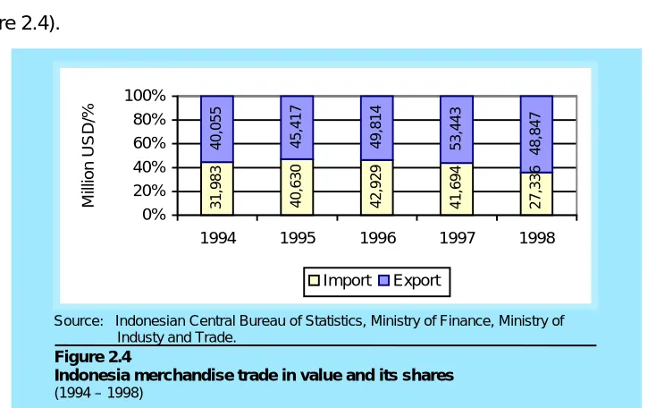
Figure 2.4). 40, 055 45, 417 49, 814 31, 983 40, 630 42, 929 41, 694 27, 336 53, 443 48, 847 0% 20% 40% 60% 80% 100%
1994 1995 1996 1997 1998
M illio n USD/% Import Export Figure 2.4
Indonesia merchandise trade in value and its shares
(1994 – 1998)
0 2,000 4,000 6,000 8,000 10,000 12,000
1994 1995 1996 1997 1998
Rupiah per US
D -80% -60% -40% -20% 0% Depreciation (Y ear-over-Y ear)
Currency value Depreciation
Figure 2.3
Indonesia currency value and its depreciation
(1994 – 1998)
Source: Indonesian Central Bureau of Statistics, Bank Indonesia, Ministry of Finance, World Bank, U.S. Department of Commerce (USDOC).
Selected Countr y Profiles and Container Terminal Descriptions
---Tabel 2.1
Indonesia merchandise trade
(1994 – 1998)
Source: Indonesian Central Bureau of Statistics, Ministry of Finance, Ministry of Industy and Trade.
In terms of value, the import trade growth in 1998 declined to -34% whilst the export
trade declined to -9% (see Table 2.1). This import and export trade growth
decreased sharply as compared with the average trade growth in 1994-97 (11% and
10% respectively). However, the import value in 1998 was still slightly above the
import value in 1992 (i.e. USD 27,279 million).
Million USD
% Annual Change
Descriptions 1994 1995 1996 1997 1998
1994 1995 1996 1997 1998
1994/97
Average
Total Trade 72,038 86,047 92,743 95,137 76,183 11% 19% 8% 3% -20% 10%
Import Trade 31,983 40,630 42,929 41,694 27,336 13% 27% 6% -3% -34% 11%
Export Trade 40,055 45,417 49,814 53,443 48,847 9% 13% 10% 7% -9% 10%
2.2 Container terminal descriptions
2.2.1 The hinterland and its connections
The terminal is serving the most rapid growing hinterland area of the country from
the utmost western side of Java Island until the border of Central Java. Its posistion
is very strategic, surrounded by many industrial areas and some plantations. The
western part is mainly industrial areas situated in Merak, Cilegon and Tangerang.
The central and eastern parts are also industrial areas situated in Jakarta and
Bekasi. In the southern part beginning from Cibinong, Bogor, Sukabumi, Cianjur
and Bandung, there are some plantation areas that produce tea, rubber, rice, fruit
and other commodities (Port of Tanjung Priok, 1997).
The terminal is connected to its hinterland by roads and railway systems as
shown in Figure 2.5. The railway connections are dedicated to transport a number
of particular commodities between the terminal to the inland port of Gede Bage in
Bandung, the capital of West Java. The railway service is provided by a railway
Selected Countr y Profiles and Container Terminal Descriptions
---Figure 2.5 Map of hinterland of the container terminal (Port of Tanjung Priok)
2.2.2 Container terminal throughput & ship calls
Container throughput in JICT is always increasing, as the world container market
grows continously, except in 1998 and 1999 due to the economic crisis in Indonesia.
Between 1994 and 1997, the traffic increased by almost 32% from 1.16 million TEUs
to 1.53 million TEUs, while in terms of tons, the traffic increased by 27% from 10.43
to 13.29 million tons. However, because of the economic crisis, the traffic slightly
decreased to 1.42 and 1.47 million TEUs or, in terms of tons, decreased to 10.59
and 12.63 million tons in 1998 and 1999 respectively (see Table 2.2).
In 1994, the number of ship calls was about 2,000 calls with an average load
of 600 TEUs per ship. Furthermore, between 1995 to 1998, the number of ship calls
was decreasing to around 1,600 calls, but the average load was increasing to 900
TEUs per ship. It means that, after 1994, the ship size was increasing as the
Selected Countr y Profiles and Container Terminal Descriptions
---Table 2.2
Container traffic in Jakarta International Container Terminal in TEU and Ton
(1994 – 1999)
Descriptions 1994 1995 1996 1997 1998 1999
Shipcalls 1,984 1,492 1,574 1,665 1,580 1,588
% change -1.05% -24.80% 5.50% 5.78% -5.11% 0.51%
TEU Import 564,706 642,788 700,943 755,373 698,474 730,463
TEU Export 599,426 657,338 723,140 777,704 726,473 742,042
In TEU (Total) 1,164,132 1,300,126 1,424,083 1,533,077 1,424,947 1,472,505
% change 18.99% 11.68% 9.53% 7.65% -7.05% 3.34%
Ton Import 5,851,839 6,855,499 7,236,660 7,481,625 4,112,794 6,093,383
Ton Export 4,576,894 5,329,317 6,201,285 5,807,825 6,472,808 6,536,776
In Ton (Total) 10,428,733 12,184,816 13,437,945 13,289,450 10,585,602 12,630,159
% change 16.39% 16.84% 10.28% -1.11% -20.35% 19.31%
2.2.3 Container terminal handling system
According to its operational features, JICT is using the rubber-tyred gantry
crane (RTG) system for its operation. In this system, “the container yard is equipped
with rubber-tyred gantry cranes for stacking and unstacking, with tractor-trailer units
for quay transfer and other movements” (UNCTAD, 1986a, p. 5). Transfer between
shipside and CY is carried out by tractor-trailer sets.
The RTGs pick up the containers from the roadway and move along the row
to stack them in the CY while the trucks-trailer sets move off around the CY and
back to the quay apron. For receipt/delivery, road vehicles are allowed onto the
terminal and along the truck lane to the appropriate row. The RTGs are used solely
for stacking/unstacking and moving positions within the row in the block. The
terminal is also using Harbour-Mobile Cranes (MHC) to load and unload containers
to and from the trucks or trailers on the quay apron, but they are not very much in
use.
Selected Countr y Profiles and Container Terminal Descriptions
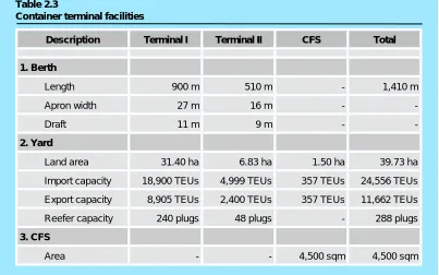
---Table 2.3
Container terminal facilities
In the CFS, the equipment used is forklifts with various capacities. After
stripped and stuffed in the CFS, forklifts move containers to the tractor-trailers. The
tractor-trailers then move them to the CY or out of the terminal. For a particular
case, container handling is done by top loader or side loader. This operation is
normally done to receive export empty containers from the external trailers.
The terminal is operated 24 hours a day and seven days a week with three
shifts. The terminal implemented EDI to improve its services on 15 September 1997.
In other cases, for the clients who have not implemented EDI, the terminal also
provides a Help Desk to assist them.
2.2.4 Container terminal facilities
In total, the JICT has a total quay length of 1,410 m comprising six berths with
alongside depth from –9m to –11m, whilst the seventh berth currently being
equipped has a depth of –14 m. The total container yard area is 39.73 ha with an
import capacity of 24,556 TEUs and an export capacity of 11,662 TEUs. Although
export traffic is higher than import traffic, the import capacity is higher due to the
longer dwelling time. The total CFS area is 4,500 sqm. Those figures are shown in
Table 2.3.
Description Terminal I Terminal II CFS Total
1. Berth
Length 900 m 510 m - 1,410 m
Apron width 27 m 16 m -
-Draft 11 m 9 m -
-2. Yard
Land area 31.40 ha 6.83 ha 1.50 ha 39.73 ha
Import capacity 18,900 TEUs 4,999 TEUs 357 TEUs 24,556 TEUs Export capacity 8,905 TEUs 2,400 TEUs 357 TEUs 11,662 TEUs
Reefer capacity 240 plugs 48 plugs - 288 plugs
3. CFS
Selected Countr y Profiles and Container Terminal Descriptions
---2.2.5 Container terminal equipment
2.2.5.1 Number of equipment
Terminal I is served by 8 container cranes (CCs), 3 mobile harbour cranes (MHCs),
30 rubber-tyred gantry cranes (RTGs), 10 forklift diesel (FDs), 56 head-truck (HTs)
and 63 chassis. Terminal II is served by 4 CCs, 1 MHC, 14 RTGs, 3 FDs, 15 HTs
and 29 chassis (Unit Terminal Petikemas Tanjung Priok, p. 28). So in total, the JICT
is served by 12 CCs and 4 MHCs, 44 RTGs, 17 FDs, 71 HTs and 92 chassis (see
Figure 2.6).
Among the cranes there are some leased equipment. For the CC, there are
3 pieces of leased equipment in terminal II. For the MHC, all of the equipment is
leased equipment. For the RTG, there are 9 pieces of leased equipment in terminal I
and 3 pieces of leased equipment in terminal II.
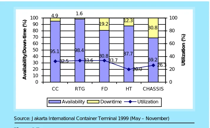
2.2.5.2 Equipment performance
The JICT measures the performance of equipment by taking into account the
achievement of availability, downtime, and utilisation of equipment. UNCTAD also
considers these indicators as very important measures for equipment performance.
Figure 2.6
The number of equipment in JICT 1999
Source: Jakarta International Container Terminal 1999.
8 3
30
10
56 63
4 1
14
5
15
29
12
4
44
15
71
92
0 20 40 60 80 100
CC MHC RTG FD HT
CH ASSIS
Un
its
Selected Countr y Profiles and Container Terminal Descriptions
---Although the JICT divides availability of equipment into three different parts,
i.e., availability equipment, availability inherent and availability occupied, for the
purpose of this study, the performance of equipment is measured according to
formulas introduced by UNCTAD (1990, p.3), such as: equipment availability,
equipment down-time, and equipment utilisation.
Equipment availability is defined as a measure of proportion of time
individual machines or classes of machines, which are accessible to operators.
Equipment downtime is defined as a measure of the time when equipment is out of
service and unavailable for use. Equipment utilisation is defined as a measure of proportion of the time that a machine (or category of machines) is performing useful
work. The performance of the equipment by category in the JICT is described in
Figure 2.7.
In general, all the equipment has a very good availability that is about 80 to
98%, except for chassis, which has the availability of 70%. In terms of utilisation,
the utilisation of the RTG, head truck and chassis is lower compared with the
average utilisation recommended by UNCTAD. However, this does not show the
real situation since this data is based on a five-month observation. Since all MHCs
are leased equipment, its performance is not shown in Figure 2.7.
95.1 98.4 80.8 87.7 69.2 4.9 1.6 19.2 12.3 30.8
32.5 33.6 33.7
20.0 26.3 0 10 20 30 40 50 60 70 80 90 100
CC RTG FD HT CHASSIS
A v a ila bilit y /D o w n -t im e ( % ) 0 20 40 60 80 100 U tiliz a tion ( % )
Availability Downtime Utilization
Figure 2.7
Equipment performance in JICT 1999
Selected Countr y Profiles and Container Terminal Descriptions
---Table 2.4
Age of the equipment (units)
2.2.5.3 The age and conditions of equipment
Equipment owned by JICT varies in brand/manufacturer and age due to the different
sources of funding. This condition is normal in developing countries because there
is lack of money for funding their equipment, which usually needs a huge
investment. In the following, the author is trying to explain the age and conditions
for each type of equipment in general.
There are three container cranes over 20 years old, one between 11 to 20
years old, and five containers below 10 years old. It can be said that 44% of the CCs
are quite old equipment and constitute the main hindrance to its efficiency. In
addition, there are seven RTGs over twenty years old, eight RTGs between 11 to 20
years old, and seventeen RTGs below 10 years old. The situation is better where
more than 50% of the RTGs are still ‘young’.
Furthermore, for forklift diesel, one of them is over 20 years old, seven of
them between 11 to 20 years old and nine of them are below 10 years old.
Moreover, for the head-truck, thirteen of them are between 11 to 20 years old,
forty-eight of them are between 5 to 10 years old and ten of them are below 5 years old.
This equipment is quite new, reliable and operational.
Finally, for chassis, fourteen of them are over 20 years old, eighteen of them
are between 11 to 20 years old, fifty of them are between 5 to 10 years old, and ten
of them are below 5 years old. The age breakdown for each type of the equipment
is as follows.
Type of Equipment < 5 years 5 to 10
years
11 to 20 years
> 20 years Total
Container Crane 2 3 1 3 9
Transtainer (RTG) - 17 8 7 33
Fork-lift Diesel 6 3 7 1 17
Head Truck 10 48 13 - 71
Chassis 10 50 18 14 92
Selected Countr y Profiles and Container Terminal Descriptions
---Table 2.5
Annual maintenance and running costs of equipment
Source: Company record.
Exchange rate: 1USD = Rp. 8,000,- (1998) and Rp. 8,000,- (1999)
2.2.5.4 Annual operating (maintenance and running) costs of equipment
For the purpose of the equipment plan model, annual operating costs of equipment
are taken only for container cranes. The percentage changes in USD are the same
with the changes in Rupiah, that is between 10 to 17% annualy because the
exchange rate applied by the company is the same i.e. Rp 8,000 per USD.
However, these changes do not really represent the actual increase in annual
operating costs because , in facts, the exchange rate is different. The increase in
costs is calculated based on the assumption that maintenance cost changes
increase as the age of equipment become older. The 1999 operating cost data, as
shown in Table 2.5 were used as a base for further calculation. The complete
calculation of the economic life or annual costs of the equipment (capital recovery
and operating costs) is shown in Appendix 3.
From Table 2.5, it can be concluded that, coincidently, the changes of the
operating costs per year of equipment are typical for particular groups of equipment.
For example: 1970’s Pre-Panamax cranes have annualy operating costs changes of
around 10 to 11%. In addition, 1990’s Panamax cranes have annual maintenance
and running costs changes of around 17%.
Year Maintenance Costs
(in Indonesian Rupiahs)
Maintenance Costs (in USD) Equipment
Register
made Used 1998 1999
%
change
1998 1999
% change
CC02A (2nd) 1972 1992 209,317,380 233,078,335 11.35% 26,165 29,135 11.35% CC02 1976 1978 470,814,358 519,972,914 10.44% 58,852 64,997 10.44% CC03 1976 1978 499,425,532 549,691,727 10.06% 62,428 68,711 10.06% CC01 1983 1986 314,355,391 386,923,807 23.08% 39,294 48,365 23.08% CC04 1992 1992 979,252,905 1,145,075,800 16.93% 122,407 143,134 16.93% CC05 1992 1992 1,096,625,284 1,282,467,582 16.95% 137,078 160,308 16.95% CC06 1992 1992 1,052,767,288 1,231,087,227 16.94% 131,596 153,886 16.94% CC07 1997 1997 963,839,304 1,128,202,686 17.05% 120,480 141,025 17.05% CC08 1997 1997 914,094,454 1,074,667,511 17.57% 114,262 134,333 17.57%
Selected Countr y Profiles and Container Terminal Descriptions
---Table 2.5 also shows that the Panamax cranes have higher annual operating
costs than the Pre-Panamax cranes, although Panamax cranes are much ’younger’
than Pre-Panamax cranes. It can be explained because each piece of equipment
has its own specifications e.g. horse power, etc., which affect the increases of the
costs. For example: for a particular manufacturer, the machine or drive of the
equipment is not ’suitable’ in tropical climates, where the machines are often having
problems with the engine so spares from the manufacturer country for repairs, are
needed, which is expensive. On the other hand, for another particular manufacturer,
the drive of the equipment is more reliable and needs less money to maintain.
Uitlization of the individual equipment also affects the increase in costs.
2.3 The development of container handling equipment
In general, “the trend will be for container handling equipment to be cheaper to
maintain which will increase its economic life but probably no more than 20 per cent”
(Crook, 2000). It also means that the price of equipment may be cheaper with
higher handling rate per hour. In specific cases, the container crane sizes will be
bigger and bigger “dictated by increases in vessel size (notably of beam and
freeboard) and container dimensions“ (UNCTAD, 1986a, p. 24).
2.4 Other selected profiles
The other selected profiles are considered as other factors influencing the container
traffic other than the previous ones. Those factors are container shipping fleet
capacity, East Asia trade volume growth, Asia’s trade volume change per annum,
and GDP development in Asia. The profiles are shown in Appendix 2.
2.5 Summary
This chapter has clearly described the selected country profiles and container
terminal descriptions, which are important for this study. The data of selected
country profiles, container terminal figures, and other selected profiles are used to
forecast the containerised traffic using econometric approach. In addition, some container terminal descriptions are used in relation to the equipment planning for the
CHAPTER 3
Container traffic forecasting
“This chapter describes the container traffic forecasting and discusses the methodology used for its forecast”
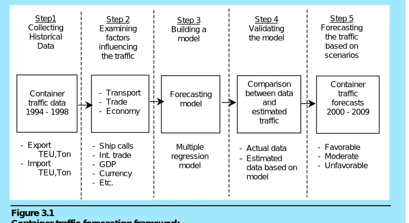
3.1 Container traffic forecasting framework
To determine the optimum container handling equipment plan for long-term (i.e. ten
years) planning, there has to be the procedure to deal with it. The container
handling equipment needs depend on the container traffic. Therefore, a forecasting
system to forecast the container traffic is needed in order to determine how much
equipment is necessary. The implementation of a forecasting system requires:
(1) identification of key environmental sectors (by correlation analysis);
(2) forecasting of key environmental sectors (by looking at a reliable sources);
(3) conditional forecasting for alternative strategic option (by scenarios)
(Makridakis, Wheelwright, 1987, p.80).
To apply the procedure, it is important to identify the key environmental
factors influencing container traffic. There are several causal relationships and
factors that affect container traffic. The author identified that transport, trade, and
economy is the environmental factors influencing the port (i.e. container traffic). To
determine the relationships between container traffic and these environmental
factors, an examination of the variables quantifying those environmental factors is
required. For the various relationships between the container traffic and its
variables, some variables will typically have a more important impact than others.
The correlation between the container traffic and its variables will show this. The
Container Traffic Forecasting
---Figure 3.1
Container traffic forecasting framework
Container traffic data 1994 - 1998
Forecasting model Comparison between data and estimated traffic Step 2 Examining factors influencing the traffic Step1 Collecting Historical Data Step 3 Building a model Step 5 Forecasting the traffic based on scenarios Step 4 Validating the model Container traffic forecasts 2000 - 2009 - Transport - Trade - Economy - Export TEU,Ton - Import TEU,Ton
- Ship calls - Int. trade - GDP - Currency - Etc. Multiple regression model
- Actual data
- Estimated data based on model
- Favorable - Moderate - Unfavorable
After examining those variables, a forecasting model of container traffic can be build
by using multiple regression analysis (simultaneous system). This model has a
major advantage, that is it can explain inter-relationships between dependent
variables. This approach is used because the author wants to have explanatory
variables influencing the container traffic. The framework for container traffic
forecasting is described on Figure 3.1.
3.2 Container traffic
Container traffic in terms of TEU and Ton (see Figures 3.2 and 3.3) in JICT have
continuously increased from year to year (except in 1998 as an impact of the
economic crisis and it still affected growth in 1999). However, the trends in general
are constantly increasing as a result of containerisation.
This continued increase in container traffic is widely expected and the port
needs to anticipate this increase by planning port expansion i.e. container handling
Container Traffic Forecasting
---Figure 3.2
Container traffic import and export
(in TEU)
Figure 3.3
Containerised traffic import and export
(in TON)
Data for container traffic is taken in terms of TEU and Ton (containerised). It is also
divided into imports and exports to see the proportion of this container traffic based
on its activity. The figures are based on the container traffic data between 1994 and
1999 (see Table 2.2).
564,706 642,788 700,943 755,373 698,474 730,463 599,426 657,338 723,140
777,704 726,473 742,042 1,164,132 1,300,126
1,424,083 1,533,077 1,424,947 1,472,505
0 500,000 1,000,000 1,500,000 2,000,000
1994 1995 1996 1997 1998 1999
TEU Import TEU Export TEU Total TEU 6,53 6,776 4,112 ,794 6,0 93,383 7,4 81,6 25 7,2 36,6 60 6,8 55,499 5,851 ,839 6,20 1,28 5 5,32 9,31 7 4,576 ,894 6,47 2,80 8 5,80 7,82 5 12,6 30,1 59 10,5 85,6 02 13,289 ,450 13,4 37,9 45 12,1 84,8 16 10,4 28,7 33 0 5,000,000 10,000,000 15,000,000
1994 1995 1996 1997 1998 1999
Ton Import Ton Export Ton Total TON
Container Traffic Forecasting
---3.3 Forecasting methodology
The traffic forecasting methodology adopted by the author is based on an
econometric approach. The inclusion or omission of independent variables follows
testing and evaluation of numerous combinations. Generally, the statistical model
that best fits historical traffic data is deemed to provide the best explanation of future
trends unless otherwise suggested by analysis.
Special emphasis has been placed on monitoring and evaluating the impact
on container traffic resulting from economic developments in Asia. For instance,
initial predictions about the impact on container traffic to and from JICT have been
quite accurate.
The author assumes that the political and general economic climates will
remain conducive to growth. No assumptions are made about possible alternative
political scenarios, beyond basic GDP growth as adjusted by experts to incorporate
known developments such as the Asian currency crisis.
One of the challenges faced when preparing container traffic forecasts
involves the availability of reliable data of historical traffic details. The collection of
data and the improvement of the traffic statistic database are a continual process at
JICT. The JICT draws on various data sources including those, which are available
from the operational department and others. While attempts are made to reconcile
any material differences between the sources of data, only one source is used on
any particular data.
Historical data relating to independent variables are drawn from expert
and/or official sources including the national Statistic Bureau, the World Bank, the
IMF, the ADB, the ITC, and other agencies. Where the independent variables have
been included in forecasting models, projections have been made based on the best
judgement, supported by analyses of the relative maturity of the particular market as
Container Traffic Forecasting
---Figure 3.4
Levels of influence to the port
Based on this condition, the approach used to forecast the container traffic
should consider the environment affecting the port, such as: transport, trade, and
economy and its variables (see Figure 3.4). Therefore, a multiple regression
analysis is used to forecast the containerised traffic. In this approach, forecasts of
changes in those variables are used to estimate the corresponding changes in
container traffic.
The approach does not directly correspond with containerised traffic in terms
of TEU but in ton (containerised) because it concerns about commodities, which are
transported by containers. What is imported and exported by people are
commodities, where containerisation is one method to transport it. Therefore, the
forecast is done on the commodities in tons, which are containerised and then
converted in terms of TEU by dividing the container traffic in tons by the average
weight of commodities per container.
Economy Trade Transport
Port
This forecasting method is selected because it is used for long-term forecasts. The
forecasting method using simple growth factor method for a long-term forecast is not accurate because it does not consider the underlying mechanisms or factors that
bring about changes in container traffic. Forecasts of various variables that
influence the port (i.e. container terminal) should be used to predict the
Container Traffic Forecasting
---3.4 Determinants of container traffic
As mentioned before, three different levels of environment factors influence the port.
To know the determinants of containerised traffic, the variables of each sector are
examined to both containerised import and export traffic. Furthermore, the variables
are also examined in aggregate.
The examination of detail variables for imports and exports is done to know
the factors affecting containerised traffic for each segment. Data for container traffic
are available for 1994 to 1999 but not for other variables of each sector. They are
available for 1994 up to 1998. Therefore, only the data for 1994 – 1998 are used as
a base year for creating a model.
This part will be divided into export and import traffic and discusses the
factors affecting the volume of containerised traffic for each part, which can be seen
from the coefficient of correlation (r) between those variables (For details see
Appendix II).
The correlation coefficient, which is symbolised by r, has a range between –1
and 1. If dependent variables increase when independent variables increase, r is
positive. If dependent variables decrease when independent variables increase, r is
negative. If dependent variables is unaffected by independent variables, then r = 0.
When r = -1 or r = 1, a change in the value of independent variables is reflected by a
perfectly predictable change in the value of dependent variables, and every point
falls on the regression line.
3.4.1 Export traffic
3.4.1.1 Transport sector
Transport is a direct sector influencing a port. The variables examined from the
transport sector are ship calls and container shipping fleet capacity. The research
identified the strong relationship (see Figure 3.5) between export traffic and the ship
calls and the development of container shipping fleet capacity (r=-0.71 and r = 0.87
Container Traffic Forecasting
---Figure 3.5
Relationship between export of containerised traffic, fleet capacity, & ship calls
(1994 – 1998) Source:
1) Export of Containerised Traffic: Company Record. 2) Fleet Capacity: Ocean Shipping Consultant.
There is a negative relationship between export traffic and the number of
ship calls. This implies that the ship coming to the terminal becomes bigger and
bigger in its size as ships carry more and more cargo with fewer calls. For the
container fleet demands, it can be said that the increase in the container fleet
demands reflects the increase of export goods in containers. It also shows that the
export goods from the Port of Tanjung Priok (i.e. JICT) are transported more and
more in unitised forms such as containers by container vessels. The major part of
the export goods, which is containerised, is manufacturing goods. It is true because
much of the new manufacturing or industries are located on Java, especially in
Jakarta and the surrounding parts of West Java province (see Figure 2.6 Map of the
hinterland of the container terminals). Despite Jakarta's congestion and other
problems caused by rapid growth, it remains a very attractive location for
manufacturers. The city and surrounding villages provide a large supply of labor,
and the city roads, airport, and port are the best in the country.
Furthermore, it is believed that the container traffic will always increase in the
future as implied from the evolution of world fleet structure where the general cargo
ships are declining whilst the container ships are increasing as the demand
increases because of the shippers needs. Shippers expect higher quality of
services, including guaranteed delivery times, door-to-door services and zero
damages. “The world total containerised goods is forecasted in 2001 will be 57.2
million TEUs with the annual forecasted growth rate of 7.1%” (DRI/McGraw-Hill and
Mercer Management Consulting, 1997).
0 2000000 4000000 6000000 8000000
1994 1995 1996 1997 1998
TON
0 2000 4000 6000 8000
F
leet
Capacit
y
(1000)
Container Traffic Forecasting
---Figure 3.6
Export values and shares of seven main destination countries
(January – October 1999)
Source: Indonesia Central Bureau of Statistics
3.4.1.2. Trade sector
Trade is a sector influencing a port beyond the transport sector. The variables
examined from the trade sector are foreign trade in value, East Asia trade volume
growth, and trade volume change per annum. The research identified a strong
relationship between the export traffic and all those variables (r = 0.79; -0.81; -0.72
respectively).
According to a recent publication by ICBS, the export values for the period of
January - October 1999, Indonesia has seven main destination countries as follows:
• Japan (USD 8.23 billions) • The USA (USD 5.69 billions) • Singapore (USD 4.06 billions) • South Korea (USD 2.65 billions)
• The People's Republic of China (USD 1.63 billions) • Taiwan (USD 1.41 billions), and
• Germany (USD 1.02 billions)
Figure 3.6 shows that the market for export goods from Indonesia is mainly to East
Asia (72.82% of seven main destination countries).
33.33%
23.05%
16.44% 10.73%
6.60%
4.13% 5.71%
0.00 1.00 2.00 3.00 4.00 5.00 6.00 7.00 8.00 9.00
0.00% 5.00% 10.00% 15.00% 20.00% 25.00% 30.00% 35.00%
Container Traffic Forecasting
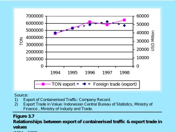
---Figure 3.7
Relationships between export of containerised traffic & export trade in values
(1994 – 1998) Source:
1) Export of Containerised Traffic: Company Record.
2) Export Trade in Value: Indonesian Central Bureau of Statistics, Ministry of Finance , Ministry of Industy and Trade.
By commodity groups, the main export goods from Indonesia are
manufacturing (USD 21.99 billions), which are mainly transported in containers and
primary goods (USD 7.53 billions). It explains why the export of containerised traffic
has strong correlation with export value from Indonesia (see Figure 3.7).
As mentioned earlier in Chapter 2, in the 1960s Indonesia manufactured little
more than handicrafts and a few textiles, but by the mid-1990s Indonesia was
producing manufactured goods that ranged from traditional crafts to aerospace
products. Manufacturing in 1997 accounts for 25 percent of the GDP, up from 13
percent in 1980. Labour-intensive consumer exports, such as footwear and
glassware, in particular have grown quickly.
Indonesia's main manufactured products include food and beverages,
tobacco products, textiles and garments, motor vehicle parts, and electrical
appliances. The main manufactured exports include wood products (veneers,
plywood, and furniture), textiles, clothing, and footwear. All of these products are
transported mainly in containers.
0 1000000 2000000 3000000 4000000 5000000 6000000 7000000
1994 1995 1996 1997 1998
TON
0 10000 20000 30000 40000 50000 60000
USD Million
Container Traffic Forecasting
---Figure 3.8
Relationships between export of containerised traffic & East Asia trade volume growth and trade volume change per annum
(1994 – 1998) Source:
1) Export of Containerised Traffic: Company Record.
2) East Asia Trade Volume Growth and Trade Volume Change per Annum: Ocean Shipping Consultant.
Figure 3.7 shows that the traffic is increasing, but in term of value in USD,
the trend in 1998 was declining. The only reason is the depreciation in value of local
currency (Indonesian Rupiah) to USD where the prices were becoming lower for
export goods.
For East Asian trade volume growth and trade volume change per annum,
there is a negative correlation with export traffic (see Figure 3.8). It seems that when
the East Asian volume growth and trade volume change per annum fell, the export
volume from Indonesia was continually increasing. It can be explained that the
"Asia's export volume increased marginally, as the strong contraction of intra-Asian
trade was only just off-set by a sharp rise in extra-regional flows" (World Bank,
1999). It also shows that probably JICT has performed much better than the other
terminals/ports in the region.
3.4.1.3 Economy sector
Economy is a sector influencing a port beyond the trade sector. The variables
examined from the economy sector are GDP, real GDP growth, average currency
rate and GDP development in Asia. The research identified that there are no strong 0
2000000 4000000 6000000 8000000
1994 1995 1996 1997 1998
TON
-20 -10 0 10 20 30
Percent
TON export
Container Traffic Forecasting
---Figure 3.9
Relationships between export of containerised traffic & real GDP growth of the country and GDP development in Asia
(1994 – 1998) Source:
1) Export of Containerised Traffic: Company Record. 2) Real GDP Growth: Asian Development Bank
3) GDP Development in Asia: Ocean Shipping Consultant.
relationships between the export traffic and those variables. However, real GDP
growth of the country, average currency rate and GDP development in Asia
demonstrate statistical significance (r = -0.61, 0.62, and -0.69 respectively; see
Figures 3.9 and 3.10).
As mentioned in Chapter 2, Indonesia's currency value (Rupiah) sharply
weakened in 1998 with a depreciation of about 71% from the 1997 value following
the economic crisis, which commenced in mid-1997. As the currency rate fell,
Indonesia tried to export as much as possible to increase the GDP of the country.
In addition, between 1991 and 1996, Indonesia experienced the real GDP
growth with an average of 8% but in 1997, due to economic crisis in Asia, the growth
declined (4.9%) and in 1998 the growth was negative (-13.2%). It shows that when
the real GDP growth was lower, Indonesia tried to increase its exports to have
higher GDP by increasing the volume of exports. It also indicates that the demand
is increasing because the importers from foreign countries benefit from lower prices
because of the weakness of the Indonesian currency. They buy products from
Indonesia as ‘cheap’ products.
0 2000000 4000000 6000000 8000000
1994 1995 1996 1997 1998
TON
-15 -10 -5 0 5 10 15
P
e
rcent
TON export
Container Traffic Forecasting
---Figure 3.10
Relationships between export of containerised traffic and the value of local currency rate per USD
(1994 – 1998) Source:
3) Export of Containerised Traffic: Company Record.
4) Currancy rate: Indonesian Central Bureau of Statistics, Bank Indonesia, Ministry of Finance, World Bank, U.S. Department of Commerce (USDOC).
3.4.2 Import traffic
3.4.2.1 Transport sector
Transport is a direct sector influencing a port. The variables examined from the
transport sector are ship calls and container shipping fleet capacity. The research
identified that there is no strong relationship between the import traffic and the
number of ship calls and the development of container shipping fleet capacity (r =
-0.13 and -0.44 respectively; see Figure 3.11).
It may be concluded that there may be no significant effects between the
number of ship calls and the development of container shipping capacity to the
import traffic. It implies that probably the import traffic is influenced by other factors
such as the economy of the country. 0
1000000 2000000 3000000 4000000 5000000 6000000 7000000
1994 1995 1996 1997 1998
TON
0 2,000 4,000 6,000 8,000 10,000 12,000
Rp/
U
S
D
Container Traffic Forecasting
---Figure 3.11
Relationship between import of containerised traffic and fleet capacity and ship calls
(1994 – 1998) Source:
1) Import of Containerised Traffic & Ship calls: Company Record. 2) Fleet Capacity: Ocean Shipping Consultant.
Figure 3.12
Relationships between import of containerised traffic & import trade in value
(1994 – 1998) Source:
1) Import of Containerised Traffic: Company Record.
2) Import Trade in Value: Indonesian Central Bureau of Statistics, Ministry of Finance , Ministry of Industy and Trade.
3.4.2.2. Trade sector
Trade is a sector influencing a port beyond the transport sector. The variables
examined from the transport sector are foreign trade, East Asian trade volume
growth, and trade volume change per annum. The research identified a strong
relationship between the import traffic and the import trade in value (r = 0.97; see
Figure 3.12) and weak relationships with East Asian trade volume growth and trade
volume change per annum (r = -0.39 and 0.42 respectively). It can be said that the
decrease or increase of import traffic reflects the decrease or increase of import
values.
0 2,000,000 4,000,000 6,000,000 8,000,000
1994 1995 1996 1997 1998
TON
0 2000 4000 6000 8000
F
leet
Capacit
y (1000
)
/S
hip Calls
TON Import Fleet capacity Ship calls
0 2,000,000 4,000,000 6,000,000 8,000,000
1994 1995 1996 1997 1998
0 10,000 20,000 30,000 40,000 50,000