Optimization Capabilities of LMS and SMI Algorithm for Smart Antenna Systems (RESEARCH NOTE)

(1)

International Journal of Engineering

J o u r n a l H o m e p a g e : w w w . i j e . i r

Optimization Capabilities of LMS and SMI Algorithm for Smart Antenna Systems

A. Udawat *a_{, P. C. Sharma}b_,_{S. Katiyal}c

a_{Department of Electronics and Communication Engineering, Acropolis Technical Campus, RGPV, India}

b_{Sushila Devi Bansal College of Technology, RGPV, India}

c_{School of Electronics, DAVV, India}

P A P E R I N F O

Paper history:

Received 17 January 2012

Received in revised form 10 September 2012 Accepted 20 June 2013

Keywords:

Smart Antenna Systems SMI

LMS

Angle of Arrival (AOA) Multipath

Array Factor

A B S T R A C T

In the present paper convergence characteristics of Sample Matrix Inversion (SMI) and Least Mean Square (LMS) adaptive beam-forming algorithms (ABFA) are compared for a Smart Antenna System (SAS) in a multipath environment. SAS are employed at base stations for radiating narrow beams at the desired mobile users. The ABFA are incorporated in the digital signal processors for adjusting the weights to adjust the beam on the desired user and generate null in the direction of interferer. SMI and LMS algorithms are used with SAS for improving the performance of wireless communication system by optimizing the radiation pattern according to the signal environment. This can enhance the coverage and capacity of the system in multipath environment by reducing the interference and noise. The data rate can be enhanced by mitigating fading due to cancellation of multipath components. In this paper, optimization capabilities of SMI and LMS are considered by changing the parameters. The results reveal improvement in gain, speed of convergence and reduction in side-lobe level.

doi:10.5829/idosi.ije.2013.26.11b.15

1. INTRODUCTION1

The need for better coverage, increased data rate and enhanced capacity motivated researchers to exploit the SAS and Space Division Multiple Access (SDMA). This can be satisfied by the identification of desired signal from a set of signals available in faded channel. For this ABFA are integrated within SAS with the property of spatial filtering to differentiate between desired user signals and interfering signals [1]. They are capable of reducing noise, increasing signal to noise ratio and enhancing system capacity [2, 3]. The SMI and LMS are the two most widespread non-blind channel equalization techniques based on the principle of calculating the weights (signal amplitude and phase adjustments) according to the variable environment by following specified optimization rules [4, 5]. The signals can be multiplied by a set of weights which are calculated by using objective function inversely related to the quality of signal. These non-lind algorithms use a reference signal for learning the channel information to adjust the weights [6]. The objective of ABFA is minimization of the objective function by reducing the

1*Corresponding Author Email: [email protected] _{(A. Udawat)}

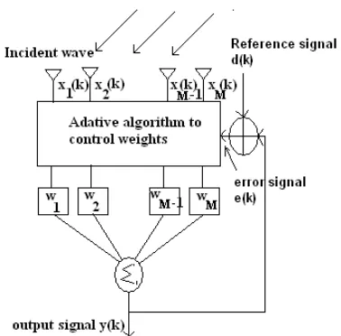
error between a reference signal ( )d k and the array output y k( ). Figure 1 shows the SAS system in which the input signals are multiplied by complex weights

1, 2, , M

w w K w which are adjusted by minimizing a cost function. The reference signal is a training sequence used to train the SAS or a desired signal based upon an a priori knowledge of nature of the arriving signals. When the reference signal is not available, blind optimization techniques are used.

2. PROBLEM FORMULATION

In this paper the comparison of optimization capabilities of SMI and LMS with reference to number of antenna elements and their spacing are presented. Section 3 presents optimization approach of SMI and LMS ABFA with their mathematical description. In Section 4 simulation results using MATLAB 7.0 with reference to number of antenna elements, inter-element distance and angle of arrival (AOA) are obtained to find the optimized values. The array factor plots of SMI and LMS output for the same values of the above-mentioned parameters are presented.

(2)

Figure 1. Adaptive Beam-forming System

3. OPTIMIZATION APPROACH IN LMS AND SMI ABFA

3. 1. LMS Algorithm It is a stochastic version of steepest descent algorithm. The minima for this surface can be established using gradient method by finding the mean square error (MSE).

The convergence of LMS depends on eigen value spread of the covariance matrix and is based on knowledge of the arriving signal [7]. It does not require measurement of correlation functions nor matrix inversion. Most of the non-blind algorithms try to minimize the MSE between the desired signal d k( ) and the array output y k( ). Let y k( ) and d k( ) denote the sampled signal of y t( ) and d t( ) at time instant t_n , respectively. The output response of the uniform linear array given by LMS is [8]

( ) H( ) ( )

y k =w k x k (1)

Then the error signal is given by

( )= ( )- ( )= ( )- H( ) ( )

e k d k y k d k w k x k

The MSE is given by

(2)

2 2

( ) ( ) H( ) ( )

e k = d k -w k x k (3)

wherew defines the weight vector andxis the received signal vector. The cost function is defined as:

2

( ) [ ( ) ]

C k =E e k (4)

whereE[] defines the expectation operator. Combining the above three Equations (2), (3) and (4) we have:

2

( ) ( ) H ( ) H( ) H( ) ( )

C k =E d ké_ë ù_û-p w k -w k p w k Rw k+ (5)

where _{R E x k x k}_{= ë}_é ( ) H( )_ù

û and p E x k d k= ëé ( ) H( )ùû_. Here R is the M ´ M autocorrelation matrix of input vectorx k( ) and pis the M ´1 cross correlation vector between the input data vector

( )

d k .

Solving the above equations using Wiener solution and Steepest descent method optimum weights can be calculated as:

( 1) ( ) ( ( ))

w k+ =w k -mg w k (6)

where (k +1) denotes updated weights computed at (k +1) iterations,m is the step size parameter or weighing constant which can control the size of the incremental correction as we proceed from one step to another. MSE can be obtained by setting the gradient vector of C k( ) equal to 0.

( [ ( )]) 2 2 0

w E e k Rw p

Ñ = - = (7)

The optimum solution for the weight vectorw is given by:

1 opt

w ₌R p

(8)

which is also called the Weiner weight vector [8].

3. 2. SMI Algorithm This method developed by

Reed, Mallet and Brennen [8, 9] is referred [10] as direct matrix inversion which computes the array weights by replacing R with its estimates [10, 11]. The sample matrix is a time average estimate of the array correlation matrix using K - time samples [12]. It is based on an estimate of correlation matrix given by:

1

( ) ( )

K H xx

k

R x k x k K =

=

å

(9)

whereK is the observation interval andxis the signals arrived on antenna array elements, given by:

1 2 3

[ ( ), ( ), ( ),... _M( )]

x= x k x k x k x k (10)

The correlation vector pcan be estimated by:

*

1

( ) ( )

K

k

p d k x k

K =

=

å

(11)

As the weights are adapted block by block and data block is of lengthK , this method can also be termed as block adaptive method. The array correlation matrix and the correlation vector can be calculated by defining matrix as the _kth _{block of}_x_{vectors ranging over}_K

(3)

1 1 1

2 2

(1+ ) (2+ ) ( + )

(1+ ) (2+ )

( )

(1+ ) ( )

K

M M

x kK x kK x K kK x kK x kK

X k

x kK x K + kK

é ù

ê ú

=

ê ú

ë û

L M

M O

L

(12)

Now, the estimate of array correlation matrix is given by:

1

( ) H( )

xx K K

R X k X k

K

= (13)

Also, the desired signal vector can be defined as:

( ) [ (1 ) (2 ) ( )]

d k = d +kK d +kK L d K kK+ (14)

Thus, the estimate of correlation vector is given by:

*

1

( ) ( ) _K( )

p k d k X k K

= (15)

Now, the SMI weights can be calculated for the

th

k block of length K as:

1 1 *

( )₌ -( ) ( ) =[ ( ) H( )]- ( ) ( )

SMI xx K K K

w k R k p k X k X k d k X k ₍₁₆₎

4. SIMULATION RESULTS AND DISCUSSIONS

Simulation of LMS and SMI adaptive algorithm for antenna arrays using M = 5, 8 and 10 elements with inter-element distanced = 0 .5l ,

0 .2 5l _{and 0 .1 2 5}l is performed in MATLAB 7. The step sizem = 0 .0 2 with zero initial weights is considered.

One can define array factor plot as:

2 sin (AF) 2cos

2 d

Array Factor p q

l

æ ö

= _ç _÷

è ø (17)

wheredis the inter-element distance between the antenna elements in terms of wavelength l_,and qis the value of AOA measured with respect to z axis. Here, the desired signal is arriving at an angle of 30° and interferer signal at -60°. The LMS routine is calculated for 100 iterations. The SMI routine is calculated for a block length of

10 0

K = . The value of noise variance is 0.001 in order to keep the inverse of covariance matrix to become singular. The expression for gain in dB used in simulation results is given by:

( )2

41253 20log Gain

q

°

æ ö

ç ÷

= _ç _÷

D

è ø (18)

whereDq is the value of half power beam-width (HPBW), or beam-width in degrees which can be

calculated from the plot using the following expression:

(0.707(AF)) (0.707(AF))

q q+ q

-D = - (19)

Following cases are considered:

4.1. Case I Figure 2 shows the AF plots for LMS with number of elements M = 5, 6, 7, 8, 9 and 10 for 100 iterations ford = 0 .5l . It is clear that LMS generates peak in the desired direction user AOA 30º

and places null in the undesired direction where interferer is located i.e., at -60º. Similarly, AF plots are drawn for different values of d at 0 .3 5l , 0 .2 5l and 0 .1 2 5l in Figures 3, 4 and 5 respectively. The observations drawn from Figures 2, 3, 4 and 5 are indicated in Table 1 in terms of the comparison of beam-width, gain and number of side lobes (SL) for different M and d .

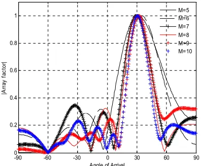
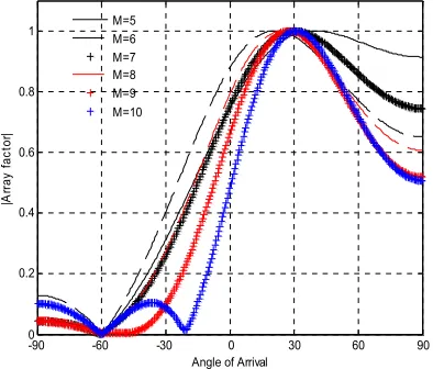
4.2. Case II The AF plot for SMI with M = 5,

6, 7, 8, 9 and 10 for block lengthK =1 0 0are drawn ford =0.5l , 0.35l , 0.25l and 0 .1 2 5l in Figures 6, 7, 8 and 9 respectively. It is evident from these figures that performance of SMI degrades as the value of gain reduces with an increase in beam-width. The observations drawn from Figures 6, 7 ,8 and 9 are indicated in Table 2 in terms of the comparison of beam width, gain and number of side lobes (SL) for different values of M and d .

4.3. Case III The plot of magnitude of array

weights for LMS with M = 5, 6, 7, 8, 9 and 10 for 100 iterations are drawn for d = 0 .5l in Figure 10. It is evident from this figure that performance of LMS is best for M = 8 for

0 .5

d = l .

4.4. Case IV The plot of acquisition and

tracking for LMS with M = 8 is drawn for 100 iterations for d = 0 .5l in Figures 11 and 12 for

0 .0 1

m = and 0 .0 2 , respectively. In Figure 11 convergence took place after 60 iterations, while in Figure 12 convergence is not achieved even after 60 iterations. Thus, it is evident from the two figures that for proper convergence the step-size calculated for eigen-value spread of R (=14.38) must satisfy the condition:

1

0 .0 1 4 (tr a c e R( ))

m £ = .

(4)

Figure 2. AF plot for LMS with user AOA 30° and

interferer AOA at -60°for M =5, 6, 7, 8, 9, 10 and

0 .5 d = l

interferer AOA at -60° for M =5, 6, 7, 8, 9, 10 and

0 .3 5

d = l

0 .2 5

d = l

0 .1 2 5

d = l

Figure 6. AF plot for SMI with user AOA 30° and

0 .5 d = l

0 .3 5

d = l

-90 -60 -30 0 30 60 90

0 0.2 0.4 0.6 0.8 1

Angle of Arrival

|A

rr

ay

F

ac

to

r|

M=5 M=6 M=7 M=8 M=9 M=10

-90 -60 -30 0 30 60 90

0 0.2 0.4 0.6 0.8 1

Angle of Arrival

|A

rr

ay

F

ac

to

r|

M=5 M=6 M=7 M=8 M=9 M=10

-90 -60 -30 0 30 60 90

0 0.2 0.4 0.6 0.8 1

Angle of Arrival

|A

rr

ay

F

ac

to

r|

M=5 M=6 M=7 M=8 M=9 M=10

-90 -60 -30 0 30 60 90

0 0.2 0.4 0.6 0.8 1

Angle of Arrival

|A

rr

ay

F

ac

to

r|

M=5 M=6 M=7 M=8 M=9 M=10

-90 -60 -30 0 30 60 90

0 0.2 0.4 0.6 0.8 1

Angle of Arrival

|A

rr

ay

f

ac

to

r|

M=5 M=6 M=7 M=8 M=9 M=10

-90 -60 -30 0 30 60 90

0 0.2 0.4 0.6 0.8 1

Angle of Arrival

|A

rr

ay

f

ac

to

r|

(5)

interferer AOA at -60° for M = 5, 8, 10 and

0 .2 5

d = l

interferer AOA at -60° for M = 5, 8, 10 and

0 .1 2 5

d = l

Figure 10. Plot of magnitudes of array weights for

LMS with user AOA 30° and interferer AOA at -60°

for M = 5, 8, 10 and d = 0 .5l

Figure 11. Plot of acquisition and tracking of LMS for

0 . 0 1

m =

Figure 12. Plot of acquisition and tracking of LMS for

0 .0 2

m =

Figure 13. Plot of MSE of LMS for M = 5, 6,7, 8, 9

and 10 and d = 0 .5l

-90 -60 -30 0 30 60 90

0 0.2 0.4 0.6 0.8 1

Angle of Arrival

|A

rr

a

y

fa

c

to

r|

M=5 M=6 M=7 M=8 M=9 M=10

-90 -60 -30 0 30 60 90

0 0.2 0.4 0.6 0.8 1

Angle of Arrival

|A

rr

ay

fa

ct

or|

M=5 M=6 M=7 M=8 M=9 M=10

0 10 20 30 40 50 60 70 80 90 100

0 0.05 0.1 0.15 0.2 0.25 0.3 0.35

Iteration no.

|w

ei

gh

ts|

M=5(Black color)

M=6(Blue color) M=7(red color)

M=8(green color)

M=9(yellow color) M=10(magenta color)

0 10 20 30 40 50 60 70 80 90 100

-1.5 -1 -0.5 0 0.5 1 1.5

No. of Iterations

S

ign

a

ls

Desired signal d(k) Array output y(k)

0 10 20 30 40 50 60 70 80 90 100

-1.5 -1 -0.5 0 0.5 1 1.5

No. of Iterations

S

ign

als

Desired signal d(k) Array output y(k)

0 10 20 30 40 50 60 70 80 90 100

0 0.2 0.4 0.6 0.8 1 1.2 1.4 1.6

Iteration no.

M

ean

sq

ua

re

e

rr

or

MSE Plot for LMS for different elements M for d=0.5

(6)

TABLE 1. Comparison of beam-width, gain and number of SL for LMS

No. of Elements (M ) Comparison of Beam-width (in degrees)

0 .5

d = l d =0 .3 5l d =0 .2 5l d =0 .1 2 5l

5 26 37.24 57.25 NA

6 20.63 29.76 41.26 NA

7 17.19 24.70 35.53 94

8 14.90 21.20 30.94 73.29

9 13.17 19.48 26.93 61.40

10 12.60 18.06 23.49 55.67

M Comparison of Gain (in dB)

5 17.85 14.73 10.90 NA

6 19.86 16.68 13.84 NA

7 21.40 18.30 15.14 6.69

8 22.60 19.62 16.34 8.85

9 23.70 20.36 17.54 10.30

10 24.14 21.02 18.73 11.2

M Comparison of Number of SL

5 2 1 2 1

6 5 4 2 0

7 6 4 2 1

8 7 5 3 0

9 8 5 4 1

10 9 6 4 1

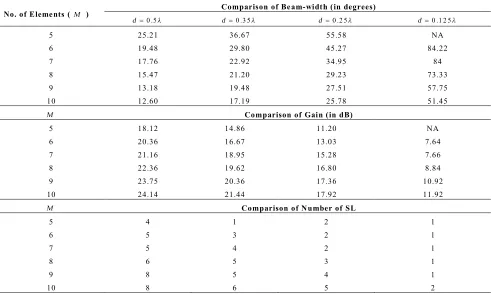
TABLE 2. Comparison of beam-width, gain and number of SL for SMI

No. of Elements (M ) Comparison of Beam-width (in degrees)

0 .5

d = l d =0 .3 5l d =0 .2 5l d =0 .1 2 5l

5 25.21 36.67 55.58 NA

6 19.48 29.80 45.27 84.22

7 17.76 22.92 34.95 84

8 15.47 21.20 29.23 73.33

9 13.18 19.48 27.51 57.75

10 12.60 17.19 25.78 51.45

M Comparison of Gain (in dB)

5 18.12 14.86 11.20 NA

6 20.36 16.67 13.03 7.64

7 21.16 18.95 15.28 7.66

8 22.36 19.62 16.80 8.84

9 23.75 20.36 17.36 10.92

10 24.14 21.44 17.92 11.92

M Comparison of Number of SL

5 4 1 2 1

6 5 3 2 1

7 5 4 2 1

8 6 5 3 1

9 8 5 4 1

(7)

5. CONCLUDING REMARKS

In this paper the optimization capabilities of LMS and SMI are explored and it is found that for d = 0 .5l with M = 8 elements the beam-width of 14.9° is achieved with a gain of 22.60dB for LMS, while a beam-width of 15.47 is achieved with a gain of 22.36dB for SMI. Zero iteration is required for SMI (0.324407 seconds) as compared to 100 iterations for LMS (0.642163 seconds) and thus SMI is faster as compared to LMS. LMS acquires and tracks the desired signal after 60 iterations and the MSE also converges after 60 iterations for m £ 0 .0 1. The slow convergence problem of LMS (1.407494 seconds) for large eigen- spread can be avoided by the use of SMI algorithm (0.291175 seconds). Thus the most suitable performance of antenna arrays using LMS and SMI can be obtained for M = 8 and d = 0 .5l .

6. REFERENCES

1. Yaser, S. and Aleem, M. A., "Performance appraisal of smart antenna systems for next generation wireless communication",

Journal of Engineering and Sciences, Vol. 4, No. 1, (2010),

05-08.

2. Shaukat, S. F., Hassan, M., Farooq, R., Saeed, H. U. and Saleem, Z., "Sequential studies of BFA for SAS", World

Applied Science Journal,, Vol. 6, (2009), 754-758.

3. Rani, C. S., Subbaiah, P., Reddy, K. C. and Rani, S. S., "Lms and rls algorithms for smart antennas in a w-cdma mobile communication environment", ARPN Journal of engineering

and Applied Sciences, Vol. 4, No. 6, (2009), 77-88.

4. Godard, D., "Self-recovering equalization and carrier tracking in two-dimensional data communication systems",

Communications, IEEE Transactions on, Vol. 28, No. 11,

(1980), 1867-1875.

5. Rong, Z., "Simulation of adaptive array algorithms for cdma systems", Virginia Polytechnic Institute and State University. (1996)

6. Stoica, P. and Moses, R. L., "Introduction to spectral analysis", Prentice hall New Jersey:, Vol. 1, (1997).

7. Fares, S. A. and Adachi, F., "Mobile and wireless communications: Physical layer development and implementation", In-The Olajnica, Vukovar, Croatia,, (2010). 8. Godara, L. C., "Applications of antenna arrays to mobile

communications. I. Performance improvement, feasibility, and system considerations", Proceedings of the IEEE, Vol. 85, No. 7, (1997), 1031-1060.

9. Varade, S. W. and Kulat, K., "Robust algorithms for doa estimation and adaptive beamforming for smart antenna application", in Emerging Trends in Engineering and Technology (ICETET), 2nd International Conference on, (2009), 1195-1200.

10. Yasin, M. and Akhtar, P., "Enhanced sample matrix inversion is better meam-former for a smart antenna system", World Applied

Science Journal,, Vol. 10, No. 10, (2010), 1167- 1175.

11. Yan, C., "Smart antenna for wireless communication",

Telecommunications Science, Vol. 5, (2002), 5-10

12. Godara, L. C., Application of antenna arrays to mobile communications, part п: Beam-forming and direction-of-arrival considerations, in Proceeding of the IEEE. (1997), 1195- 1234.

(8)