TRANSONIC TURBULENT FLOW SIMULATION USING
PRESSURE-BASED METHOD AND NORMALIZED VARIABLE
DIAGRAM
M. H. Djavareshkian and S. Baheri Islami
Department of Mechanical Engineering, University of Tabriz Tabriz, Iran, [email protected]
(Received: August 5, 2003 – Accepted in Revised Form: August 18, 2004)
Abstract A pressure-based implicit procedure to solve the Euler and Navier-Stokes equations on a nonorthogonal mesh with collocated finite volume formulation is described. The boundedness criteria for this procedure are determained from Normalized Variable diagram (NVD) scheme. The procedure incorporates the k−ε eddy-viscosity turbulence model. The algorithm is tested for inviscid and turbulent transonic aerodynamic flows around airfoils for different Mach number and angle of attack where the results are compared with other existing numerical solutions for inviscid flow and with experiment and another numerical solution for the turbulent case. The comparisons show that the resolution quality of the NVD scheme is considerable.
Key Words Transonic Flow, Normalized Variable Diagram, SBIC, Pressure-Based, Aerodynamic Coefficients
ﻩﺪﻴﮑﭼ
ﻭﺮـﻠﻳﻭﺍﺕﻻﺩﺎـﻌﻣﻞـﺣﯼﺍﺮﺑﺎﻨﺒﻣﺭﺎﺸﻓﻢﺘﻳﺭﻮﮕﻟﺍﯼﺎﻨﺒﻣﺮﺑﺩﻭﺪﺤﻣﻢﺠﺣﯼﺩﺪﻋﺪﻧﻭﺭﮏﻳﻪﻟﺎﻘﻣﻦﻳﺍﺭﺩﺘﺳﺍﺮﻳﻭﺎﻧ
ﺖـﺳﺍﻩﺪـﺷﺢﻳﺮﺸـﺗﻥﺎﮑﻣﻢﻫﻭﺪﻣﺎﻌﺘﻣﺮﻴﻏﻪﮑﺒﺷﮏﻳﯼﻭﺭﺮﺑﺲﮐﻮ
. ﺪـﻧﻭﺭﺭﺩﯽﮔﺪـﻨﻨﮐﺩﻭﺪﺤﻣﺭﺎـﻴﻌﻣ
ﺪـﺷﺎﺑﯽﻣﻩﺪﺷﺪﻌﺑﯽﺑﯼﺎﻫﺮﻴﻐﺘﻣﻡﺍﺮﮔﺎﻳﺩﮏﻴﻨﮑﺗﯼﺎﻨﺒﻣﺮﺑﺎﻬﻟﻮﻠﺳﺡﻮﻄﺳﺭﺩﻩﺭﺎﺷﻝﺮﺘﻨﮐﯼﺍﺮﺑﻕﻮﻓﯼﺩﺪﻋ
. ﯼﺍﺮـﺑ
ﻝﺪﻣﺯﺍﺲﻧﻻﻮﺑﺭﻮﺗﻪﺘﻳﺯﻮﮑﺴﻳﻭﻥﺩﺮﮐﻝﺪﻣ
ε − k
ﺖﺳﺍﻩﺪﺷﻩﺩﺎﻔﺘﺳﺍ
.
ﺗ
ﺭﺬـﮔﮏﻴﻣﺎﻨﻳﺩﻭﺮﻳﺁﻥﺎﻳﺮﺟ،ﺪﻧﻭﺭﻦﻳﺍﻂﺳﻮ
ﻪﻴﺒـﺷﻪـﻠﻤﺣﻪﻳﻭﺍﺯﯼﺩﺍﺪﻌﺗﻭﺕﻭﺎﻔﺘﻣﺥﺎﻣﺩﺍﺪﻋﺍﯼﺍﺮﺑﯽﮑﻴﻣﺎﻨﻳﺩﻭﺮﻳﺁﻊﻃﺎﻘﻣﯼﻭﺭﺭﺩﺖﺟﺰﻟﻥﻭﺪﺑﻭﻪﺘﻔﺷﺁﯽﺗﻮﺻ
ﺖـﺳﺍﻩﺪـﻳﺩﺮﮔﻪﺴـﻳﺎﻘﻣﯽـﺑﺮﺠﺗﯼﺎـﻫﻩﺩﺍﺩﻭﻩﺪﺷﺮﺸﺘﻨﻣﯼﺩﺪﻋﺞﻳﺎﺘﻧﺎﺑﻩﺪﺷﺝﺍﺮﺨﺘﺳﺍﺞﻳﺎﺘﻧﻭﻩﺪﺷﯼﺯﺎﺳ
. ﻦـﻳﺍ
ﻞﺣﺖﻴﻔﻴﮐﻪﮐﺪﻫﺩﯽﻣﻥﺎﺸﻧﻪﺴﻳﺎﻘﻣ
ﻪـﻈﺣﻼﻣﻞـﺑﺎﻗﺎـﻫﻩﺭﺎﺷﻝﺮﺘﻨﮐﯼﺍﺮﺑﻩﺪﺷﺪﻌﺑﯽﺑﯼﺎﻫﺮﻴﻴﻐﺘﻣﮏﻴﻨﮑﺗﻂﺳﻮﺗ
ﺪﺷﺎﺑﯽﻣ
.
1. INTRODUCTION
Traditionally most transonic flow simulations are carried out by using density-based methods in which density is used as a primary variable in the continuity equation while pressure is extracted from the equation of state. There are a few successful computations obtained from the pressure–based method, which use pressure as the dependent variable, like Zhou & Davidson [1], Zhou et al [2], Patankar [3], Rhie [4], Shyy & Chen [5]. The advantage of the pressure-based schemes is that they are efficient for both compressible and incompressible flows, therefore they are often argued to be an algorithm for all speed flows. Almost all of the pressure-based
methods use a dissipation model, which applies an artificial dissipation to prevent the unphysical behavior. An important problem in discretization of flow equations is estimating of convective terms on cell faces using neighboring nodes. High order schemes tend to provoke oscillations in the solution when the local Peclet number is high in combination with steep gradients of the flow properties. To suppress oscillations associated with higher–order schemes, many techniques have been advertised.
MUSCL (Van Leer [7]) type of TVD Scheme into their pressure-based procedure; the flux limiter in their work relies on the gradients of the solved dependent variable. There is also the work of Shyy and Thakur [8] who developed what they call the controlled variation scheme (CVS), which is based on the formalism of the TVD concept. Their CVS scheme was generalized to compressible flows containing shocks as well as incompressible flows by Thakur et al. [9]. Issa and Javareshkian [10] implemented a high resolution TVD scheme with characteristic-variable-based flux limiters into a pressure-based finite volume method. Kobayashi and Pereira [11] and Batten et al. [12] where characteristic-based flux computations were introduced into pressure-correction solution procedures. Kobayashi and Pereira use the essentially nonoscillating scheme for the flux calculation. Leonard [13] has generalized the formulation of the high–resolution flux limiter schemes using what is called the normalized variable formulation (NVF). The NVF methodology has provided a good framework for development of high – resolution schemes that combine simplicity of implementation with high accuracy and boundedness. Most of NVD methods use different differencing schemes through the solution domain. This procedure includes some kind of switching between the differencing schemes.
Switching introduces additional instability into the computation. The worst case is that instead of a single solution for steady state problem, the differencing scheme creates two or more unconverged solution with the cyclic switching between them. In that case it is impossible to obtain a converged solution and the convergence stalls at some level. Javareshkian [14] has recently developed the Second and Blending Interpolation Combine (SBIC) scheme with the minimum number of adjustable parameters in the pressure based algorithm. One advantage of this scheme in comparison with all other differencing NVD schemes is some kind of switching only two differencing schemes, central differencing and blending between upwind and central differencing are included that blending factor is determined automatically. Another advantage of this scheme in comparison with TVD and ENO schemes is the simplicity of implementation with high accuracy
and boundedness. This scheme has been used to the computation of steady subsonic, transonic and supersonic internal as well as to the transient problem [14]. Djavareshkian and Baheri Islami [15] developed this scheme for simulation of flow around the airfoil.
The contribution of the present paper is to extend this scheme and apply it to new cases for which the results are compared against available experimental data and other numerical solutions; these include transonic turbulent airfoil flow simulation and the calculaiton of the aerodynamic coefficients for many inviscid/turbulent test cases.
2. GOVERNING EQUATIONS
The basic equations, which describe conservation of mass, momentum and scalar quantities, can be expressed in Cartesian tensor form as
0 x
) u (
t j
j =
∂ ρ ∂ + ∂
ρ
∂ (1)
u i j
ij j i
i S
x ) T u u (
t ) u
( =
∂ − ρ ∂ + ∂ ρ
∂ (2)
φ
= ∂
− φ ρ ∂ + ∂
φ ρ ∂
S x
) q u (
t ) (
j j
j (3)
The stress tensor and scalar flux vector are usually expressed in terms of basic dependent variable. The stress tensor for a Newtonian fluid is
) x u
x u ( x
u 3 2 p T
i j j i ij
k k ij
ij ∂
∂ + ∂ ∂ µ + δ ∂
∂ µ − δ −
= (4)
The scalar flux vector usually given by the Fourier-type law:
) x ( q
j
j ∂
φ ∂ Γ
= φ (5)
Turbulence is accounted for by adopting the
ε −
diff comp j k j j D G ) x k k u ( x ) k ( t Θ + + ε ρ − = ∂ ∂ Γ − ρ ∂ ∂ + ρ ∂ ∂ (6) k C G k C ) x u ( x ) ( t 2 2 1 j j j ε ρ − ε = ∂ ε ∂ Γ − ε ρ ∂ ∂ + ε ρ ∂ ∂
ε (7)
The turbulent viscosity and diffusivity coefficients are defined by
ε ρ =
µt Cµ k2 (8)
) ( tt
t
φ φ= σµ
Γ (9)
and the generation term G in Equations 6 and 7 is defined by ⎥ ⎥ ⎦ ⎤ ⎢ ⎢ ⎣ ⎡ ∂ ∂ ⎟⎟ ⎠ ⎞ ⎜⎜ ⎝ ⎛ ρ + ∂ ∂ δ − ∂ ∂ ⎟ ⎟ ⎠ ⎞ ⎜ ⎜ ⎝ ⎛ ∂ ∂ + ∂ ∂ µ = j i m m ij j i i j j i t x u k x u 3 2 x u x u x u
G (10)
The terms Dcomp and Θdiff are additional contributions to the standard k−ε model often introduced to account for the effects of compressibility [16]. In this work, the models proposed by Yang et al. [16] are adopted, namely,
i i t i i comp x p x . . 1 x u k 55 9 D ∂ ∂ ∂ ρ ∂ ρ µ ρ − ∂ ∂ ρ −
= (11)
0
diff =
Θ (12)
The latter being appropriate for high-Reynolds-number flows, as is the case here. The values of the turbulence model coefficients used in the present work are given in Table 1.
3. DISCRETIZATION
The discretization of the above differential
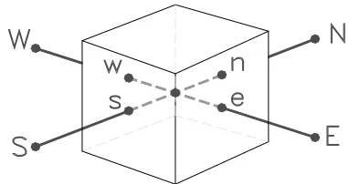
equations is carried out using a finite-volume approach. First, the solution domain is divided into a finite number of discrete volumes or cells, where all variables are stored at their geometric centers (see e.g. Figure 1). The equations are then integrated over all the control volumes by using the Gaussian theorem. The discrete expressions are presented affected with reference to only one face of the control volume, namely, e , for the sake of brevity.
For any variable φ (which may also stand for the velocity components), the result of the integration yields υ δ = − + − + φ ρ − φ ρ δ υ δ φ + S I I I I ] ) ( ) [(
t e w n s
n p 1
n
p (13)
where I ’s are the combined cell-face convection c
I and diffusion I fluxes. The diffusion flux is D approximated by central differences and can be written for cell-face e of the control volume in Figure 1 as:
φ
− φ − φ
= e p E e
D
e D ( ) S
I (14)
where S stands for cross derivative arising from φe mesh nonorthogonality. The discretization of the convective flux, however, requires special attention and is the subject of the various schemes developed. A representation of the convective flux for cell-face e is:
e e e e c
e ( .V. ) F
I = ρ Α φ = φ (15)
TABLE 1. Values of Empirical Coefficients in the Standard k−ε Turbulence Model.
1
C C2 Cµ σk σε
1.44 1.92 0.09 1.0 1.3
the value of φe is not known and should be estimated by interpolation, from the values at neighboring grid points. The expression for the φe is determined by the SBIC scheme, that is based on the NVD technique, used for interpolation from the nodes E, P and W. The expression can be written as
e W E W
e
φ
φ
φ
φ
φ
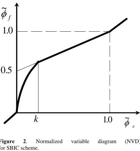
= +( − ).~ (16)the functional relationship used in SBIC [14] scheme for ~φe is illustrated in Figure 2 and is given by:
P e
~ ~ = φ
φ if ~φC∉
[ ]
0,1P P e P 2 P P e P e ~ ) 1 x ~ ( K x ~ x ~ 1 ~ ) 1 x ~ ( K x ~ x ~ ~ φ ⎟⎟ ⎠ ⎞ ⎜⎜ ⎝ ⎛ − − + + φ − − − = φ
if ~φP∈
[ ]
0,KP P e P e P e ~ 1 x ~ 1 x ~ 1 x ~ x ~ x ~ ~ φ − − + − − = φ
if ~φP∈
[ ]
0,K 0≤K ≤0.5 (17)where W E W P P W E W e e W E W e e W E W P P x x x x x ~ x x x x x ~ ~ ~ − − = − − = φ − φ φ − φ = φ φ − φ φ − φ = φ
the limits on the selection of K could be determined in the following way. Obviously the lower limit is K=0, which would represent switching between upwind and central differencing. This is not favorable because; it is essential to avoid the abrupt switching between the schemes in order to achieve the converged solution. The value of K should be kept as low as possible in order to achieve the maximum resolution of the scheme.
With higher-order schemes, the evaluation of e
φ may involve a large number of neighboring grid points. Therefore, in order to simplify the solution of the resulting system of algebraic equations, a compacting procedure is usually used. The deferred correction procedure of Rubin and Khosla [17] adapted in this work, is based on replacing the convective flux at control volume face by an equivalent flux given by
) (
F F F
Iec = eφe = eφeU− e φeU−φe
where the superscript U denotes values obtained by the first-order upwind scheme, and φe represents cell face value computed by SBIC scheme. With the preceding assumption, each discretized equation contains five unknowns (in two dimensions), and the matrix of coefficients of the resulting system of equations is pentadiagonal and always diagonally dominates since it is formed using the first order upwind scheme. The final form of the discretized equation from each approximation is given as:
dc S , N , W , E m m m P
P. A . S S
A φ =
∑
φ + ′ += φ
(18)
where 'A s are the convection-diffusion coefficients. The term S'φ in Equation 18 contains quantities arising from non-orthogonality, numerical dissipation terms and external sources, and
P ) t /
(ρδυ δ φ of the old time-step/iteration level (for time dependent equation). For the momentum equations it is easy to separate out the pressure-gradient source from the convected momentum
~
φ
f~
φ
c1 0
.
1 0
.
0 5
.
k
fluxes. S is the contribution due to the adapted dc deferred correction procedure.
4. SOLUTION ALGORITHM
The set of Equation 18 is solved for the primitive variable (velocity components and energy) together with continuity utilizing pressure-based implicit sequential solution methods. The technique used is the SIMPLE scheme presented herein. In this technique, the methodology has to be adapted to handle the way in which the fluxes are computed in Equations 15-17. The adapted SIMPLE scheme consists of a predictor and corrector sequence of steps at every iteration. The predictor step solves the implicit momentum equation using the old pressure field. Thus, for example, for the u component, the momentum predictor stage can be written as ' u o * * S p D ) u ( H
u = − ∇ + (19)
where H contains all terms relating to the surrounding nodes and superscripts * and o denote intermediate and previous iteration values, respectively. Note that the pressure-gradient term is now written out explicitly; it is extruded from the total momentum flux by simple subtraction and addition. The corrector-step equation can be written as ' u * * *
* H(u ) D p S
u = − ∇ + (20)
Hence, from Equations 19 and 20
p D u or ) p p ( D u
u** * ** *
δ ∇ − = δ − ∇ − = − (21)
Now the continuity equation demands that
0 ) u (ρ* ** =
∇ (22)
for steady-state flows. For compressible flows it is essential to account for the effect of change of density on the mass flux as the pressure changes.
This is accounted for by linearizing the mass fluxes as flows [18]
u u u u
u** o * o * * ≈ρ +ρ δ + δ
ρ (23)
or p ) dp d ( u p D u
u** o * o *
* ≈ρ −ρ ∇δ + ρ δ
ρ (24)
where Equation 21 is invoked to eliminate uδ , and
δρ is related to pδ by the appropriate equation of state. Substitution of Equation 24 into Equation 22 yields a pressure-correction equation of the form
P * S S * N N * W W * E E * P P S p . A p . A p . A p . A p . A + δ + δ + δ + δ = δ (25)
where S is the finite difference analog of P )
u (ρo *
∇ , which vanishes when the solution is converged. The A coefficients in Equation 25 take the form (the expression for A is given as an E example) e e * e e o E ) dp d .( ) u a ~ ( ) D a ~ (
A = ρ −λ ρ (26)
where λ is a factor whose significance is explained subsequently. The mass flux at a cell face is computed from nodal values of density and velocity, the cell-face values of ρoeand u in *e Equation 26 are not readily available. To compute those values, assumptions concerning the variations of ρ need to be made. In upwinding λ=1 when u is positive; otherwise it would be zero. Alternatively, in central difference formula λ=1/2. Such assumptions have no influence whatsoever on the final solution because they affect only the pressure-correction coefficients, and as pδ goes to zero at convergence, the solution is, therefore, independent of how those coefficients are formulated; however, they do influence the convergence behavior [19].
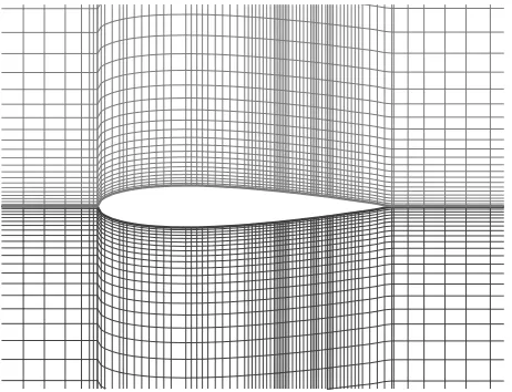
Figure 3. Part of the grid used for the NACA 0012 airfoil.
simulates the hyperbolic nature of the equation system. Indeed, a closer inspection of expression (26) would reveal an upstream bias of the coefficients ( A decreases as u increases), and this bias is proportional to the square of the Mach number. Also note that the coefficients reduce identically to their incompressible form in the limit of zero Mach number.
The overall solution procedure follows the same steps as in the standard SIMPLE algorithm, with the exception of solving the hyperbolic-like pressure-correction (25). To ensure convergence of the iteration process, under relaxation factors between 0.1 and 0.2 for pressure correction and between 0.2 and 0.5 for the other variables are employed.
5. BOUNDARY CONDITIONS
At the inlet, only three of the four variable need to be prescribed: the total temperature, the angle of attack, and the total pressure. The pressure is obtained by zeroth order extrapolation from interior points. At outlet, the pressure is fixed when the outlet is subsonic. Slip boundary conditions are used for far field. Slip boundary conditions are also used on the lower and upper walls of the airfoil in the inviscid flow test cases. In the case of viscous
flow, the non-slip condition is applied at the solid surfaces. To account for the steep variations in turbulent boundary layers near solid walls, wall functions, which define the velocity profile in the vicinity of no-slip boundaries, are employed [20].
6. RESULTS
6.1. Inviscid Part
In the first part, the inviscid flow calculations are presented and the second part turbulent flow is considered. Computational results are shown in several figures for a baseline series of test cases. The results are compared with existing numerical or experimental solutions obtained by others. In this paper H grid is used (Figure 3). Grid independence studies were performed for inviscid cases on grids of 116×149, 150×149 and 301×155 [21]. The far-field boundary placed at 17 chord lengths away from the airfoil surface and 20 chord lengths away from the leading and trailing edges. The value of K in SBIC method for all cases is 0.4.The first case which considered is transonic flow around an NACA 0012 airfoil at M∞=0.85,
α=0º and a 116×149 grid. The distribution of pressure coefficient on the upper and lower surfaces of airfoil are shown in Figure 4. The results are compared with those of presented in
-1.5
-1
-0.5
0
0.5
1
1.5
0 0.2 0.4 0.6 0.8 1
X/C Cp
SBIC
Jameson
[22]. It can be seen that the computed results show good agreement. A sharp discontinuity is achieved successfully for both shock strength and location. Also aerodynamic coefficients for this case are presented in Table 2. Accuracy of these coefficients is good.
The second case is transonic flow around NACA0012 airfoil at M∞=0.85, α = 1º and a 150
×
149 grid. For this case distribution ofpressure coefficient on the upper and lower surface of airfoil are shown in Figure 5. The results are compared with those of Zhou and Davidson [23]. The results of the SBIC scheme show that the upper and lower surface shocks are captured well. Aerodynamic coefficients are presented in Table 3 and compared with available results. Agreement between results is presented.
Third case is for M∞=0.8, α = 1.25º and a 150
×
149 grid. The distribution of pressure coefficient on the upper and lower surfaces of airfoil are shown in Figure 6. It can be seen that TABLE 2. Aerodynamic coefficients NACA0012: M = 0.85,α = 0.
CM CD
CL Method
0 0.0471 0
Rizzi [22]
0 0.0559 0
Zhou & Davidson [23]
0 0.049
0 Current Method
TABLE 3. Aerodynamic Coefficients NACA0012: M = 0.85, α = 1.
CM CD
CL Method
-0.1393 0.0604
0.3938 Pulliam [30]
-0.1282 0.0662
0.3890 Zhou & Davidson [23]
- 0.0418 0.3520
Dervieux & Debiez [31]
- 0.0582 0.3861
Jameson & Martinelli [32]
-0.119 0.0584
0.331 Present Method
TABLE 4. Aerodynamic Coefficients NACA0012 M = 0.8,
α= 1.25.
CM CD
CL Method
-0.0377 0.023
0.3513 Rizzi [22]
-0.0432 0.0237
0.3695 Caughey [33]
-0.0411 0.0236
0.3618 Pulliam [30]
-0.0375 0.022
0.3575 Zhou & Davidson [23]
- 0.0232 0.3654
Jameson & Martinelli [32]
0.04123 0.0248
0.334559 Present Method
-1.5
-1
-0.5
0
0.5
1
1.5
0 0.2 0.4 0.6 0.8 1
X/C
Cp
SBIC (Upper Surface) SBIC (Lower Surface) Zhu
Figure 5. Surface pressure coefficient distribution α= 1 and M = 0.85.
-1.5
-1
-0.5
0
0.5
1
1.5
0 0.2 0.4 0.6 0.8 1
X/C
Cp
SBIC (Upper Surface) SBIC (Lower Surface) Anderson
these results (especially shock gradients) are nearly the same for two methods. In this case, results are compared with those of Anderson and James [24]. Comparison between aerodynamic coefficients is performed in Table 4.
6.2. Viscous Part
For turbulent flow, the k−εturbulence model has been used. Grid independence studies were performed for these cases on grids of 301×155, 494×153, 544×153 and 700×250 [21]. The first case is transonic flow around NACA 0012 airfoil at M∞=0.7, α=1.49º, Re∞=9×10⁶
and a 494×153 grid. 762 nodes are located on the total surface of the airfoil. Distribution of pressure coefficient, contours of pressure coefficient and Mach number are shown in Figures 7(a), 7(b) and 7(c). The results are compared with those of Harris [25]. Aerodynamic coefficients are compared with those of presented in [26]. Agreement between contours and lift coefficient is very good.
Another case is turbulent flow around an RAE 2822 airfoil at M∞=0.734, α = 2.54º,
6
10 5 . 6
Re∞ = × and a 544×153 grid. 728 nodes
are located on the total surface of the airfoil.
-1.5
-1
-0.5
0
0.5
1
1.5
0 0.2 0.4 0.6 0.8 1
X/C
Cp
SBIC (Upper Surface) SBIC (Lower Surface) Harris
(a) (b)
(c)
-1.5
-1
-0.5
0
0.5
1
1.5
0 0.2 0.4 0.6 0.8 1
X/C
Cp
SBIC (Upper Surface) SBIC (Lower Surface) Cook
(a)
(b) (c)
5000 10000
X
10-5
10-4
10-3
10-2
K
-E
q.
Eps
il
on
-Eq.
E
ne
rg
y-E
q. K-Eq.Epsilon-Eq.
Energy Eq.
(c) (d)
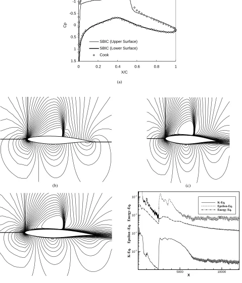
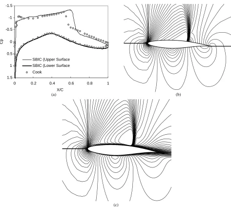
Figure 8. (a) Surface pressure coefficient distribution α= 2.54 and M = 0.734, CL = 0.7513 (SBIC), CL = 0.794 (Hellström); (b) Pressure coefficient contours α= 2.54 and M = 0.734; (c) Much number contours α= 2.54 and M = 0.734;
Related figures for this case are 8(a), 8(b) and 8(c). Pressure coefficient distribution is compared with experimental results of Cook et al., which is resented in [27]. Aerodynamic coefficients are compared with those of Hellstro&&m and Davidson [28]. Convergence histories for the six equations are shown in Figure 8(d). In the start of the running, the value of K in SBIC scheme is chosen with high value, 0.8, for better convergence, after much iteration, in order to achieve the maximum resolution of the scheme, K is changed from 0.8 to 0.4. As you can see, when the K is changed after
2400 iteration, the convergence histories are suddenly changed.
Third case is turbulent flow around an RAE 2822 airfoil at M∞=0.754, α=2.57º and 6
10 5 . 6 Re∞ = × .
Grid, number of nodes and comparison reference are similar to previous case. Distribution of pressure coefficient, contours of pressure coefficient and Mach number are shown in Figures 9(a), 9(b) and 9(c). It is obvious from Figure 9(a) that the shock location is predicted too late, because the flow separates at the shock. The amount of separation and the position of the shock are very dependent -1.5
-1
-0.5
0
0.5
1
1.5
0 0.2 0.4 0.6 0.8 1 X/C
Cp
SBIC (Upper Surface SBIC (Lower Surface Cook
(a) (b)
(c)
on the turbulence model used [28,29]. The influence of turbulence models on lift and drag coefficients are presented in Table 5 [28]. Agreement between aerodynamic coefficient of present study and those of Table 5, which obtained by k−ε turbulence model, is considerable.
7. CONCLUSION
A pressure–based implicit procedure has been described, that incorporates a new NVD scheme. The SBIC scheme is applied to calculate external inviscid and turbulent transonic flow and the results are compared with experiment and other existing numerical solutions. This scheme is able to accurately predict the shock locations and aerodynamic coefficients. The main findings can be summarized as follows:
1. The agreement between the results of the SBIC scheme with experimental and other numerical results is excellent.
2. The simplicity of implementation is one of the advantages of the SBIC scheme.
3. The grid dependence test of the inviscid test case indicates that an acceptable solution can be obtained even on fairly coarse meshes, verifying the practicability of the method for engineering applications.
4. Application of the method to turbulent flow
validates the implementation in frictional flow. 5. Since the flow separates at the shock, the
shock location for turbulent flow is predicted too late by k−ε turbulent model.
8. NOMENCLATURE
D ,
A = finite difference coefficients a
~ = cell face area 2
1,C C ,
Cµ = empirical coefficients
F = mass flux
I = flux
k = kinetic energy of turbulence
K = a factor in SBIC scheme to determine a special scheme
∞
M = a free stream Mach number q = scalar flux vector
∞
R = a free stream Reynolds number T = stress tensor
v ,
u = mean (time-average) velocity components in x and y directions, respectively
α = angle of attack
Γ = diffusivity coefficient
t
Γ
= turbulent diffusivity coefficientδυ = cell volume
ε = volumetric rate of dissipation
µ = dynamic viscosity t
µ = turbulent viscosity
ρ = density
k
σ = turbulent prandtl number for turbulent kinetic energy
ε
σ = turbulent prandtl number for dissipation rate
φ = scalar quantity
φ
~
= normalized scalar quantity
8. REFERENCES
1. Zhou, G. and Davidson, L., “A Pressure-Based Euler Scheme for Transonic Internal and External Flow Simulation”, Journal of Computational Fluid Dynamics, Vol. 5, (1995), 169-188.
2. Zhou, G., Davidson, L. and Olsson, E., “Shock Capturing
TABLE 5. The Influences of Turbulence Models on Lift and Drag Coefficients. RAE 2822 : M=0.754, α=2.57○.
CD CL
Turbulence Model
0.0262 0.716
RSM [28]
0.0270 0.731
RSM-GGDH [28]
0.0297 0.783
k−ε [28]
0.02975 0.784
Present
0.0284 0.789
Baldwin-Lomax [28]
0.0239 0.735
for Supersonic Flow Using a Pressure Algorithm with Semi-Retarded Density, Numerical Methods in Laminar and Turbulent Flow”, Vol. 1X, Part 1, Pineridge Press, Swansea, UK, (1995), 505-515.
3. Patankar, S. V., “Numerical Heat Transfer and Fluid Flow”, McGraw–Hill, Washington, (1980).
4. Rhie, C. M., “A Pressure Based Navier-Stokes Solver Using the Multigrid Method”, AIAA Paper, 86-0207, (1986).
5. Shyy, W. and Chen, M. H., “Pressure – Based Multigrid Algorithm for Flow at All Speeds”, AIAA Journal, Vol. 30, No. 11, (1992),2660 – 2669.
6. Lien, F. S. and Leshziner, M. A., “A Pressure-Velocity Solution Strategy for Compressible Flow and Its Application to Shock Boundary-Layer Interaction Using Second-Moment Turbulence Closure”, Journal of Fluids Engineering, Vol. 115, No. 4, (1993), 717-725.
7. Van Leer, B., “Towards the Ultimate Conservative Difference Scheme. II. Monotonicity and Conservation Combined in Second Order Scheme”, Journal of Computational Physics, Vol. 14, No. 4, (1974), 361-370. 8. Shyy, W., and Thakur, S., “Controlled Variation Scheme
in a Sequential Solver for Recirculating Flow”, Heat Transfer, Vol. 25, No. 3, Pt. B, (1994), 273-286.
9. Thukur, S., Wright, J., Shyy, W., Liu, J., Ouyang, H., and Vu, T., “Development of Pressure-Based Composite Multigrid Methods for Complex Fluid Flows”, Progress in Aerospace Sciences, Vol. 32, No. 4, (1996), 313-375. 10. Issa, R. I. and Javareshkian, M. H., “Application of TVD
Scheme in Pressure-Based Finite-Volume Methods”,
Proceedings of the Fluids Engineering Division Summer Meeting, Vol. 3, American Society of Mechanical Engineering, New York, (1996), 159-164. 11. Kobyashi, M. H. and Pereira, J. C. F.,
“Characteristic-Based Pressure Correction at all Speed”, AIAA Journal, Vol. 34, No. 2, (1996), 272-280.
12. Batten, P., Lien, F. S. and Leschziner, M. A., “A Positivity-Preserving Pressure-Correction Method”,
Proceedings of 15th International Conf. On Numerical Methods in Fluid Dynamics, Monterey, CA, (1996). 13. Leonard, B. P., “Simple High – Accuracy Resolution
Program for Convective Modeling of Discontinuities”,
Int. J. Num. Meth. Eng., Vol. 8, (1988), 1291 – 1318. 14. Javareshkian, M. H., “A New Control Scheme for
Convective Part of Transport Equations Based on Normalized Variable Diagram in Pressure”, Based Methods Proceedings of the 4th International & 8th Annual Conference of Iranian Society of Mechanical Engineers, Vol. 2, (2000), 983 – 989.
15. Djavareshkian, M. H. and Baheri Islami, S., “Aerodynamic Flow Simulation Using Pressure-Based Method And Normalized Variable Diagram”,
Proceedings of 2002 ASME, Computers and Information in Engineering Conference 22nd, Montreal, Canada, (September 29 to October 2, 2002). 16. Yang, Z. Y., Chin, S. B. and Swithenbank, J., “On the
Modeling of the k-Equation for compressible Flow”, 7th International Symposium on Numerical Methods in Laminar and Turbulent Flow, Stanford, CA, (July 1991).
17. Rubin, S. G. and Khosla, P. K., “Polynomial Interpolation
Method for Viscous Flow Calculations”, J. Comput. Phys., Vol.27, (1982), 153-168.
18. Karki, K. C. and Patankar, S. V., “Pressure-Based Calculation Procedure for Viscous flows at All Speeds in Arbitrary Configurations”, AIAA Journal, Vol. 27, No. 9, (1989), 1167-1174.
19. Issa, R. I. and Javareshkian M. H., “Compressible Inviscid and Turbulent Flow Calculation Using a Pressure-Based Method with a TVD Scheme”, AIAA Journal, Vol. 36, No. 9, (1988), 1652-1657.
20. Launder, B. E. and Spalding, D. B., “The Numerical Computation of Turbulent Flows”, Computer Methods in Applied Mechanics and Engineering, Vol. 3., (1974), 269.
21. Baheri Islami, S., “Airfoil Flow Simulation Using Pressure-Based Method and Normalized Variable Diagram”, MSc. Thesis, Dept. of Mech. Engg., Tabriz University, Iran, (2002).
22. Rizzi, A., “Spurious Entropy and Very Accurate Solutions to Euler Equations”, AIAA Paper, (1984), 84-1644.
23. Zhou, G. and Davidson, L., “A Pressure Based Euler Scheme for Transonic Internal and External Flow Simulation”, Int. J. Comput. Fluid Dynamics, Vol. 5, No. 3-4, (1995), 169-188.
24. Anderson, W. K. and James, L. T., “Comparison of Finite Volume Flux Vector Splitting for the Euler Equations”, AIAA J., Vol. 24, No. 9, (1986), 1453-1460. 25. Harris, C., “Two Dimensional Aerodynamic Characteristics
of the NACA0012 Airfoil in the Langley 8-Foot Transonic Pressure Tunel”, ASA Tech. Rep., TM 81927, (1981). 26. Anderson, W. K. and Bonhous, D. L., “An Implicit
Upwind Algorithm for Computing Turbulent Flows on Unstructured Grids”, Computers Fluids, Vol. 23, No.1, (1994), 1-21.
27. Cook, P. H., McDonald, M. A. and Firmin, M. C. P., “Aerofoil RAE 2822-Pressure Distributions and Boundary Layer and Wake Measurements”, AGARD Advisory Report, 138, (1994).
28. Hellström, T. and Davidson, L., “Reynolds Stress Transport Modeling of Transonic Flow Around the RAE2822 Airfoil”, 32nd Aerospace Sciences Meeting,
AIAA paper, No. 94-0309, (1994).
29. Lien, F. S., Kalitzin, G. and Durbin, P. A., “RANS Modeling for Compressible and Transitional Flows”,
Proceedings of the Summer Program, Center for Turbulence Research, (1998), 267-286.
30. Pulliam, T. H. and Barton, J. T., “Euler Computations of AGARD Working 07 Airfoil Test Cases”, AIAA Paper, (1985), 85-0018.
31. Dervieux, A. and Debiez, C., “Application of Mixed Element-Volume Muscl Method with 6th Order Viscosity Stabilization to Steady and unsteady Flow Calculation”,
Proceeding of Computational Fluid Dynamics, John Wiley & Sons Ltd, (1996).
32. Jameson, A. and Martinelli, L., “Mesh Refinement and Modeling Errors in Flow Simulation”, AIAA J., Vol. 36, No. 5, (1998).