R
EGULARA
RTICLEDevelopment of a control-oriented power plant simulator
for the molten salt fast reactor
Claudio Tripodo, Andrea Di Ronco, Stefano Lorenzi, and Antonio Cammi*
Politecnico di Milano, Department of Energy, Nuclear Engineering Division, Via La Masa 34, 20156 Milan, Italy
Received: 9 April 2019 / Received infinal form: 27 July 2019 / Accepted: 26 August 2019
Abstract.In this paper, modelling and simulation of a control-oriented plant-dynamics tool for the molten salt fast reactor (MSFR) is presented. The objective was to develop a simulation tool aimed at investigating the plant response to standard control transients, in order to support the system designfinalization and the definition of control strategies. The simulator was developed employing the well tested,flexible and open-source object-oriented Modelica language. A one-dimensional modelling approach was used for thermal-hydraulics and heat transfer. Standard and validated thermal-hydraulic Modelica libraries were employed for various plant components (tubes, pumps, turbines, etc.). An effort was spent in developing a new MSR library modelling the 1D flow of a liquid nuclear fuel, including an ad-hoc neutron-kinetics model which properly takes into consideration the motion of the Delayed Neutron Precursors along the fuel circuit and the consequent reactivity insertion due to the variation of the effective delayed fractions. An analytical steady-state 2-D model of the core and the fuel circuit was developed using MATLAB in order to validate the Decay Neutron Precursors model implemented in the plant simulator. The plant simulator was then employed to investigate the plant dynamics in response to three transients (variation of fuelflow rate, intermediateflow rate and turbine gasflow rate) that are relevant to control purposes. Simulation outcomes highlight the typicalreactor-follows-turbinebehavior of the MSFR, and they show the small influence of fuel and intermediateflow rate on the reactor power and their strong effects on the temperatures in their respective circuits. Starting from the insights on the reactor behavior gained from the analysis of its free dynamics, the plant simulator here developed will provide a valuable tool in support to thefinalization of the design phase, the definition of control strategies and the identification of controlled operational procedures for reactor startup and shutdown.
1 Introduction
The objective of this work was to develop a fast-running, control-oriented plant-dynamics simulation tool for the molten salt fast reactor (MSFR) and the associated Balance of Plant, and to use it to investigate and analyze the plant dynamics.
The MSFR is the circulating-fuel fast-neutron-spec-trum reactor concept currently object of research under the EU SAMOFAR project (http://samofar.eu/), within the international framework for the development of fourth-generation nuclear reactors known as Generation-IV International Forum [1]. The demonstration of the load-following capabilities and the control operability of the reactor is one of the objectives of the SAMOFAR project. In this view, it is important to rely on a power plant simulator to study the system dynamics and to develop and test the control strategies. Due to the dynamic and control
related purposes of the power plant simulator, an object-oriented modelling approach is selected as suitable choice for the model-based control design. Due to its features in terms of hierarchical structure, abstraction and encapsu-lation, this approach allows developing a model that satisfies the requirements of modularity, openness and efficiency [2]. A viable path to achieve the above-mentioned goals is constituted by the adoption of the Modelica language [3]. Modelica is an object-oriented, declarative, equation-based language developed for the component-oriented modelling of complex physical and engineering systems [2]. It allows a description of single system components (or objects) directly in terms of physical equations and principles, and to connect different compo-nents through standardized interfaces (or connectors). In addition, his acausal component-based modelling strategy provides high reusability of the models andflexibility of the plant configuration, as well as a more realistic description of the plant, since several validated libraries of power plant components exist (e.g. the ThermoPower library [4]). Modelica is open-source and it has already been * e-mail:[email protected]
©C. Tripodo et al., published byEDP Sciences, 2019
https://doi.org/10.1051/epjn/2019029 & Technologies
Available online at: https://www.epj-n.org
successfully adopted in differentfields, such as automotive, robotics, thermo-hydraulic and mechatronic systems, but also in nuclear simulation field. Plant simulators were developed for control purposes for the ALFRED (Advanced Lead Fast Reactor European Demonstrator) reactor [5] and the IRIS reactor [6]. As simulation environment, Dymola (Dynamic Modelling Laboratory) [7] was adopted, even if open-source implementation can be considered as alternative option, e.g. OpenModelica [8].
In developing the power plant simulator for the MSFR, it is essential to consider the peculiar features of this reactor,firstly the presence of a liquid circulating nuclear fuel that acts contemporarily as coolant. The strong physical coupling of thermo-fluid-dynamics and neutronics which characterizes the MSFR indeed required to take into account the motion of the Delayed Neutron Precursors (DNPs), which circulate along the fuel circuit. A one-dimensional modelling approach was therefore employed for the reactor (as well as for the remaining of the plant) as the best compromise between, on one hand, the need to consider the spatial dependence of the DNPs concentra-tion, and, on the other hand, the need to have a computationally efficient, fast running simulation tool suitable to be employed for plant dynamics investigation and subsequently in support to the design of the plant control system. An ad-hoc point-kinetics model, which is able to take into account the DNPs position in the core, was implemented using a hybrid 0D-1D approach. To verify the DNPs model employed in the MSFR power plant simulator and the corresponding predicted values of the effective delayed neutron fractions for the various delayed groups, an analytical steady-state 2-D model of the reactor core was developed by using the MATLAB®software [9], under suitable simplifying assumptions. The plant simulator was then employed to investigate the plant free dynamics (i.e., the plant response with no control actions) in response to different transients that are relevant for the development of the control strategy. Four different transients were simulated and analyzed: (i) a reduction of the fuel mass flow rate; (ii) a reduction of the intermediate salt massflow rate; (iii) an increase of the helium massflow rate in the turbine unit; and (iv) an external reactivity insertion.
These transients were selected since they involved three of the possible control variables that can be chosen in the control strategy of the reactor for the full power mode, i.e., the operational mode from 50% to 110% of the power. The possibility to control the reactor in this operational mode acting only on the massflow rates of the different circuit is relevant since the MSFR does not foresee the use of control rods for load-following operation.
The paper is organized as follows. In Section 2, the MSFR reference design is briefly presented, whereas the modelling approach employed for the description of the reactor and the Balance of Plant is described inSection 3.
Section 4 illustrates an analytical 2-D benchmark model and its results compared with those of the simulator, in
Section 5 the simulator is used to investigate the MSFR plant free dynamics, and in Section 6 some conclusions are drawn.
2 Reference plant and reactor description
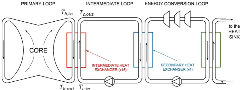
The conceptual scheme of the MSFR BoP is shown in
Figure 1. As it can be seen from thefigure, the non-nuclear part of the plant consists of a conventional circuit with two loops in series: (i) the Intermediate Loop, through which a fluoride-based molten salt circulates, serves to extract the heat generated in the reactorthrough an Intermediate Heat Exchanger (IHX) [10] and to transport it to the power conversion system; (ii) the Power Conversion Loop, which consists of a conventional Joule-Brayton gas-turbine cycle [11].
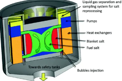
2.1 Reactor fuel circuit and core
The main conceptual feature that distinguish the MSFR is the nuclear fuel that is dissolved in a liquid fluoride- or chloride-based salt which acts contemporarily as fuel and coolant. The reference MSFR design [12] is a 3000 MWth
called‘sectors’) including the inlet and outlet pipes, a gas injection system, salt-bubble separators, pumps and fuel heat exchangers. Sixteen cooling sectors are arranged circumferentially around the vessel. Due to the liquid nature of the nuclear fuel, which does not require the presence of any solid fuel-element, and the fast neutron spectrum which does not require any moderating materials, the MSFR core is constituted by a simple, empty cavity, surrounded by an axial reflector and a radial blanket. The fuel salt, with an inlet temperature of about 650°C, enters radially from the bottom into the active zone, where it temporarily reaches criticality and its heated to the outlet temperature of about 750°C. The fuel then exits from the top of the core and it is recirculated through the 16 fuel sectors.
2.2 MSFR potentialities
Thanks to its peculiar features, the MSFR presents numerous advantages that make it attractive for the long-term perspective of the nuclear energy. It can operate with very flexible fuel-cycle strategies, reaching high breeding ratios with the thorium cycle, and it is capable
to operate as a waste-burner for transuranic waste produced in traditional once-through nuclear reactors, thereby allowing a significant reduction in radiotoxicity [13]. The liquid nature of the fuel allows adjusting on-line the fissile content, with the consequence that no excess reactivity is required in the core at any time to compensate for temperature and power defects, or to compensate fission-products-related reactivity losses. This means that neither burnable poisons nor long-term-adjustment control rods are needed in the core. The continuous removal of fission products allows a better chemical control and allows removing any FPs-related negative reactivity. In particu-lar, the removal of the main nuclear poison Xenon eliminates the reactor dead-time following shutdowns or power reductions, paving the way to much more flexible reactor operation and load-following applications. Great advantages are also present looking at the intrinsic safety aspects of the MSFR. Since the fuel is in afluid state, the core meltdown scenario is eliminated by-design and no limits exist for the attainable fuel burnup with respect to rods cladding damage andfission gas release. The low vapor tension of the molten salt allows operating the reactor at atmospheric pressure, reducing mechanical stresses on structural components and excluding all high-pressure-related accidental scenarios. Besides, in case of accidents an emergency fuel-draining system allows to automatically and passively drain the whole fuel content of the reactor, to assure its sub-criticality, and to passively cool it long-term [14]. Finally, the dual fuel/coolant role of the salt, together with its neutronics characteristics, implies that the MSFR has very large, negative, prompt temperature and void reactivity feedback coefficients, making the reactor extremely stable [15].
3 MSFR plant simulator modelling
In the perspective of identifying effective plant control strategies for an innovative reactor concept like the MSFR, an essential preliminary step was to acquire sufficiently accurate knowledge and understanding of both the reactor system dynamics and the whole Balance of Plant dynamics. To this aim, a control-oriented plant-dynamics simulator was developed and then used to study the MSFR dynamics. A proper dynamic simulation tool for control-oriented purposes, especially in a preliminary design phase, should satisfy some basic requirements [4,5]. In particular it should be
– modular and extensible, in order to be easily modified and updated to follow the design evolutions;
– readable, to allow an easy understanding of the equations implemented;
– computationally efficient, to allow fast-running and real-time simulations;
– be easily integrable with the control system model. With the above requirements to be fulfilled, the modelling choice fell on the Modelica language [3]. Modelica is an object-oriented, acausal, equation-based language which offers great advantages in terms of modularity, extensibility, readability and integrability with control-dedicated software (e.g. MATLAB control Fig. 2. MSFR fuel circuit conceptual scheme.
toolbox). The simulator was implemented within the Dymola simulation environment [7], which is equipped with state-of-the-art implicit numerical integration algorithms (e.g. DASSL) to handle non-linear differen-tial-algebraic equations sets and with effective homo-topy-based model-initialization algorithms [16], and which provides powerful model-linearization tools poten-tially useful in the future control system design phase. The tested and validated ThermoPower thermal-hydrau-lic Modethermal-hydrau-lica library [4] has been used for the simulator modelling, and it has been significantly modified and extended into an MSR library to account for all the balance equations pertaining the various nuclear varia-bles (see Sect. 3.1).
3.1 Fuel circuit and core
The usual approach employed for dynamics and control in conventional solid-fueled reactors is the so-called Point-Kinetics (i.e., zero-dimensional kinetics) [5,6]. In a circulating-fuel reactor like the MSFR the DNPs move along the fuel circuit, and a proper neutronics modelling needed to take into account the position of emission of the delayed neutrons in the core. Besides, a fraction of the delayed neutrons are emitted in the out-of-core portion of the primary circuit, thereby reducing the effective delayed neutron fractionbeff[17], with a clear impact on the reactor
dynamics. An ad-hoc neutronics model, which is able to take into account the DNPs position in the core, was therefore developed using a hybrid 0D-1D approach. Similar approaches have been proposed in previous works on circulating-fuel reactors’dynamics [18]. The conceptual scheme adopted for the fuel circuit modelling is shown in
Figure 4.
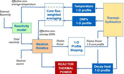
The circuit thermal-hydraulics determines the spatial distribution of the DNPs concentration along the fuel circuit. The DNPs spatial profile is then used to compute an effective core-averaged value of the DNPs concentra-tion in the core, suitable to be used in the reactor kinetics equation [19]. To correctly account for the drift of the DNPs, i.e., the fact that they are created in a different location with respect to the emission of the corresponding delayed neutron, in the averaging procedure the delayed neutron source intensity can be weighted with a neutron-importance function that can be both the direct flux or more properly the adjoint neutronflux [20]. Similarly, the average temperature used for the feedback reactivity evaluation is obtained as weighted-average of the temperature profile in the core multiplied by the importance function. The decay heat distribution was modelled using the same 1-D modelling approach. The total reactor power is the sum of thefission power in the core and the decay power throughout the whole fuel circuit.
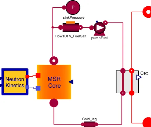
The Modelica model of the fuel circuit is shown in
Figure 5. The thermal-hydraulics of the reactor core was modelled in the MSR_Core component (Fig. 5). It is described by the mass (Eq.(1)), X-momentum (Eq.(2)), energy (Eq.(3)) conservation equation and the balance for the DNPs concentration for the 8 DNPs groups (Eq. (4)) and Decay Heat (DH) concentration for the 3 decay-heat groups (Eq. (5)). In the last three equations, the generation term due to thefission process is included. Longitudinal heat and species diffusion were neglected.
A∂d
∂tþ
∂w
∂x¼0 ð1Þ
∂w
∂xþA
∂p
∂xþAdg
∂z
∂xþ
Cfv
2dA2wjwj ¼0 ð2Þ
Ad∂h
∂tþw
∂h
∂x¼Aðq
000
fissþq000DHÞ ð3Þ
∂cg
∂t þ w Ad
∂cg
∂x ¼
bg
Lnfissclgcg g¼1;. . .;8 ð4Þ
∂Fk
∂t þ w Ad
∂Fk
∂x ¼fklDH;kq
000
fisslDH;kFk k¼1;2;3: ð5Þ
The RHS source termsq000fissandq000DHin equation(3)are the fission power density and the decay-heat generation density, respectively. The friction coefficientCfappearing
in the momentum equation (2) is evaluated using the Colebrook hydraulic correlation [21].
The termcis the neutron importance function and it was assumed to be fixed and equal to the fundamental eigenfunction of the single-energy diffusion theory for bare uniform reactori.e., a sinusoidal profile with a proper extrapolation length (Eq. (6)). The values of the fission heat concentrationq000fiss and decay heat concentrationq000DH
are computed from equations(7)and(8).
c¼cðxÞ ¼sin p x
Le
ð6Þ
q000fissðx;tÞ ¼ QfissðtÞ
AcoreRcdxcðxÞ ð7Þ
q000DHðx;tÞ ¼X
k
Fkðx;tÞ: ð8Þ
The time evolution of the normalized corefission power nfiss(t) =Qfiss(t)/Qfiss,0 is determined in the Neutron_
Kineticscomponent by the reactor-kinetics equation (9), in which the effective, neutron-importance-weighted averages of the DNPs concentrations equation (10)
are used, noting that, in the single-energy diffusion theory approximation, the neutron-importance function is taken as the neutronflux profile.
dnfiss
dt ¼
drtotb
L nfissþ X
g
lgcg;effþS ð9Þ
cg;effðtÞ ¼ R
cðxÞcgðx;tÞdx
R
cðxÞ
½ 2dx : ð10Þ
The total reactivityequation(11)is the sum of the externally inserted reactivity drext and the feedback
reactivity of fuel salt temperature and density. The latter two are determined by equations(12) and(13), where the effective temperature Teff is determined as a
neutron-importance-weighted core averageequation(14)and Teff,0is the reference temperature with respect to which the
reactivity defects are calculated. The effective delayed neutron fractions, which take into account the spatial distributions of the DNPs and the importance of the emitted neutrons, are evaluated according to equation(15).
drtotðtÞ ¼drextðtÞ þdrTðtÞ þdrdensðtÞ ð11Þ
drTðtÞ ¼aT½TeffðtÞ Teff;0 ð12Þ
drdensðtÞ ¼adens½TeffðtÞ Teff;0 ð13Þ
TeffðtÞ ¼
R
cðxÞTðx;tÞdx
R
cðxÞdx ð14Þ
beffðtÞ ¼
R
cðxÞlgcgðx;tÞdx
R
cðxÞ nfissðtÞ
L cðxÞ þ
X
g
lgcgðx;tÞ
( )
dx
: ð15Þ
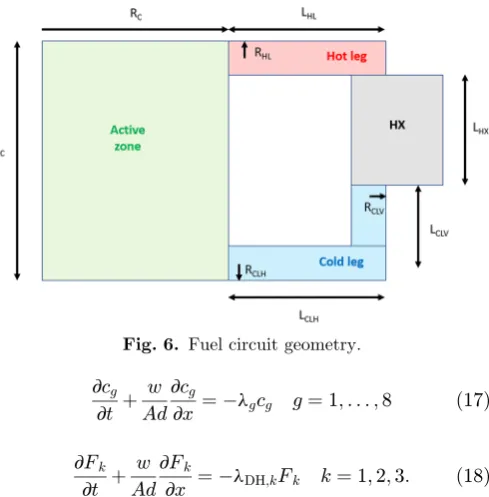
The 16 external loops forming the fuel circuit were modelled as a single equivalent loop formed by a hot leg section, representing the piping from the core outlet to the IHX inlet, the IHX and a cold leg section representing the piping from the IHX outlet to the core inlet (Fig. 6). The HotLeg and Cold leg tube components implement the single-state, one-dimensional, finite-volume-discretized conservation equations for mass (Eq.(1)) and momentum (Eq.(2)), whereas energy (Eq.(16)), DNPs (Eq.(17)), and DH (Eq.(18)) equations are modified to consider only the decay term.
Ad∂h
∂tþw
∂h
∂x¼vq
00
exchþAq000DH ð16Þ
MSR Core Neutron Kinetics P sinkPressure
Flow1DFV_FuelSalt pumpFuel
Qex
Cold_leg
∂cg
∂t þ w Ad
∂cg
∂x ¼ lgcg g¼1;. . .;8 ð17Þ
∂Fk
∂t þ w Ad
∂Fk
∂x ¼ lDH;kFk k¼1;2;3: ð18Þ
Ideal, mass-flow-rate-controlled pumps (PumpFuel component) establish the saltflow through the circuit.
The reactor total power is the sum of thefission power in the core and the decay heat generated along the whole fuel circuit equation (19). Reactor geometrical, opera-tional, physical and neutronic data used in the following are shown inTables 1and2(with reference toFig. 6). All the parameters of the simulator are easily modifiable at runtime to allow for model modification and update throughout the various design phases.
Qreactorð Þ ¼t Qfissð Þ þt
Z
fuel circuit
Aq000DHðx;tÞdx: ð19Þ
Since the fuel circuit forms a closed loop, it was important to provide an expansion tank to avoid strong pressure variations caused by temperature transients. The SinkPressurecomponent allows handling any mass insurge or outsurge transient, with no associated dynamic effect. When massflows from the sink to the loop, the outsurge fluid was assumed to be at the same temperature of the cold leg.
3.2 Intermediate heat-exchanger (IHX)
Due to its non-conventional design, an effort was spent to set up a specific component representing the MSFR intermediate heat exchangers [10]. The heat exchangers were modelled as counterflow heat exchangers, with particular reference to the Printed Circuit Heat Exchanger
a proposed technology for the MSFR, for more detail see [11] but any other counterflow arrangement based on parallel flow pipes subject to heat transfer through their lateral surface can be modelled as well with little modification. The Intermediate_HX model (Fig. 5) is based on components from the ThermoPower library,
especially theFlow1DFVcomponent, which describes the fluidflow in a rigid tube. It is based on a 1Dfinite volume discretization of the mass (Eq.(20)), momentum (Eq.(21)) and energy transport (Eq.(22)) equations:
A∂d
∂tþ
∂w
∂x¼0 ð20Þ
∂w
∂t þA
∂p
∂xþAdg
∂z
∂xþ
Cfv
2dA2wjwj ¼0 ð21Þ
Ad∂h
∂tþw
∂h
∂x¼vq
00
exch: ð22Þ
The geometrical parameters that can be specified in the component are the lengthL, the cross-section areaAand the heat transfer perimeter v, which for a PCHE are expressed as
A¼pd
2 ch
8 ð23Þ
v¼dch 1þp
2
ð24Þ
where dch is the channel diameter. Figure 7 shows the
Modelica model of the IHX whereas the geometric and operational parameters are shown in Table 3. One-dimensional finite-volume discretization with counter-current flows was employed for the heat transfer in the heat exchanger. A single, equivalent heat exchanger component, representative of the 16 parallel ones (one for each of the parallel fuel circuit loops), was used. Longitudinal heat transfer along the flow direction was neglected, while the heat capacity of the metal walls of the heat exchanger was accounted for. Equations(25)and(26)
are the heat exchange equations on the hot (fuel salt) and cold (intermediate salt) sides, respectively. Equation(27)
is the energy balance equation for the IHX metal wall.
q00hot¼hhotðTfuel saltTw;hotÞ ¼
k
s=2ðTw;hotTvolÞ ð25Þ
q00cold¼hcold Tint saltTw;cold
¼ k
s=2 Tw;coldTvol
ð26Þ
vq00hotþq00cold¼Amdmcm
dTvol
dt : ð27Þ
Due to the small channel size, the resultingflow is laminar in most of the cases for the fuel salt side. This simplifies considerably the heat transfer modelling (even if it restricts the heat transfer coefficients to quite low values). The average Fanning friction factor (Eq. (28)) and Nusselt number (Eq.(29)) for fully developed laminarflow in semi-circular ducts [22] were implemented. In equations, it reads:
f ¼15:767
Re ð28Þ
Nu¼4:089: ð29Þ
On the cold (intermediate salt) side theflow regime is in the transition zone (Re≈50007000), and the Gnielinski [21] correlation (Eq.(30)) is used.fDarcy(Re) is the Darcy
friction factor, for which the Petukhov [21] correlation for smooth tubes (Eq.(31)) is used
Nu¼
fDarcy=8
Re1000
ð ÞPr
1þ12:7 fDarcy=8
1=2
Pr2=31
ð30Þ
fDarcy¼ ð0:79 lnðReÞ 1:64Þ2: ð31Þ
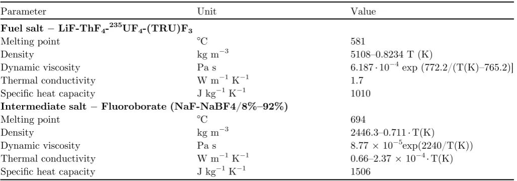
Table 1. Physical properties of fuel and intermediate salt [23,24].
Parameter Unit Value
Fuel saltLiF-ThF4-235UF4-(TRU)F3
Melting point °C 581
Density kg m3 5108–0.8234 T (K)
Dynamic viscosity Pa s 6.187·104exp (772.2/(T(K)–765.2)]
Thermal conductivity W m1K1 1.7
Specific heat capacity J kg1K1 1010
Intermediate saltFluoroborate (NaF-NaBF4/8%–92%)
Melting point °C 694
Density kg m3 2446.3–0.711·T(K)
Dynamic viscosity Pa s 8.77105exp(2240/T(K))
Thermal conductivity W m1K1 0.66–2.37104·T(K)
Specific heat capacity J kg1K1 1506
Table 2. MSFR geometric, operational and physical parameters.
Parameter Symbol Value Parameter Symbol Value
Geometric and operational parameters
Core length LC 1.9 m Reactor thermal power Qreactor 3000 MWth
Core radius RC 1.23 m Fuel massflow rate – 29703 kg s1
Hot leg length LHL 0.65 m Intermediate massflow rate – 28458 kg s1
Hot leg radius RHL 0.15 m Number of sectors – 16
IHX length LHX 0.52 m Core inlet temperature Tcore_in 675°C
Cold leg lengthvertical LCLV 1.38 m Core outlet temperature Tcore_out 775°C
Cold leg radiusvertical RCLV 0.15 m Intermediate salt IHX inlet temp. Tint_min 670°C
Cold leg lengthhorizontal LCLH 0.65 m Intermediate salt IHX outlet temp. Tint_max 600°C
Cold leg radiushorizontal RCLH 0.15 m Extrapolation Length 0.10 m Neutronic parameters
DNP fractiongroup 1 b1 12.3105 DNP decay constant group 1 l1 0.0125 s1
DNP fractiongroup 2 b2 71.4105 DNP decay constant group 2 l2 0.0283 s1
DNP fractiongroup 3 b3 36.010 5
DNP decay constant group 3 l3 0.0425 s 1
DNP fractiongroup 4 b4 79.4105 DNP decay constant group 4 l4 0.133 s1
DNP fractiongroup 5 b5 147.410 5
DNP decay constant group 5 l5 0.292 s 1
DNP fractiongroup 6 b6 51.5105 DNP decay constant group 6 l6 0.666 s1
DNP fractiongroup 7 b7 46.6105 DNP decay constant group 7 l7 1.63 s1
DNP fractiongroup 8 b8 15.1105 DNP decay constant group 8 l8 3.55 s1
DNP fractiontotal b 459.7105 Neutron generation time L 6.65 × 10⁷s Doppler feedback coefficient aT –1.46 pcm K
1
Density feedback coefficient adens –2.91 pcm K 1
Decay heat parameters
DH fractiongroup 1 f1 0.0117 DH decay constantgroup 1 lDH,1 0.01973 s1
DH fractiongroup 2 f2 0.0129 DH decay constantgroup 2 lDH,2 0.0168 s1
The thermohydraulic correlations to be used in the IHX component are selectable at runtime, to allow for design variations in geometrical and/or operational IHX parameters.
3.3 Intermediate loop and secondary heat-exchanger (SHX)
The four intermediate loops were modelled as a single equivalent loop formed by a hot leg section, representing the piping from the IHX outlet to the SHX inlet, a bypass line and a cold leg section representing the piping from the SHX outlet to the IHX inlet (Fig. 8). The intermediate loop model was assembled by using standard components from the ThermoPower library. The adopted scheme is represented inFigure 8. The two basic components are the hotLeg and coldLeg compo-nents, which are modelled by Flow1DFV objects. The transport delay associated with the hot/cold leg, with the geometrical parameters indicated in Table 4, is of the order of some seconds. In addition, the dynamic effect associated with thermal inertia is not negligible, hence the total volume of the intermediate loop has a significant influence on dynamics.
The loop includes two active components, a pump and a bypass valve (Fig. 8). The pump class models a simple centrifugal pump with no energy or momentum dynamics and the power consumption was simply estimated through a constant pump efficiencyhp. The pump has an external
input port which can be used to control the rotational speed and thus the mass flow rate. The valve component was modelled by theValveLinclass, which simply provides a linear constitutive equation to relate the pressure dropDpv
and the bypass massflow rateGbypass:
Gbypass¼KvcmdDpv ð32Þ
whereKvis a hydraulic conductance parameter set to 102
and cmd is the command signal, provided by an external input port. The valve can be used to control the massflow rate flowing in the secondary heat exchanger, providing another way to control heat extracted from the intermedi-ate loop. As explained inSection 3.1for the fuel circuit, an expansion tank was provided to avoid the strong pressure variations related to temperature transients of an incom-pressible liquid in closed loop and to establish a reference pressure level in the cold leg (1 bar). The expansion tank was modelled using theexpansionTankcomponent (Fig. 8). The other components appearing in Figure 8 are simple temperature and massflow rate sensors, which model zero-order sensors providing ideal measurements. Geometric and operational parameters of the intermediate loop are shown inTable 4.
In the SHX, heat is transferred from the intermediate salt to the helium in the Energy Conversion System (ECS). The modelling approach employed for the SHX was identical to that used for the IHX (see Sect. 3.2). Geometric and operational parameters are shown in
Table 4. Theflow regime in the SHX is fully turbulent on both the salt and gas sides (ReD≈4104 and ReD≈
1.5105, respectively). The Gnielinski [21] correlation is used to evaluate the convective heat transfer coefficients. Also in this case, the correlations to be used in the SHX component are selectable at runtime, to allow for design variations in geometrical and/or operational SHX parameters.
Q_ex
Fig. 7. Object-oriented Modelica model of the IHX.
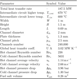
Table 3. Geometric and operational parameters of the IHX.
Parameter Symbol Value
Total heat transfer rate – 187.5 MW Intermediate circuit higher temp. Tc,out 670°C
Intermediate circuit lower temp. Tc,in 600°C
Width W 1 m
Height H 1.5 m
Length L 0.69 m
Channel diameter dch 2 mm
Plate thickness tp 1.3 mm
Channel pitch pch 2.5 mm
Channels number nch 240,000
Global heat transfer coeff. U A 3.02 MW K1 Hot channel Reynolds number Reh 238
Cold channel Reynolds number Rec 5631
Hot channel average velocity uh 1.14 m s1
Cold channel average velocity uc 2.66 m s1
Hot channel pressure drop Dph 3.96 bar
Cold channel pressure drop Dpc 1.30 bar
3.4 Energy conversion system (ECS)
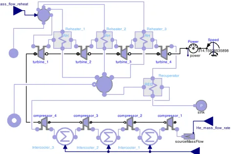
The energy conversion system model was assembled by using standard components from the ThermoPower library. In particular, a Helium Joule-Brayton cycle with regeneration and three stages of reheating and intercooling was considered. This configuration turned out to ensure a gas temperature at secondary heat exchanger inlet that can avoid salt solidification problem [11]. The adopted scheme is represented in
Figure 9.
There are five main components in the model, namely, the compressor, the turbine, the intercooler, thereheater, and therecuperator(Fig. 9). The cycle was modelled as open, i.e., disregarding the final heat sink section. This is a common choice to simplify the modelling of the cycle [5] and it has no impact on the dynamics results since the final sink acts as an infinite heat sink.
3.4.1 Compressor
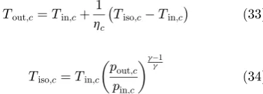
The compressor was modelled by considering an energy balance. Since Helium can be considered as perfect gas, the following relations hold:
Tout;c¼Tin;cþ 1
hc
Tiso;cTin;c
ð33Þ
Tiso;c¼Tin;c
pout;c
pin;c
g1
g
ð34Þ
whereTin,candpin,care the gas temperature and pressure
at the inlet of the compressor,Tout,candpout,care the gas
temperature and pressure at the outlet of the compressor, hcis the compressor efficiency,Tiso,cis the isentropic outlet
set by the user in order to adapt the component to the cycle parameters. The component can be connected to a shaft in order to calculate the compressor work (and hence the cycle efficiency).
3.4.2 Turbine
The turbine was modelled by considering an energy balance similar to that used in compressor component. In particular,
Tout;t¼Tin;thtðTin;tTiso;tÞ ð35Þ
Tiso;t¼Tin;t
pout;t
pin;t
g1
g
ð36Þ
whereTin,tandpin,tare the gas temperature and pressure
at the inlet of the turbine, Tout,t and pout,t are the gas
temperature and pressure at the outlet of the turbine, ht
is the turbine efficiency, Tiso,t is the isentropic outlet
temperature of the turbine. Also, in this case, the efficiency and the pressure ratio are user-selectable parameters and the turbine work can be calculated.
Table 4. Geometric and operational parameters of the SHX.
Parameter Value
Intermediate loop
Hot leg length 5 m
Hot leg radius 0.75 m
Cold leg lengthhorizontal 5 m
Cold leg radiushorizontal 0.75 m
Cold leg lengthvertical 0.82 m
Cold leg radiusvertical 0.75 m
Secondary heat exchanger
Total heat transfer rate 750 MW
Intermediate circuit higher temp. 670 °C Intermediate circuit lower temp. 600 °C
Inlet gas temperature 460 °C
Outlet gas temperature 615 °C
Length 1.51 m
Channel diameter 10 mm
Plate thickness 6 mm
Channels number 250,000
P
sink
Power
power
Speed
turbine_1
sourceMassFlow
compressor_1 compressor_2
compressor_3
turbine_2 turbine_3
compressor_4
turbine_4
Reheater_1
RH RH
Reheater_2
RH RH
Reheater_3
RH RH
Intercooler_1 Intercooler_2
Intercooler_3
REG
Recuperator
He_mass_flow_rate
T_intercooling mass_flow_reheat
314.15926535898
3.4.3 Intercooler
The intercooler is a heat exchanger with the gas and an infinite sink at prescribed temperature (T_intercooling). It is adopted to improve efficiency by decreasing the average specific volume of the gas in the compression stages.
3.4.4 Reheater
The reheater is a heat exchanger with the gas at the outlet turbine and a hotter source. It is adopted to improve efficiency by increasing the average specific volume of the gas in the expansion stages. In the present model, a fraction of the gas at the secondary heat exchanger outlet is extracted to reheat the colder gas at the turbine outlet. An alternative option is to employ the hot intermediate molten salt in the reheaters.
3.4.5 Recuperator
The recuperator is a heat exchanger aimed at performing regeneration, i.e., preheating the gas at the inlet of the secondary heat exchanger with the high temperature gas at the turbine outlet. This improves the efficiency and can also avoid the problem of the salt solidification in the secondary heat exchanger.
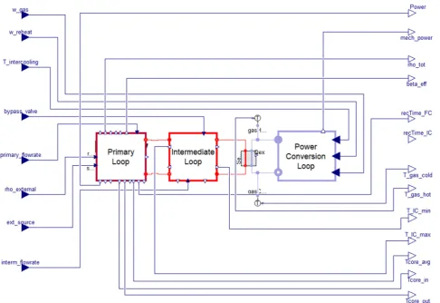
3.5 Full plant simulator
The MSFR plant simulator model was built assembling the various sub-models illustrated inSections 3.1through3.4. The full, coupled, Modelica model is shown in Figure 10, whileTable 5 shows the various model input and output variables. Table 6 summarizes various meaningful plant variables in steady-state nominal operating conditions, as obtained with the present plant simulator.
4 Analytical benchmark model
An analytical model was developed to verify the DNPs model implemented in the MSFR power plant simulator and the corresponding values of the effective delayed neutron fractionsbeff,gfor the various delayed groups. The
The presence of a reflector was allowed for through the introduction of a proper extrapolation length.
f∝J0 2:405 r
Re
cos p z
He
: ð37Þ
The fuel salt velocity profile was assumed fixed and axially directed, the motion occurs in the form of parallel streamlines and DNPs turbulence mixing and molecular diffusion were neglected. Two different velocity profiles were considered, a uniform one and a parabolic one. The out-of-core portion of the circuit was modelled with a 0-D geometry, i.e., with a simple, mass-flow-rate-dependent, out-of-core timetout. It was assumed that, in the
out-of-core portion of the fuel circuit, complete fluid mixing occurs. The DNPs re-entry boundary condition at core inlet was therefore assumed to be uniform, and equal to the
average outlet concentration, reduced by the fraction of DNP which decays in out-of-core portion of the circuit. All physical properties were considered constant and evaluat-ed at the core average temperature. Geometric, operational and physical parameters used in the following are shown in
Table 7.
Under the above modelling assumptions, the DNPs balance equation is:
u rð Þ∂Cgðr;zÞ
∂z ¼bg n0
LJ0 2:405
r Re
cos p z
He
lgCgðr;zÞ
ð38Þ
where
n0¼Z P0Ln=wf
þH=2
H=2 Z R
0
J0 2:405 r Re
cos pHz
e
2prdrdz
n o ð39Þ
Table 5. Description of the simulator input and output variables.
Input Description
Primary Loop
rho_external External reactivity source
primary_flowrate Fuel circuit massflow rate (all 16 sectors)
ext_source External neutron source
Intermediate Loop
interm_flowrate Intermediate circuit mass flow rate (all 4 loops)
bypass_valve Bypass circuit valve opening
Power Conversion Loop
w_gas Turbine gas massflow rate
w_reheat Reheating gas massflow rate
T_intercooling Temperature of gas cooling and intercooling
Output Description
Primary Loop
Power Reactor thermal power
rho_tot Total reactivity variation (relative to starting steady-state)
beta_eff Total effective delayed fraction for circulating fuel
recTime_FC Fuel circuit salt recirculation time
Tcore_avg Effective core-average temperature
Tcore_in Core inlet salt temperature
Tcore_out Core outlet salt temperature
Q_intHX (not shown) Intermediate HXs total heat transfer rate
rho_T (not shown) Reactivity variation due to temperature feedback
rho_dens (not shown) Reactivity variation due to density feedback Intermediate Loop
T_IC_min Max temperature of intermediate salt (IHX outlet)
T_IC_max Min intermediate salt temperature (SHX outlet)
recTime_IC Intermediate loop salt recirculation time
Q_secHX (not shown) Secondary HXs total heat transfer rate (all 4 units) Power conversion loop
mech_power Turbine mechanical power
T_gas_hot Gas temperature at SHX outlet
uðrÞ ¼uzðrÞ ¼
G
rAcoreyðrÞ ð40Þ
where with y(r) is indicated the velocity profile shape, which for uniform velocity is y(r) = 1 and for parabolic velocity is y(r) = 2(1r2/R2). Under the hypothesis of parallel streamline flow, equation (38) can be solved analytically, resulting in equation (41) for the DNPs concentrations. The core inlet boundary condition Cg,in
under the complete mixing assumption is expressed by equation (42). Having obtained the DNPs spatial distri-butions, the effective delayed neutron fractions beff,g are
calculated taking into account the spatial neutron-impor-tance of the emitted neutrons, according to equation(43)
[17], approximated with the direct neutronflux.
See equations(41)–(43)below.
Figure 11 shows the comparison between the trend
against the fuel salt mass flow rate of the steady-state effective delayed fractionsbeff,gas predicted by the Dymola
1-D plant simulator and those predicted by the analytical MATLAB 2-D model for the two velocity profiles.Figure 11
also shows the values of the delayed fractions for static fuel beff,statand those predicted by a lumped-parameter model
[25] according to the expression:
bg;lump¼
bg
1þ1elgtout
lgtcore
: ð44Þ
Cgðr;zÞ ¼Cg;inðrÞe
lgtcore
yðrÞ ð12þHzÞ þb
g
n0
LJ0 2:405
r Re
tcore
yðrÞ
pH
He
2
þ lgtcore yðrÞ
2 lgtcore
yðrÞ cos p
z He
þpH
Hesin
p z
He
e
lgtcore
yðrÞ ð12þHzÞ lgtcore
yðrÞ cos
p 2 H He pH
Hesin p 2 H He ð41Þ
Cg;inðrÞ ¼Cg;in
¼ bg n0 L Z R 0
J0 2:405 r Re
tcore
yðrÞ
pHeH 2
þ lgtcore
yðrÞ
2
lgtcore yðrÞ cos
p
2 H He
1e
lgtcore
yðrÞ
þpH Hesin
p
2 H He
1þe
lgtcore
yðrÞ
8 > < > : 9 > = >
;yðrÞ2prdr
Acoreelgtout
Z R
0
e
lgtcore
yðrÞ
yðrÞ2prdr
ð42Þ
bg;eff¼
Z R
0 Z H=2
H=2
fðr;zÞlgCgðr;zÞ2prdrdz
X8 g¼1
Z R
0 Z H=2
H=2
fðr;zÞlgCgðr;zÞ2prdrdzþ Z R
0 Z H=2
H=2
fðr;zÞn0
LJ0 2:405Rre
cos pHz
e
2prdrdz
ð43Þ Table 7. Geometric and operational parameters used in the analytical 2-D MATLAB model.
Parameter Symbol Value Parameter Symbol Value
Core height H 1.90 m Reactor thermal power P0 3000 MWth
Core radius R 1.23 m Fuel mass flow rate G 29703 kg s1
Extrapolation length dex 0.10 m Salt average density r 4287 kg m3
Core transit time tcore 1.303 s Volumetricflow rate Q 6.929 m3s1
Out of core transit time tout 0.891 s Core average velocity um 1.4578 m s1
DNP fractiongroup 1 b1 21.8105 DNP decay constantgroup 1 l1 0.0125 s1
DNP fractiongroup 2 b2 47.6105 DNP decay constantgroup 2 l2 0.0283 s1
DNP fractiongroup 3 b3 39.3105 DNP decay constantgroup 3 l3 0.0425 s1
DNP fractiongroup 4 b4 63.5105 DNP decay constantgroup 4 l4 0.133 s1
DNP fractiongroup 5 b5 103.5105 DNP decay constantgroup 5 l5 0.292 s1
DNP fractiongroup 6 b6 18.1105 DNP decay constantgroup 6 l6 0.666 s1
DNP fractiongroup 7 b7 22.8105 DNP decay constantgroup 7 l7 1.63 s1
DNP fractiongroup 8 b8 5.210 5
DNP decay constantgroup 8 l8 3.55 s 1
Results shown in the following refers to parameters values indicated in Table 7. Note that, for reasons of comparison with previous works [26], the values of the static-fuel delayed fractions used in this section for purposes of verification of the DNPs model are slightly different from those employed for plant free dynamics simulation (Tab. 2). As can be seen fromFigure 11, the MSFR plant simulator predicts with sufficient accuracy the trend of the effective delayed fractions as a function of the fuel salt mass flow rate, when compared to the analytical 2-D model, in particular for the uniform velocity profile (for the parabolic velocity profile, the MATLAB model underestimates the effective delayed fractions in most of the massflow rate range: the reason is the higher fuel salt velocity near the core axis, which leads to lower DNP concentrations in a region of high neutron importance which are not compensated by the higher concentrations in the annular region due to the lower neutron importance of this zone). A small offset of about 10% is present for the saturation valuesi.e., the limiting values of thebeff,g for high flow velocity, when
the fuel circuit recirculation time is far less than the DNPs time constantstrecirc≪l1g due to the different modelling dimensionalities [18]. For small mass flow rates, the effective delayed fractions tend to their corresponding static-fuel values as can be seen for delayed groups 6 to 8 (the “fastest” groups). For the slowest groups (1 to 4), the static-fuel values are only reached at very low massflow rates, out of the simulated range of Figure 11. For these groups, in the simulated mass flow rate range the effective delayed fractions are essentially constant and equal to the corresponding saturation values. Figure 12 shows the dependency on the fuel massflow rate of the total delayed fractionbeff,tot
as predicted by the different models. An important fact that can be deduced from thefigures is that, in nominal conditions (G≈30 t/s,trecirc≈4 s),beff,totis almost
insensi-tive to small massflow rate variations, due to the fact that groups 1 through 5 are essentially at saturation. Since a variation ofbeff,totis equivalent to a reactivity insertion, this
fact has an impact on reactor dynamic behavior during transients (seeSect. 5.1).
5 Plant free dynamics simulation
The study of the plant free dynamics is a fundamental step in order to understand the behavior of a reactor in response to different transient initiators. It also provides the necessary insights on the plant to support the definition of suitable control strategies and operating procedures. In this section, the simulation results for four different transients are presented and analyzed: (i) fuel salt massflow rate reduction, (ii) intermediate salt mass flow rate reduction, (iii) turbine helium mass flow rate increase, and (iv) external reactivity insertion. All the transients were simulated starting from nominal full-power steady-state operating conditions. The plant simulator developed in the present work allows simulating transients of 200 s with computational times of less than 15 s (2.80 GHz with 16 GB memory laptop).
5.1 Reduction of the fuel salt massflow rate
(Fig. 13f), and the intermediate salt outlet temperature start to decrease (Fig. 13h). The reduced intermediate salt temperature then causes a corresponding decrease in the temperature of the helium at the turbine admission (Fig. 13m), which leads to a reduction of the turbine mechanical power output (Fig. 13i). When the transient initiator ends, the tradeoff between the increased fuel heating in the core and the increased fuel cooling in the IHX leads to a new equilibrium with a largerDT. At the end of the transient, the new average core temperature will be such that it exactly compensates the variation in the effective delayed neutron precursor fractionbeffdue to the
reduction of the fuels salt velocity. Thefinal value ofdrtotof
about4 pcm (Fig. 13b) therefore correspond toDbeff.
This transient feature is peculiar to circulating fuel reactors and of the MSFR in particular [25]. From any starting condition, a primary circuitflow velocity reduction causes an increase in the effective delayed neutron fraction b
eff, because less delayed neutrons precursors decayed outside in the core, and the delayed neutron are created in core positions of higher neutron importance (Sect. 4, [17]). This corresponds to a positive reactivity insertiondr=Dbeff. For
a zero-power reactor, i.e. neglecting feedback effects of temperature and density on the reactivity, this dr>0 causes reactor power to start increasing according to the inhour equation. If temperature feedback effects are included in the analysis, core temperature variations cause reactivity insertions, and, depending on the relative magnitudes of the negative “temperature-reactivity” and the positive“precursor-reactivity”, the reactor power might either decrease or increase. The exact features of the power evolution during the transient will depend on the starting power level (which determines the magnitudes of the temperature variations), the starting massflow rate (which determines thebeffdependency on the massflow ratesee Sect. 4), and on the operating parameters of the heat exchangers and of the energy conversion system. Starting from nominal full-power operating condition, it is clear fromFigure 13that a variation of the fuel massflow rate has an almost negligible impact on the reactor power level, with power variation below 1% at the end of the transient (Fig. 13a). The small differences (a few MWs, seeFigs. 13a and13f) between the reactor thermal power and the heat transfer rates in the two heat exchangers are due to the pumping powers in the fuel and intermediate circuits. It is instead evident the strong impact it has on the minimum and maximum temperatures of the fuel salt, with variations of about 12°C in opposite directions (Figs. 13c and13d).
5.2 Reduction of the intermediate salt massflow rate
A 20% intermediate mass flow rate reduction is considered. An exponential flow reduction with a time constant of 5 s was chosen to take into account the pumps’inertia. Simulation results are shown inFigure 14. As soon as the flow reduction begins, the reduced flow rate causes an increase of the intermediate salt maximum temperature, at the IHX outlet (Fig. 14h), and a decrease of the minimum temperature, at the outlet of the SHX (Fig. 14g), due to the increased residence time in the two heat exchangers. The reduced heat transfer rates
(Fig. 14f), due to the reduced velocity, cause core inlet temperature to increase (less power is removed,Fig. 14c), and gas temperature to decrease (less power is ceded,
Fig. 14m). When the hotter fuel salt startsfilling the core (Fig. 14e), the negative reactivity it provides (Fig. 14b) starts reducing the core power (Fig. 14a). Core inlet temperature reaches a maximum of about +5°C, and then decreases when the cooler intermediate salt reaches the IHX after its transit time. This maximum corresponds to the max negative reactivity value, and in turn to the lowest reactor power, at aboutt= 18 s. Due to this power minimum, the core outlet temperature reaches in turn a minimum at aboutt= 25 s. After all temperatures have reached corre-sponding local maxima/minima att= 18–25 s, the system slowly stabilizes to itsfinal new equilibrium state when the power extracted from the SHX matches the reduced reactor power (plus the pumping powers). The mechanical power of the turbine unit correspondingly decreases due to the reduction of the helium admission temperature. Intermediate flow rate has a small impact on reactor power and fuel salt temperatures, while it strongly influences the temperatures of the intermediate salt, especially its minimum value (Figs. 14g and14h).
5.3 Increase of the helium turbine massflow rate
5.4 External reactivity insertion
The fourth and last simulated transient consists of a 0.1 $ external reactivity step insertion. Simulation results are shown inFigure 16. As can be seen from Figure 16a, the reactor thermal power undergoes a prompt jump of about 20%. The average fuel temperature immediately increases of about 6°C in fractions of a second (Fig. 16e) due to the higherfission power, leading to a fast injection of negative reactivity thanks to the large negative prompt feedback coefficient (−1.46 pcm/K from Doppler feed-back,−2.91 pcm/K from density feedback) and the power rapidly decreases from the peak prompt-jump value. When the heated fuel salt (Fig. 16d) reaches the IHX, the heat transfer rate in the IHX increases (Fig. 16f) due to the higherDT, and the intermediate salt maximum tempera-ture starts increasing as a consequence. Similarly, when the hotter intermediate salt enters the SHX at about t= 9 s, the power extracted from the SHX increases and the helium temperature at turbine admission increases in turn. For a constant reheating gas mass flow rate (see
Sect. 3.4), the average helium temperature in the SHX also increases. When the hot fuel salt produced in the power peak re-enters the core, the average fuel tempera-ture has a slight increase that causes a second, sudden power decrease.
All the plant relevant temperatures are“dragged up”by the augmented fuel temperature. The system simply stabilizes at a higher temperature level, determined by the effective core temperature at which the feedback effects exactly compensate the external reactivity. In particular, for a 0.1 $ external reactivity insertion and a total feedback coefficient of 4.37 pcm/K, this corresponds to about 11.5°C temperature increase in the core, other temper-atures being determined by heat transfer in the HXs. Since all the temperatures shift upward following the fuel temperature, the final post-transient value of the latter can be reached at a reactor power level that is very similar to the starting value: a 0.1 $ insertion causes a variation of less than 2% in the reactor thermal power (Fig. 16a) and of about 3% in the turbine mechanical power (Fig. 16i) (the discrepancy is due to the varying thermodynamic efficiency of the cycle at varying temperatures). The practical consequence is that external reactivity is not a suitable input variable for power regulation. On the other hand, it has a strong impact on all plant temperatures.
5.5 Outcomes of the MSFR dynamic simulations
From the results of the simulated transients, valuable insights in the reactor behavior, useful for the definition of the normal operating procedures and the selection of reactor control strategies, can be obtained:
–The plant dynamics analysis for a reactivity insertion transient clearly shows that an insertion of external reactivity has a small effect on the reactor power. In this perspective, an external reactivity system is not required for the load-following capabilities in terms of power variation.
–The MSFR shows a typical reactor-follows-turbine behavior in which is the ultimate heat loop extraction (i.e., the energy conversion system) that drives the core
power. This confirms the need to include the modelling of this loop in a power plant simulator aimed at studying the control strategies. In this view, the most suitable candidate for controlling the reactor power output seems to be the helium massflow rate.
– The fuel massflow rate has small effect on the power. This comes from the design choice of using the printed circuit heat exchangers for the intermediate HX. In particular, the laminar condition imposed by this type of HX does not allow strong variation in the heat transfer properties when changing the fuel velocity. The fuel mass flow rate variation has a remarkable impact on the inlet and outlet core fuel temperature.
– Settling times to post-transient equilibrium values are of the order of 100–150 s for all the considered transients. The dynamics of the plant is mainly governed by the heat capacity in the HXs rather than physical recirculation time. The characteristics time of the MSFR is strongly influenced by the choice of the metal HX material and its configuration, and different design options for the heat exchangers will lead to different dynamics feature of the reactor.
6 Conclusions
In this paper, a plant-dynamics simulator oriented to the control design of the MSFR power plant was developed by employing the well tested,flexible and open-source object-oriented Modelica language. Components from validated thermal-hydraulic libraries were used to model the intermediate circuit, the energy conversion system and the heat exchangers, and a new library was created to model the 1-D flow of a liquid nuclear fuel, with the associatedfinite-volume-discretized balance equations for the DNPs concentration and the decay heat density. In particular, an effort was spent in implementing an ad-hoc hybrid 0D-1D neutron-kinetics which properly takes into account the position of the DNPs along the fuel circuit and the consequent reactivity insertion due to the variation of the effective delayed fractions. In addition, an analytical steady-state 2-D model of the core and the fuel circuit was developed using MATLAB in order to verify the DNPs model.
The simulator was then employed to investigate the MSFR power plant free dynamics in response to four typical design-basis transient initiators. Computational times for all the considered transients are of the order of a few seconds, proving the simulator to be a very computationally-efficient tool.
Starting from the insights on the reactor behavior gained from the analysis of its free dynamics here presented, and thanks to the characteristics of the Modelica language in terms offlexibility and integrability with control design software (e.g. MATLAB Control System Toolbox), the plant simulator here developed will provide a valuable tool in support to thefinalization of the design phase and to the definition of model-based plant control strategies.
This project has received funding from the EURATOM research and training programme 2014-2018 under grant agreement No 661891.
Author contribution statement
C. Tripodo developed the core and fuel circuit models, and implemented the power plant simulator. A. Di Ronco developed the intermediate loop and power conversion loop models. C. Tripodo and S. Lorenzi carried out the numerical simulations, and analyzed and interpreted the results. C. Tripodo wrote the manuscript with input and feedback from S. Lorenzi. A. Cammi and S. Lorenzi conceived the presented idea, supervised the work and offered assistance throughout the project.
Disclaimer
The content of this paper does not reflect the official opinion of the European Union. Responsibility for the information and/or views expressed therein lies entirely with the authors.
Nomenclature
Acronyms
ALFRED Advanced Lead Fast Reactor European Demonstrator
BoP Balance of Plant
DNP Delayed Neutron Precursor
FP Fission Product
GIF-IV Generation-IV International Forum IHX Intermediate Heat Exchanger MSFR Molten Salt Fast Reactor PCHE Printed Circuit Heat Exchanger
SAMOFAR Safety Assessment of the Molten Salt Fast Reactor
SHX Secondary Heat Exchanger
Latin symbols
A Cross sectional area (m2) Cf Friction coefficient ()
cg Normalized precursor density forgth group ()
Cg Precursor density forgth group (m3)
cmd Bypass valve command signal () d Density (kg m3)
dch Channel diameter of heat exchanger (m)
Dhyd Hydraulic equivalent diameter (m)
f Fanning friction factor () fDarcy Darcy friction factor ()
fk Decay heat fraction forkth group ()
Fk Decay heat density forkth group (W m3)
g Gravitational acceleration (m s2) Gbypass Bypass massflow rate (kg s1)
h Specific enthalpy (J kg1)
hcold Cold side convective heat transfer coefficient
(W m2K1)
hhot Hot side convective heat transfer coefficient
(W m2K1) H Core height (m)
He Core extrapolated height (m)
J0 Zero order Bessel function ()
k Thermal conductivity (W m1K1)
Kv Hydraulic conductance parameter (kg s1Pa1)
Le Core extrapolated length (m)
n0 Neutron density at core center (m3)
nfiss Normalizedfission power ()
Nu Nusselt number () p Pressure (Pa)
P0 Nominal reactor power (W)
Pr Prandtl number () q00 Heatflux (W m2) q000 Power density (W m3)
Q Power (W)
r Radial coordinate (m) R Core radius (m)
Re Core extrapolated radius (m)
Re Reynolds number () s HX wall thiness (m)
S External neutron source (s1)
t Time (s)
T Temperature (K) u Axial velocity (m s1) w Massflow rate (kg s1)
wf Averagefission energy (Jfiss1)
x Coordinate along fuelflow (m) z Vertical coordinate (m)
Greek symbols
a Reactivity feedback coefficient (K1) b Delayed neutron fraction () g Specific heat ratio ()
G Fuel mass flow rate (kg s1) h Isentropic efficiency ()
_
u Angular velocity (rad s1)
lDH,k Decay heat decay constant forkth group (s1)
lg DNP decay constant forgth group (s1) L Effective neutron lifetime (s)
n Emitted neutron perfission (fiss1) f Neutronflux 2-D profile shape () dr Reactivity variation ()
tcore Core transit time (s)
tout Out-of-core transit time (s)
trecirc Fuel circuit recirculation time (s)
Subscripts
0 Starting steady-state value c Compressor
cold Cold side dens Density DH Decay Heat eff Effective exch Exchange ext External fiss Fission
g DNP group
hot Hot side in Inlet
int Intermediate k Decay heat group lump Lumped
m Metal
out Outlet
t Turbine
tot Total vol Volume
w Wall
References
1. GIF-IV, Technology Roadmap Update for Generation IV Nuclear Energy Systems(Generation IV International Forum, 2014)
2. P. Fritzson, Principles of Object Oriented Modeling and Simulation with Modelica 2.1(Wiley-IEEE Press, 2004) 3. The Modelica Association, 2014. Modelica 3.2.2 Language
Specification. s.l.:s.n.
4. F. Casella, A. Leva, Modelling of thermo-hydraulic power generation processes using Modelica, Math. Comput. Model. Dyn. Syst.12, 19 (2006)
5. R. Ponciroli et al., Object-oriented modelling and simulation for the ALFRED dynamics, Progr. Nucl. Energy71, 15 (2014) 6. A. Cammi, F. Casella, M.E. Ricotti, Object-oriented
modelling, simulation and control of IRIS nuclear power plant with Modelica, inProceedings of the 4th International Modelica Conference,2005
7. DYMOLA, 2015. Version 2015, Dassault Systèmes. Avail-able at: http://www.3ds.com/products-services/catia/prod ucts/dymola
8. OpenModelica, 2017. Available at:https://www.openmodel ica.org/
9. The MathWorks, Inc, 2017. MATLAB. Available at: https://it.mathworks.com/products/matlab.html
10. A. Di Ronco, A. Cammi, S. Lorenzi, Preliminary analysis and design of the heat exchangers for the Molten Salt Fast Reactor, Nucl. Eng. Technol., submitted for publication
11. A. Di Ronco, A. Cammi, S. Lorenzi, Preliminary analysis and design of the energy conversion system for the Molten Salt Fast Reactor, Nucl. Eng. Technol., submitted for publication 12. D. Gerardin et al., Design evolutions of Molten Salt Fast
Reactor, inInternational Conference on Fast Reactors and Related Fuel Cycles: Next Generation Nuclear Systems for Sustainable Development (FR17),2017
13. C. Fiorina et al., Investigation of the MSFR core physics and fuel cycle characteristics, Progr. Nucl. Energy 68, 153 (2013)
14. D. Heuer et al., Towards the thorium fuel cycle with molten salt fast reactors, Ann. Nucl. Energy7, 421 (2013) 15. J. Krepel et al., Fuel cycle advantages and dynamics features
of liquid fueled MSR, Ann. Nucl. Energy29, 380 (2013) 16. M. Sielemann et al., Robust Initialization of
Differential-Algebraic Equations Using Homotopy (Dresden, Germany, 2011)
17. M. Aufiero et al., Calculating the effective delayed neutron fraction in the Molten Salt Fast Reactor: analytical, deterministic and Monte Carlo approaches, Ann. Nucl. Energy 65, 78 (2013)
18. A. Cammi, C. Fiorina, C. Guerrieri, L. Luzzi, Dimensional effects in the modelling of MSR dynamics: moving on from simplified schemes of analysis to a multi-physics modelling approach, Nucl. Eng. Des.246, 12 (2012)
19. M. Zanetti et al., Extension of the FAST Code System for the Modelling and Simulation of MSR Dynamics, inProceedings of ICAPP 2015, May 03-06, 2015, Nice, France,2015 20. G.I. Bell, S. Glasstone, Nuclear Reactor Theory (Van
Nostrand Reinhold Company, New York, 1970)
21. F.P. Incropera, D.P. DeWitt, Fundamentals of Heat and Mass Transfer, 6th edn. (Wiley, 2007)
22. M. Ebadian, Z. Dong, Forced Convection, Internal Flow in Ducts, in Handbook of Heat Transfer, edited by W.M. Rohsenow, J.P. Hartnett, Y.I. Cho (1998)
23. O. Benes, M. Salanne, M. Levesque, R.J.M. Konings, Physico-Chemical Properties of the MSFR Fuel Salt., s.l.: Work Package 3, Deliverable D3.2, EVOL (Evaluation and Viability of Liquid fuel fast reactor system) European FP7 Project, Contract number 249696, 2013
24. O. Benes, R.J.M. Konings, inMolten Salt Reactor Fuel and Coolant(Comprehensive Nuclear Materials, 2012), Vol. 3 25. C. Guerrieri, A. Cammi, L. Luzzi, A preliminary approach to
the MSFR control issues, Ann. Nucl. Energy5, 472 (2013) 26. C. Guerrieri, A. Cammi, L. Luzzi, An approach to the
MSR dynamics and stability analysis, Progr. Nucl. Energy 67, 56 (2013)