Influence of wind wave breakings on a millimeter-wave radar backscattering by the sea surface

PHYSICAL OCEANOGRAPHY NO. 4 (2015) 34

34

Influence of Wind Wave Breakings on a Millimeter-Wave

Radar Backscattering by the Sea Surface

Yu.Yu. Yurovsky

, I.A. Sergievskaya

, S.A. Ermakov

,

B. Chapron

, I.A. Kapustin

, O.V. Shomina

1

Marine Hydrophysical Institute, Russian Academy of Sciences, Sevastopol, Russian Federation

e-mail: [email protected]

2

Institute of Applied Physics, Russian Academy of Sciences, Nizhni Novgorod, Russian Federation

3

N.I. Lobachevsky State University of Nizhni Novgorod, Russian Federation 4

Volga State University of Water Transport, Nizhni Novgorod, Russian Federation 5

Russian State Hydrometeorological University, Saint-Petersburg, Russian Federation

Results of field study of radar backscattering from the sea surface on 8 mm radio wave length are presented. The instantaneous Doppler shifts are analysed to examine kinematic properties of the scat-terers. The constant Doppler shift due to the sea surface current is estimated from accompanying vid-eo observation data by tracing bright features (stand-alone bubbles, pieces of foam and small scale debris). Wave breaking is detected by binarization of the video sequence and further filtration of the events by lifetime and size. The threshold for the binarization is tuned to meet the empirical law for breaking wave coverage. It is shown that the contribution of the breaking waves to the NRCS increas-es with wind speed. The contribution is almost twice higher at HH polarization in comparison with VV polarization, but never exceeds 20-30%. The time averaged instantaneous Doppler velocities tend to phase speed of Bragg waves with increasing of incidence angle, but still are 1.5-2 times higher at HH polarization. At incidence angles less than 30° the mean instantaneous Doppler shift rapidly in-creases indicating switching to specular reflection mechanism. The analysis shows that discrepancy from Bragg backscattering model cannot be attributed to the observed breaking waves only. A possi-ble explanation for this effect is discussed and assumed to be due to the spatial modulation by inter-mediate waves within radar footprint, the influence of parasitic capillary ripples, or micro-scale breaking events that are not detected by the presented video method.

Keywords: radar backscattering, millimeter waves, Doppler shift, surface current, wind wave break-ing, parasitic ripples.

DOI: 10.22449/1573-160X-2015-4-34-45

© 2015, Yu.Yu. Yurovsky, I.A. Sergievskaya, S.A. Ermakov, B. Chapron, I.A. Kapustin, O.V. Shomina

© 2015, Physical Oceanography

Introduction

which can not be described by the above-mentioned mechanisms. For example, we noted the cases when the backscattering signal of the radiation and reception ho-rizontal polarization (HH-polarization) exceeds the vertical polarization signal (VV-polarization) [5], as well as the differences in the Doppler frequency shifts of the received signal depending on the radiation polarization. These effects are well studied in the centimeter wavelength range and usually associated with scattering on the breaking wind waves [5 – 7].

On the other hand, development of microwave technologies made it possible to produce millimeter band radar stations (RS) and to use them in solving the ocea-nographic problems. The benefits of such systems include rather low prime cost, small size and high resolution as compared to the analogous instruments of longer radio waves. However, the papers studying the features of the millimeter radio wave scattering do not go beyond the measurements at small incidence angles and the investigations of scattering intensities only [8 – 10]. It is primarily related to traditional use of millimeter waves in altimetry systems. But construction of a uni-versal backscattering model necessary for analyzing both scatterometry data and SAR-images, requires more detailed experimental study of the features of the mil-limeter wave backscattering.

The purpose of the paper is to represent some results of the field experiments aimed at studying the 8 mm wavelength backscattering. Radar observations were accompanied by synchronous video records of the sea surface in order to determine the role of wind wave breakings in backscattering. Special attention is paid to stud-ying the Doppler shifts of the received signal frequency since in the applied band,

the Bragg wavelength is within the spectrum capillary part which is characterized by presence of millimeter parasitic ripples. Due to modulation of the intermediate decimeter waves the phase velocity of parasitic waves can differ from that of free wind waves that results in the fact that the observed Doppler shifts can be over-stated [11]. To study this effect, the paper analyzes the instantaneous Doppler shifts related only to the scatterers’ kinematic characteristics and independent of their contribution to the normalized radar cross-section (NRCS) of the sea surface.

Equipment and experiment

The measurements were carried out on the stationary oceanographic platform of the Marine hydrophysical institute located in the Blue Bay on the southern ex-tremity of the Crimean Peninsula (Katsiveli). The platform is fixed on the seabed at a distance of about 500 meters from the coast. The sea depth near the platform is 25 – 30 m.

The radar records were made using the Doppler radar model of continuous radiation which operates at the 37.5 GHz frequency. The station is equipped with two identical horn antennae for a signal transmitting and receiving. The radiated wave is of an inclined polarization; in the receiving track the received wave is di-vided into the vertical and horizontal components, thereby, generating the signals of horizontal and vertical polarizations.

PHYSICAL OCEANOGRAPHY NO. 4 (2015) 36

36

28°, respectively. The video camera was fixed firmly on the radar construction so that the position of the illuminated spot in the frame remained unchanged.

The wind speed and direction were determined by a standard cup anemometer installed at a height 21 m.

The experimental material used in the paper was obtained in course of several expeditions in 2011 – 2013. The incidence angle varied within 0 – 70°, the azimuth changed relative to the wind direction from 0° (windward) to 180° (leeward).

Data analysis

Let us assume that the sea surface is irradiated by the radar with the preset two-way radar antenna pattern G (Fig. 1). The scattering surface can be represented as a set of independent scatterers having different local velocities vsc and NRCS

0

σ . The elementary scatterers are transferred by a surface current (at velocityVdr)

and orbital motions of the waves the length of which exceeds the scatterer charac-teristic scale. According to [12] such waves can be divided into two types: long and intermediate. The length of long waves significantly exceeds the size of the radar resolution cell and their characteristics can be considered constant within the illu-minated spot. Therefore, the effect of such waves upon the signal is manifested only in its time variations. The scale of the intermediate waves is larger than the scatterer size, but smaller than that of the illuminated spot. Therefore, they induce spatial modulation of the scatterers’ local characteristics inside the illuminated spot and affect the signal instantaneous values.

Fig. 1. Illustration of the mechanism of the backscattered signal formation

The instantaneous and average values of the sea surface NRCS can be represented as

∫

= x t G x x

S

t) 1 ( , ) ( )d

( 0

eff

0 σ

σ ,

∫

= t t

T ( )d

1

0

0 σ

where x is spatial coordinate; t is time; T is averaging time and S_effis illumine-ted spot area.

The instant Doppler velocity vD(t) is the elementary scatterers’ line-of-sight velocity averaged over the illuminated spot with the weight proportional to the lo-cal NRCS of the scattererσ0(x,t):

∫

∫

where θis the incidence angle.

Special attention is paid to determination of the Doppler velocity average val-ue. One can consider two values: the average of the instantaneous Doppler velocity

D

v and the weighted Doppler velocity vDthat takes into account the instantaneous

NRCS:

∫

= v t t

T

vD 1 D( )d ,

∫

∫

Both parameters are contributed by the correlation between the rate of elemen-tary scatterers v_sc(x,t) and their local NRCSσ₀(x,t)which is conditioned by the geometrical, hydrodynamic and aerodynamic modulation and described within the modulation transfer functions [13, 14]. The important difference between v_Dand

D

v consists in the fact that the latter includes contribution of the waves of all the scales, whereas the first one – of the intermediate waves only. The weighted

Dopp-ler velocity estimate vDis, in fact, a value measured by real aerospace radar

in-struments the resolution cell of which significantly exceeds the scale of the longest wind waves on the sea surface. The non-weighted mean Doppler velocity vDcan

be measured by the specialized systems of high spatial resolution (the order of the scatterer scale) usually located close to the surface under study. In this case, the Doppler velocity reflects only the scatterers’ average velocity regardless of their contribution to NRCS that makes the data analysis easier and more illustrative as there is no necessity in examining the relation between the scatterers’ velocity and its NRCS. Therefore, in this paper we restrict ourselves to the analysis of the aver-age instantaneous Doppler velocityvD.

Radar data processing.

PHYSICAL OCEANOGRAPHY NO. 4 (2015) 38

38

The recorded signal of each of the radar polarizations represents the inphase and quadrature components which are the real and imaginary part of the signal complex amplitudeA(t). The instant Doppler spectrum of the signal S(ωD,t)is a function of time and Doppler frequency. Let us write it in the following form

2 2

/

2 /

D

D ( )exp( )d

1 ) ,

(

∫

+

−

− =

T t

T t

t t i t

A T t

S ω ω ,

where ωDis the circular Doppler frequency. The positive values of ωDcorrespond

the targets approaching the observer and the negative ones – to the recessive tar-gets. The circular Doppler frequency is connected with the target line-of-sight ve-locity: vD =ωD/2krwhere kris a wave number. Provided that the average vertical

component of the scatterers’ velocity is equal to zero, the line-of-sight velocity сan be used for estimating average horizontal velocity of the target mo-tionVD =ωD/2krsinθ. To make analysis more convenient, the instantaneous spec-tra S(ωD,t) were converted intoS(VD,t); therefore further we will consider the

horizontal Doppler velocity VD instead of the Doppler frequencyωD.

The available records were divided into five-minute pieces; for each of them the instantaneous spectrumS(VD,t)was calculated. The instantaneous values of NRCSσ0(t) and the Doppler velocity VD(t)were determined by calculating the

zero and the first moments of the instantaneous spectrum S(VD,t)normalized to the zero one.

Processing of the video data.

Estimation of surface current velocity. To define the scatterer proper

veloci-ty, out of the measured Doppler shift one has to subtract the shift conditioned by the surface current velocity which can be assumed to be constant both in the illu-minated spot and within the five minute fragment under consideration. The surface current velocity vector was determined using the available synchronous video records of the radar illuminated spot.

The idea of the method is to trace some bubbles and foam remaining after the wind waves breaking. The life time of the very breakings is of a second fraction and they, apparently, have some proper velocity, whereas the residual foam exists on the surface during a few seconds and can be considered to be a passive tracer (Lagrangian drifter). The preprocessing has shown that filtration of the events with a lifetime exceeding 4 s effectively separates foam from short-lived white caps and sun glints.

that all possible areas that could not be attributed to the undisturbed sea surface were detected. The selected areas were united into the bound three-dimensional groups of pixels (two spatial coordinates and time). The events whose lifetime was shorter than 4 s were rejected, thus only free-drifting bubbles and foam pieces re-mained for consideration. The pixel coordinates of the selected areas were trans-formed into the coordinates on the undisturbed sea surface. The surface current velocity vector corresponding to the given block of frames was calculated as an average velocity vector of all the detected events.

Distinguishing of wind waves’ breakings. Video records of the sea surface

synchronous to radar observations permits to determine the role of the wind waves’ breakings in formation of a backscattered signal. It was shown above that video images’ binarization permitted to reveal various features of the sea surface, name-ly, wind waves’ breakings, residual foam and sun glints. However, the video record analysis and direct visual observations of the sea show that the glints and the wave breakings of the smallest scale forming no foam are practically indistinguishable. At that the glints, in contrast to breakings, can not noticeably affect the microwave radar signal. In order to avoid necessity in separating these two types of the sea surface features, during the joint analysis of the radar data and video images consi-dered were only the frames in which no noticeable manifestations of the wave crests’ breakings were observed. Such a data sample permits to assume that scatter-ing takes place on the surface without wave breakscatter-ings. Then the difference of the signal parameters for this sample from the same parameters for the whole record will be conditioned by the breakings.

The initial video records (up to their binarization) were processed by the above-described algorithm for isolating passive tracers; but the noted area was not filtered by the life time and dimension. After that the instantaneous portion of the surface Q(t)covered with the detected areas was calculated:

y x y x G

y x t y x I y x G t

Q

d d ) , (

d d ) , , ( ) , ( )

(

∫∫

∫∫

= ,

where I(x,y,t) is a binary image of the sea surface.

The average values of Q were compared with the known empirical

depen-dence from [15] for identifying the failed records that could get into the sample due to improper illumination of the sea surface or cloudiness.

suf-PHYSICAL OCEANOGRAPHY NO. 4 (2015) 40

40

ficient sample forQ(t), the threshold constituting 0.5 % was chosen. In fact, this

procedure adds a number of events the scale of which can be easily estimated to the sample "the regular surface". Depending on the incidence angle the area of the il-luminated spotSeffand its video image is in the range 5 – 10 m

2

. The threshold

val-ue 0.5 % for Q(t)leaves the parts in the sample the area of which is smaller than

eff

S ×0.005 = 0.025 – 0.05 m2. It is known that breakings are automodel and have a

universal elliptical form with eccentricity ~ 0.9 [16]. Thus, minimum length of the detectable breakings is within the range 0.25 – 0.4 m.

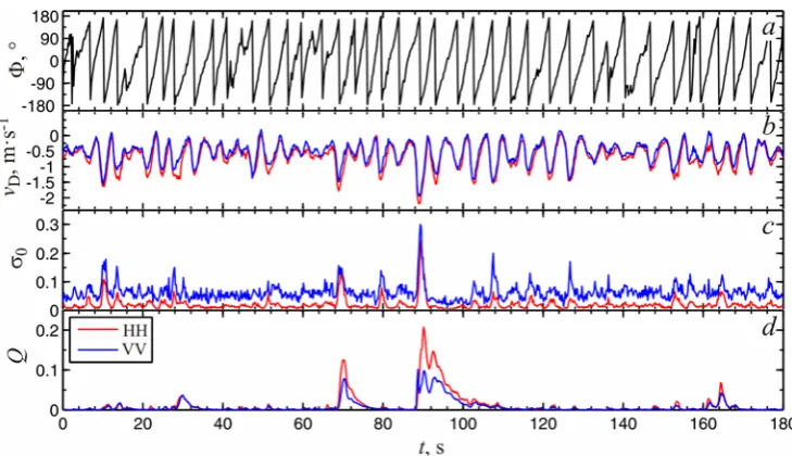
The example of joint processing of video images and radar data is shown in Fig. 2. It is seen that the bursts in Q(t)happen on the long wave specific phase that sufficiently demonstrates the known breaking modulation effect due to the long waves [17]. Therefore exclusion of the wave breaking moments from the sample will provide no opportunity to consider a certain phase of a long wave on which the breakings occur. This, in its turn, will induce decrease or increase of NRCS and the Doppler shifts calculated based on such sampling. In order to avoid it, the sample-average parameters were calculated by a special method.

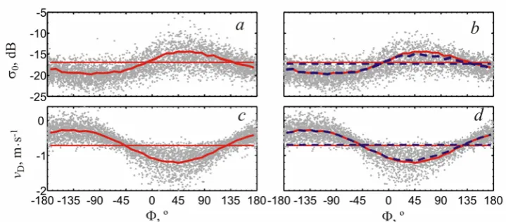
The Doppler frequency shift the variation of which reflects orbital motions of long waves was used for assessing a current phase of the long wave Ф. Depen-dences between the signal parameters and the phase Ф were averaged over the 10-degree intervals that provided the diagram of the signal parameters’ distribution based on the long wave profile. The example of such a distribution is shown in Fig. 3.

Fig. 3. The example of the instantaneous NRCS and the Doppler velocity distributions along the long wave profile on the HH-polarization: a, с – the whole record (red lines); b, d – “the regular surface” (blue lines). Horizontal lines denote average values for all the phases. Observational conditions are the same as on Fig. 2

The described averaging procedure was carried out for all the records and samples from them corresponding to "the normalized surface". In the latter case the average of the diagram differs from the simple arithmetic average calculated for the sample since the long wave phases associated with the breakings are replaced (in-stead of excluding from consideration) by the cases when there are no breakings on this phase.

Results

Contribution of breakings to NRCS.

Comparison of the signal parameters’ average values with those calculated for the samples “the normalized surface” permits to consider the breakings’ contribu-tion to the radar signal. Let us write NRCS of the sea surface in the following form

Q

Q wb

reg

0 σ (1 ) σ

σ = − + ,

where σregis NRCS of the normalized surface and σwbis NRCS of the

breaking-disturbed surface [7].

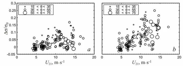
Since Qis a small value and1−Q≈1, the difference ∆σ =σ0−σregcan be

considered to be a component of NRCS related to scattering on the breakings. The breakings’ relative contribution to the total NRCS calculated as ∆σ/σ0 is

shown in Fig. 4 as a function of the wind speed U21. The data are divided into

PHYSICAL OCEANOGRAPHY NO. 4 (2015) 42

42

Fig. 4. Contribution of the wind waves’ breakings to NRCS on the VV-polarization (a) and the HH

-polarization (b) depending on the wind speed

The Doppler velocities of the sea surface without breakings

The scatterer Doppler velocity depends on the scattering mechanism which is primarily conditioned by the incidence angleθ. At smallθ, the scatterer is a sur-face part oriented normally to the radar (specular point) and moving with the phase velocity of the carrying wave. At moderate θ the resonant (Bragg) scattering me-chanism is considered to be dominant. In this case the elementary scatterer is a package consisting of a few periods of the Bragg waves the wave number of which

br

k satisfies the conditionkbr =2krsinθ. The velocity of such a scatterer equals the Bragg waves phase velocity cbr =

(

)

accelera-tion and γ is the surface tension. Along with propagation at their proper velocity, the scatterers are transported by the long waves’ orbital motions non-linearity of which, on the whole, results in the wave (Stokes) surface drift which is a part of the measured surface current velocity. Therefore, the time-averaged instantaneous Doppler velocity represents a sum of the radial component of the surface current velocity Vdrand the Bragg waves’ phase velocitycbr. Consequently, the point of

interest is the difference∆VD=(VD−Vdr) which permits to consider the scatterers’ proper velocities and then – the scattering mechanism.

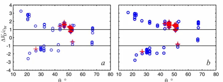
The relation of the measured values ∆VD to the expected Bragg velocity

c

shown in Fig. 5 as a function of the incidence angle at the wind speeds 4 – 12 m·s

-1

. The positive values correspond to the windward azimuths, the negative – the lee ones (in the range 30º from the wind direction). The represented data demonstrate well the contribution of fast specular points at small incidence anglesθ<40°. Fur-ther growth of θleads to decrease of the ratio ∆VD/cbrthough it does not reach

Fig. 5. Relation of the measured values ∆V_D/c_br depending on the incidence angle θ for all the cases (blue symbols) and for the sample “the normalized surface” (red symbols): a – VV-polarization, b –

HH-polarization

The breakings’ contribution to the Doppler velocity can be shown in the same manner as the contribution to NRCS (see above). The values ∆VD/cbr

correspond-ing to the sample “the normalized surface” are shown in Fig. 5 by "+". The number of such points is less than the total number of measurements since the data on the breakings could not always be extracted from the video records because of unsuita-ble conditions of recording. It is seen in Fig. 5 that after the breakings are extracted from the sample, no significant changes in the average instantaneous Doppler ve-locity takes place.

Discussion and conclusions

Analysis of joint radar observations and video records of the sea surface has shown that at the wind speed exceeding 10 m·s -1 in the range of incidence angles 15 – 70º, the contribution of the wind waves’ breakings to the 8 mm wave back-scattering is ~ 5 – 10 % on the VV-polarization and 10 – 30 % on the HH- po-larization.

The developed method of distinguishing passive tracers on the sea surface vid-eo records permitted to determine the surface current velocity in the area of the ra-dar radiation that gave a possibility to analyze the scatterers’ proper velocities. At small incidence angles (θ<40°) the average instantaneous Doppler velocities are practically the same on both polarizations and significantly exceed the Bragg waves’ velocity; it indicates the effect of the specular reflection mechanism. At moderate incidence angles (θ >40°) the Doppler velocity approaches the Bragg one, but at the windward azimuths of observations it can be by 1.5 – 2 times high-er; at that the excess on the HH-polarization is more significant than that on the VV-polarization.

PHYSICAL OCEANOGRAPHY NO. 4 (2015) 44

44

certain roughness on the sea surface which can impact the radio waves’ backscat-tering. Regardless of the scattering mechanism, the micro-breakings’ velocity can be higher than that of the free Bragg waves that can result in overstating of the ob-served Doppler velocity.

On the other hand, the important source of short waves is generation of para-sitic ripple [7, 11]. The phase velocities of the parapara-sitic capillary wave and its car-rier are equal by definition, but it is valid only in the points where the horizontal projection of the carrying wave orbital velocity equals zero. On the other phases, the parasitic ripple is shrink or stretched by the carrier waves’ orbital motions; it leads to broadening the spectrum of the parasitic waves having one and the same phase velocity. Therefore, at the fixed Bragg wave number, the scatterers’ speed related to the parasitic ripples can be either higher or lower than the phase velocity of the free Bragg waves. However, the wave number value of the carrying waves with a higher phase velocity is smaller and, due to the characteristic descending form of the wind waves’ spectrum, their spectral density is higher; hence, they make more significant contribution to the signal as compared to the slower carrying waves. Besides, one of possible mechanisms of increasing the Doppler velocity can consist in spatial modulation of the Bragg ripples by the waves the scale of which does not exceed the illuminated spot size [19].

Summing up the results, we can state that discrepancy between the observed average Doppler velocity and the Bragg waves’ phase velocity can not be ex-plained only by visible breakings of the wind waves. The overstated values of the Doppler velocities can be induced by influence of micro-breakings and parasitic ripples the occurrence of which is, in fact, a specific mechanism of small-scale waves’ breaking.

The authors are grateful to the Professor of the Russian State Hydrometeoro-logical University V.N. Kudryavtsev for valuable remarks and comments.

This work was supported by the Russian Foundation for Basic Research within the framework of the projects 13-05-90912 “mol-in-nr”, 13-05-90429 “ukr-f-a”, 14-45-01559 “r-yug-a" and 14-05-00876, by the Government of Russian Federa-tion in the framework of the grant 11.G34.31.0078, Ministry of educaFedera-tion and science of Russian Federation within the framework of the FTP "Research and de-velopment on priority directions of scientific-technological complex of Russia in 2014 – 2020" (the project unique ID is RFMEFI57714X0110) and partially sup-ported by the grant (the agreement dated August 27, 2013 № 02.V.49.21.0003 be-tween the Ministry of education and science of Russian Federation and the N.I. Lobachevsky State University of Nizhni Novgorod).

REFERENCES

1. Valenzuela, G.R., 1978, “Theories for the interaction of electromagnetic and ocean waves – a review”, Bound. Layer Meteorol., vol. 13, pp. 61-85.

2. Bass, F.G., Fuks, I.M. & Kalmykov, A.I. [et al.], 1968, “Very high frequency radio wave scattering by a disturbed sea surface. Part I: Scattering from a slightly disturbed boundary. Part II: Scattering from an actual sea surface”, IEEE Trans. Antenn. Propagat., vol. 16, no. 5, pp. 554-568.

3. Plant, W.J., 1986, “A two-scale model of short wind-generated waves and scatterometry”, J.

4. Donelan, M.A., Pierson, W., 1987, “Radar scattering and equilibrium ranges in wind-generated waves with application to scatterometry”, J. Geophys. Res. (Oceans), vol. 92, no. C5, pp. 4971-5029.

5. Kalmykov, A.I., Pustovoytenko, V.V. 1976, “On polarization features of radio signals scat-tered from the sea surface at small grazing angles”, J. Geophys. Res. (Oceans and

Atmos-pheres), vol. 81, pp. 1960-1964.

6. Phillips, O.M., 1988, “Radar returns from the sea surface – Bragg scattering and breaking waves”, J. Phys. Oceanogr., vol. 18, pp. 1063-1074.

7. Kudryavtsev, V., Hauser, D. & Caudal, G. [et al.], 2003, “A semiempirical model of the nor-malized radar cross-section of the sea surface 1. Background model”, J. Geophys. Res.

(Oceans), vol. 108, no. C3, pp. FET2-1-FET2-24.

8. Masuko, H., Okamoto, K. & Shimada, M. [et al.], 1986, “Measurement of microwave back-scattering signatures of the ocean surface using X band and Ka band airborne scatterometers”,

J. Geophys. Res. (Oceans),vol. 91, no. C11, pp. 13065-13084.

9. Nekrasov, A., Hoogeboom, P., 2005, “A Ka-Band Backscatter Model Function and an Algo-rithm for Measurement of the Wind Vector Over the Sea Surface”, IEEE Geosci. Rem. Sens.

Lett., vol. 2, no. 1, pp. 23-27.

10. Tanelli, S., Durden, S.L. & Im, E., 2006, “Simultaneous Measurements of Ku- and Ka-Band Sea Surface Cross Sections by an Airborne Radar”, IEEE Geosci. Rem. Sens. Lett., vol. 3, no. 3, pp. 359-363.

11. Ermakov, S.A., Kapustin, I.A. & Sergievskaya, I.A., 2010, “Laboratornoe issledovanie

radi-olokatsionnogo rasseyaniya silno nelineinymi volnami na poverkhnosti vody [Tank study of

radar backscattering from strongly nonlinear water waves]”, Bull. Russ. Acad. Sci. Phys., vol. 74, no. 12, pp. 1695-1698 (in Russian).

12. Hasselmann, K., Raney, R.K. & Plant, W.J. [et al.], 1985, “Theory of synthetic aperture radar ocean imaging: A MARSEN view”, J. Geophys. Res. (Oceans), vol. 90, no. C3, pp. 4659-4686.

13. Plant, W.J., 1989, “The Modulation Transfer Function: Concept and Applications”, Radar

Scattering from Modulated Wind Waves, Netherlands, Springer, pp. 155-172.

14. Kudryavtsev, V., Hauser, D. & Caudal, G. [et al.], 2003, “A semiempirical model of the nor-malized radar cross section of the sea surface 2. Radar modulation transfer function”, J.

Geo-phys. Res. (Oceans), vol. 108, no. C3, pp. FET3-1-FET3-16.

15. Monahan, E.C., Woolf, D.K., 1989, “Comments on “Variations of Whitecap Coverage with Wind stress and Water Temperature”, J. Phys. Oceanogr., vol. 19, pp. 706-709.

16. Mironov, A.S., Dulov, V.A., 2008, “Statisticheskie kharakteristiki sobytiy i dissipatsiya

ener-gii pri obrushenii vetrovykh voln [Statistical properties of individual events and energy

dissi-pation in breaking waves]”, Ekologicheskaya bezopasnost’ pribrezhnoi i shelfovoy zon i

kom-pleksnoe ispol’zovanie resursov shelfa, no. 16, pp. 97-115 (in Russian).

17. Dulov, V.A., Kudryavtsev, V.N. & Bolshakov, A.N., 2002, “A Field Study of White Caps Coverage and its Modulations by Energy Containing Waves”, Gas Transfer at Water Surface,

Geophysical Monograph Series, AGU, vol. 127, pp. 187-192.

18. Babanin, A.V., 2009, “Breaking of ocean surface waves”, Acta Phys. Slov., vol. 59, no. 4, pp. 305-535.