Use of Padé Approximants to
Estimate the Rayleigh Wave
Speed
A. T. Spathis
There exists a range of explicit and approximate solutions to the cubic polynomial Rayleigh equation for the speed of surface waves across an elastic half-space. This article presents an alternative approach that uses Padé approximants to estimate the Rayleigh wave speed with five different approximations derived for two expansions about different points. Maximum relative absolute errors of between 0.34% and 0.00011% occur for the full range of the Poisson ratio from -1 to 0.5. Even smaller errors occur when the Poisson ratio is restricted within a range of 0 to 0.5. For higher-order approximants, the derived expressions for the Rayleigh wave speed are more accurate than previously published solutions, but incur a slight cost in extra arithmetic operations, depending on the desired accuracy.
‡
Introduction
In 1885 Lord Rayleigh published his paper “On Waves Propagated along the Plane Surface of an Elastic Solid” [1] and observed that:
It is proposed to investigate the behavior of waves upon the plane surface of an infinite homogeneous isotropic elastic solid, their character being such that the disturbance is confined to a superficial region, of thickness comparable with the wave-length. ... It is not improbable that the surface waves here investigated play an important part in earthquakes, and in the collision of elastic solids. Diverging in two dimensions only, they must acquire at a great distance from the source a continually increasing preponderance.
real roots of a cubic polynomial whose coefficients are all real and depend on the ratio of the S-wave velocity to the P-wave velocity, or alternatively on the Poisson ratio n of the elastic half-space. He provides the solutions for harmonic waves for both incompressible and compressible half-spaces, shows the elliptic orbit of points on the surface as the wave travels across the surface, demonstrates that the motion is restricted to within approxi-mately one wavelength of the surface, and states that the Poisson ratio may lie between 0.5 and -1 for an elastic material. However, he does not provide explicit expressions for the Rayleigh wave speed.
It appears that the first paper that published explicit expressions for the Rayleigh wave speed for the full range of elastic material properties was by Rahman and Barber [2]. Since that time, a number of authors have sought to develop alternative analytical expres-sions for the Rayleigh wave speed [3–11]. It is noted that the solutions provided cannot be used indiscriminately, as care is required on occasions to choose the correct root to ensure a smooth and continuous estimate of the Rayleigh wave speed [3, 5, 7]. A parallel effort has attempted to derive approximate expressions for the Rayleigh wave speed [3, 12–18].
Complete analytical derivations were provided by [2, 4, 7, 9, 11]. Others have used com-puter algebra to assist in their derivations [3, 5, 6]. The original approach given in [4] con-tains unspecified typographical errors [5, 9]. Indeed, the recent solution given in [9] appears to have been derived earlier and independently but with typographical errors [6]. It has also been shown to be identical to the solution provided in [5]. Cardano’s formula for the roots of a cubic polynomial with real coefficients [19, 20] is used by [2, 5, 7, 9, 11], although the starting point in [9] appears to be different from the other solutions. A more recent solution appears to use Cardano’s formula (but referred to as Shengjin’s formula) [11]. As an aside, an interesting history of Cardano’s formula appears in [21].
Cardano’s formula was published in 1545, and it is perhaps surprising that no explicit solution for the Rayleigh speed was available until the Rahman and Barber publication [2]. It would appear unreasonable to expect that Rayleigh was not aware of the Cardano formula. In any case, and as just one example of prior publication of the Rayleigh wave speed, we may refer to the work in J. E. White’s book, Underground Sound [22]. Given without derivation, and in somewhat standard notation often associated with the use of Cardano’s formula, we find by simple algebra that White’s solution is identical to that of Rahman and Barber. It may be speculated that similar solutions were found even earlier.
The approximate expressions for the Rayleigh wave speed of surface waves have been derived by various methods, including Taylor series expansion of the Rayleigh equation [3], approximation of the Rayleigh equation to lower-degree polynomials using the Lanczos method [13], minimization of the integral of the Rayleigh equation with arbitrary coefficients using a least-squares approach [14], least-squares minimization [15, 18] given a known exact solution [5, 7], use of a bilinear function for the root and applying least squares to determine the coefficients of the bilinear function [16], and an iterative method with asymptotic quadratic convergence [17].
‡
Method of Approximation
Functions may be approximated in various ways. Perhaps the best known is the Taylor series expansion, whereby a function fHzL can be expressed as an infinite series expanded around the point a as
(1) fHzL=‚
k=0
¶ fkHaL k! Hz-aL
k,
where fkHaL is the kth derivative of the function evaluated at the point a. It is usual to
truncate the series to use the lower-order terms as an approximation to the function.
An alternative method to approximate a function is to use Padé approximants. Here the function is approximated as a rational function of two truncated polynomials expanded around the point a:
(2) RHzL= ⁄i=0
m c iHz-aLi
⁄nj=0d
jHz-aLj ,
where the numerator and denominator are polynomials of degree at most m and at most n, respectively. The approximant is referred to as a Padé approximant of type Hm,nL. The approximation given in equation (2) has m+n+1 parameters.
The Rayleigh equation [1] for an elastic half-space is given by
(3) s3-8s2+H24-16LLs-16H1- LL=0,
where s =cR2ëb2, L = b2ëa2, c
R is the Rayleigh wave speed, and a and b are the P-wave and S-P-wave velocities of the medium, respectively. Real roots of equation (3) rep-resent the normalized Rayleigh wave speed, and in the case of several real roots, the smallest is taken. The Poisson ratio may be calculated to give n =H1-2LL ê H2-2LL.
The Padé approximant is found for the left-hand side of equation (3), using computer algebra to calculate the necessary coefficients [23]. Equating the numerator polynomial in equation (2) to zero yields the estimate of the normalized Rayleigh speed. Multiple solu-tions are possible, and these depend on the Padé approximant type, Hm,nL. Given that the Rayleigh equation is a cubic polynomial, the approximations are restricted to m§2 and n§3. In particular, the following Padé approximant types are examined: H1, 1L, H1, 2L,
H1, 3L, H2, 2L, and H2, 3L.
‡
Results
(4) s= ⁄k=0
n+1h
kLk
⁄kn=+01g
kLk
for the type H1,nL. For the types H2, 2L, and H2, 3L, the general expression is
(5) s= ⁄k=0
2 h
kLk+A ⁄k4=0pkLk
⁄kr=0gkLk ,
where r=1 for type H2, 2L and r=2 for type H2, 3L. The coefficient A= -1 for all cases
considered here, except in the single case of type H2, 2L for expansion about 1ë 3 , in which case A=1.
Like the Taylor series expansion, the Padé approximants are expansions about a given value. In the first instance, expansions were obtained around unity, following previous
work [3], but after some trial and error, expansions around 1ë 3 were found to be superior in terms of minimizing the absolute relative error across the full range of values for L. It is worth repeating that the expansions are done for the ratio of the Rayleigh wave speed to the S-wave velocity squared s, unlike the Taylor expansion in Liner [3] that is done about the square root of s. Clearly, it is possible to seek the value around which expansions are minimized using a least-squares approach, some aspects of which are dis-cussed below. Below are shown the results obtained for the coefficients in (4) and (5) for
expansions about 1ë 3 (suitable for the full range of Poisson’s ratio) and 9ê11 (suitable for non-negative Poisson’s ratio), respectively. The coefficient values were obtained using Mathematica 9 and are exact.
The relative absolute errors in percentages for the range of L are shown below for some of the cases considered. The errors are defined as
(6)
D =100 cRn-cRa cRa ,
where Rn and Ra denote numerical and analytical solutions for the Rayleigh wave speed, respectively, and the analytical solution refers to that in [7].
Figure 1 shows a comparison of the exact analytical solution [7], the solution obtained using the Padé approximant H1, 1L, and the solution for a Taylor expansion of the Rayleigh equation given in equation (3). The solution based on the Padé approximant was for an
expansion with a=1ë 3 , while the Taylor series solution was for an expansion with a=1. The relative absolute errors for these two approximate solutions and the one pro-vided by Liner [3] are shown in Figure 2. The Liner solution was a Taylor series expansion in the normalized Rayleigh wave speed, whereas the expansion in its square is shown in Figure 1 and labeled as “Taylor.” It is clear that both Taylor series expansions have increasing errors as L = b2ëa2 increases. The solution based on the Padé
approx-imant H1, 1L has larger errors than either of the Taylor expansion solutions for smaller values of L but performs better for larger values of L.
Figures 3 and 4 show the relative absolute errors for solutions based on the Padé
approxi-mants H1, 2L, H1, 3L and H2, 2L, H2, 3L expanded around the point a=1ë 3 . As expected, the errors are smaller for the solutions based on higher-order Padé approximants.
The following function gives an exact analytical expression for the Rayleigh wave speed [7, 10].
vinhR@L_D:=Module@ 8R, D<,
R=2H27-90L +99L^ 2-32L^ 3L ê27;
D=4H1- LL^ 2H11-62L +107L^ 2-64L^ 3L ê27; Sqrt@
4H1- LL
H2-4Lê3+HR+Sqrt@DDL^H1ê3L+HR-Sqrt@DDL^H1ê3LL^
H-1LD D
The function taylorR gives the Taylor series expansion in the square of the ratio of Rayleigh wave velocity to the S-wave velocity. (The expansion is not in the ratio alone as in the Liner Taylor series expansion given below.)
taylorR@L_D:=Sqrt@H21-16L -Sqrt@141-352L +256L^ 2DL ê10D The function padeR calculates the Rayleigh wave speed based on using Padé approxi-mants. Here mdegree is the numerator degree, ndegree is the denominator degree, avalue is the expansion point, and root1or2 is 1 or 2, so as to ensure the smallest root is chosen. (Normally root1or2 is 1, and an incorrect choice is obvious when over-laying the Rayleigh velocity estimate and the exact analytical Rayleigh wave velocity.)
padeR@L_, mdegree_, ndegree_, avalue_, root1or2_D:=Module@ 8padeExpansion, m<,
padeExpansion=
PadeApproximant@m ^ 3-8 m ^ 2+H24-16LLm-16H1- LL,
8m, avalue, 8mdegree, ndegree<<D;
Sqrt@mê. Solve@Numerator@padeExpansionD==0, mD@@
root1or2DDD D
legName@rspeed_D:=SwitchArspeed, linerR, "Liner",
taylorR, "Taylor", vinhR, "analytical", bergmannR, "Bergmann",
rahMR, "Rahman and Michelitsch",
liRall, "Li full range Poisson ratio", liRpos, "Li positive Poisson ratio",
vinhMR2, RowA9"Vinh and Malischewsky to order ", n2=E, vinhMR3, RowA9"Vinh and Malischewsky to order ", n3=E,
vinhMR4, RowA9"Vinh and Malischewsky to order ", n4=EE
plotRayleighSpeedEstimate is a plotting function that enables comparison of the Rayleigh wave speed obtained by using two functions given in either the body of the report or in the Appendix, and also one derived from a Padé approximant (see the function legName). The input parameters are rspeed1, rspeed2 (for the two different func-tions), and the Padé approximant parameters. Lmax is 3ê4 for the full range of Poisson’s ratio and 1ê2 for positive Poisson’s ratio. Note that when L =0, n =1ê2; L =1ê2,
n =0; L =3ê4, n =–1.
plotRayleighSpeedEstimate@rspeed1_, rspeed2_, mdegree_, ndegree_, avalue_, root1or2_, Lmax_D:=
PlotB 8
rspeed1@xD, rspeed2@xD,
padeR@x, mdegree, ndegree, avalue, root1or2D <,
8x, 0, Lmax<,
ImageSizeØ[email protected], FrameØTrue,
FrameLabelØ:L, CR
b >,
BaseStyleØ8FontSizeØ12<, GridLinesØAutomatic,
GridLinesStyleØDirective@8Dotted<D,
PlotStyleØ88Dashing@8<D, Black<, 8Dashed, Blue<,
8Dashed, Red<<,
PlotLegendsØLineLegend@
8Black, 8Dashed, Blue<, 8Dashed, Red<<,
8
legName@rspeed1D, legName@rspeed2D,
Row@8"Padé H", mdegree, ", ", ndegree, "L, \n",
Style@"a", ItalicD, " = ", TraditionalForm@avalueD<D <,
LabelStyleØ812< D
plotRayleighSpeedEstimate@vinhR, taylorR, 1, 1, 1êSqrt@3D, 1, 3ê4D
0.0 0.1 0.2 0.3 0.4 0.5 0.6 0.7 0.70
0.75 0.80 0.85 0.90 0.95
L
CR b
analytical
Taylor
PadéH1, 1L,
a= 1
3
Ú Figure 1. The normalized Rayleigh wave speed using the Padé approximant H1, 1L expanded around a=1ë 3 and the Taylor series expanded around a=1. The solid curve is the analytical solution given in Vinh and Ogden [7].
We define a function for the approximation to the Rayleigh wave speed given by Liner [3]. The approximation is based on a Taylor series expansion in the ratio of the Rayleigh wave speed to the shear wave speed.
linerR@L_D:=H20-Sqrt@256L^ 2-336L +130DL ê H16L +9L
plot3RayleighWaveSpeedRelativeError is a plotting function for comparing
the relative absolute errors for the Rayleigh speed estimates from two functions and an estimate obtained from a Padé approximant with similar inputs, described above. ymax is the maximum range for the relative error and is adjusted to scale the plot.
plot3RayleighWaveSpeedRelativeError@rspeed1_, rspeed2_, m1_, n1_, a1_, root1or2_, ymax_, Lmax_D:=Module@ 8padeR1<,
padeR1=padeR@L, m1, n1, a1, root1or2D; Plot@
8
100 Abs@Hrspeed1@LD-vinhR@LDL êvinhR@LDD, 100 Abs@Hrspeed2@LD-vinhR@LDL êvinhR@LDD, 100 Abs@HpadeR1-vinhR@LDL êvinhR@LDD <,
8L, 0,Lmax<,
ImageSizeØ[email protected], PlotRangeØ80, ymax<, FrameØTrue,
FrameLabelØ8L, "Relative Absolute Error H%L"<, BaseStyleØ8FontSizeØ12<,
GridLinesØAutomatic,
GridLinesStyleØDirective@8Dotted<D,
PlotStyleØ88Dashing@8<D, Black<, 8Dashed, Blue<,
PlotStyleØ88Dashing@8<D, Black<, 8Dashed, Blue<,
8Dashed, Red<<, PlotLegendsØ
LineLegend@8Black, 8Dashed, Blue<, 8Dashed, Red<<,
8legName@rspeed1D, legName@rspeed2D, Row@8"Padé H", m1, ", ", n1, "L, \n",
Style@"a", ItalicD, " = ", TraditionalForm@a1D<D<, LabelStyleØ812<D
D D
plot3RayleighWaveSpeedRelativeError@linerR, taylorR, 1, 1, 1êSqrt@3D, 1, 0.5, 3ê4D
0.0 0.1 0.2 0.3 0.4 0.5 0.6 0.7 0.0
0.1 0.2 0.3 0.4 0.5
L
Re
la
ti
ve
A
bs
ol
ut
e
E
rror
H
%
L
Liner
Taylor
PadéH1, 1L,
a= 1
3
Ú Figure 2. Relative absolute error for Rayleigh wave speed using the Padé approximant H1, 1L expanded around a=1ë 3 compared to the two Taylor series expansions, both expanded around a=1.
plot2RayleighWaveSpeedRelativeError is a plotting function for comparing
the relative absolute errors for the Rayleigh speed estimates obtained using two Padé approximants. The function has similar inputs described above, and here the suffix 1 or 2 refers to the given Padé approximant.
plot2RayleighWaveSpeedRelativeError@m1_, n1_, a1_, root1or21_, m2_, n2_, a2_, root1or22_, ymax_, Lmax_D:=
Module@
8padeR1, padeR2<,
padeR1=padeR@L, m1, n1, a1, root1or21D; padeR2=padeR@L, m2, n2, a2, root1or22D; Plot@
8
100 Abs@HpadeR1-vinhR@LDL êvinhR@LDD, 100 Abs@HpadeR2-vinhR@LDL êvinhR@LDD <,
8L, 0,Lmax<,
ImageSizeØ[email protected], PlotRangeØ80, ymax<,
PlotRangeØ80, ymax<, FrameØTrue,
FrameLabelØ8"L", "Relative Absolute Error H%L"<, BaseStyleØ8FontSizeØ12<,
GridLinesØAutomatic,
GridLinesStyleØDirective@8Dotted<D,
PlotStyleØ88Dashing@8<D, Black<, 8Dashed, Blue<,
8Dotted, Red<<,
PlotLegendsØLineLegend@
8Black, 8Dashed, Blue<, 8Dotted, Red<<,
8
Row@8"Padé H", m1, ", ", n1, "L, \n",
Style@"a", ItalicD, " = ", TraditionalForm@a1D<D, Row@8"Padé H", m2, ", ", n2, "L, \n",
Style@"a", ItalicD, " = ", TraditionalForm@a2D<D <,
LabelStyleØ812< D
D D
plot2RayleighWaveSpeedRelativeError@1, 2, 1êSqrt@3D, 1, 1, 3, 1êSqrt@3D, 1, 0.05, 3ê4D
0.0 0.1 0.2 0.3 0.4 0.5 0.6 0.7 0.00
0.01 0.02 0.03 0.04 0.05
L
Re
la
ti
ve
A
bs
ol
ut
e
E
rror
H
%
L
PadéH1, 2L,
a= 1
3
PadéH1, 3L,
a= 1
3
plot2RayleighWaveSpeedRelativeError@2, 2, 1êSqrt@3D, 2, 2, 3, 1êSqrt@3D, 1, 0.001, 3ê4D
0.0 0.1 0.2 0.3 0.4 0.5 0.6 0.7 0.0000
0.0002 0.0004 0.0006 0.0008 0.0010
L
Re
la
ti
ve
A
bs
ol
ut
e
E
rror
H
%
L
PadéH2, 2L,
a= 1
3
PadéH2, 3L,
a= 1
3
Ú Figure 4. Relative absolute error for Rayleigh wave speed using the Padé approximants H2, 2L and H2, 3L expanded around a=1ë 3.
It is possible to generate the expressions for equations (4) and (5) based on a Padé approx-imant simply by squaring the Rayleigh wave speed estimate. The square roots of the full set of results given below are good estimates of the Rayleigh wave speed for different ranges of the Poisson ratio. Simple arithmetic yields the results in the forms given in equa-tions (4) and (5).
Here are some useful and accurate expressions for the Rayleigh wave speed squared over
the full range of the Poisson ratio with a=1ë 3 .
padeR@L, 1, 1, 1êSqrt@3D, 1D^ 2
3720-1111 3 -6048L +1168 3 L +2304L2
2J2415-824 3 -2952L +504 3 L +1152L2N
padeR@L, 1, 2, 1êSqrt@3D, 1D^ 2
J2J-197 352+81 671 3 +412 524L
-130 224 3 L -297 216L2+48 384 3 L2+82 944L3NN í
J3J-151 385+63 824 3 +274 296L -82 560 3 L
padeR@L, 1, 3, 1êSqrt@3D, 1D^ 2
J51 643 488-24 481 675 3 -135 469 008L +
54 433 632 3 L +142 200 576L2-41 538 816 3 L2
-74 317 824L3+11 612 160 3 L3+15 925 248L4N í
J3J19 065 399-9 058 928 3 -46 268 016L +
18 278 640 3 L +48 842 496L2-14 146 560 3 L2
-25 104 384L3+3 870 720 3 L3+5 308 416L4NN
padeR@L, 2, 2, 1êSqrt@3D, 2D^ 2
H* note the use of the second root *L 1
12J-768+305 3 -1080L +120 3 LN
J-24 609+7920 3 +4896L -5040 3 L +6912L2+
3 - J107 407 827-48 863 136 3 -223 778 304L +
112 082 400 3 L +81 070 848L2-57 922 560 3 L2+
82 280 448L3-29 859 840 3 L3+15 925 248L4NN
padeR@L, 2, 3, 1êSqrt@3D, 1D^ 2
J49 896-23 181 3 +44 280L +3936 3 L -48 384L2+6912 3 L2
-3 - J700 775 058-385 572 656 3 -626 722 704L +435 009 168
3 L -1 025 213 760L2+514 432 512 3 L2+735 215 616L3
-685 559 808 3 L3+1 066 991 616L4-254 803 968 3 L4NN í
J3J4695-2752 3 +19 152L -4320 3 L +2304L2NN
Here are some useful and accurate expressions for the Rayleigh wave speed squared over the positive range of Poisson’s ratio with a=9ê11.
padeR@L, 1, 1, 9ê11, 1D^ 2
23 567 547-61 411 856L +41 229 056L2
padeR@L, 1, 2, 9ê11, 1D^ 2
I2I-8 842 983 329+34 001 548 372L
-44 609 838 592L2+19 954 863 104L3MM ë
I11I-1 761 755 777+6 547 138 664L -8 337 639 552L2+
3 628 156 928L3MM
padeR@L, 1, 3, 9ê11, 1D^ 2
I53 083 060 316 861-269 891 481 763 024L +524 274 245 766 656L2
-460 797 698 797 568L3+154 530 459 877 376L4M ë
I11I5 287 767 311 575-26 203 829 630 176L +49 730 715 981 056L2
-42 768 713 867 264L3+14 048 223 625 216L4MM
padeR@L, 2, 2, 9ê11, 1D^ 2
1
132H6309+38 720LLI3 959 227+3 266 032L -3 748 096L
2
-, I10 234 921 221 073-8 321 453 581 408L -17 637 748 927 744L2+
13 830 534 209 536L3+14 048 223 625 216L4MM
padeR@L, 2, 3, 9ê11, 1D^ 2
J19 181 891+283 369 416L -187 404 800L2- 122
, I6 849 361 706 093+61 917 473 544 432L +41 767 161 240 992L2
-430 404 628 211 712L3+428 470 820 569 088L4MN í
I11I-968 761+15 087 248L +3 748 096L2MM
‡
Discussion
Polynomial expressions for the Rayleigh wave speed are given in equations (4) and (5) with respective coefficients given above. These expressions have been derived using Padé
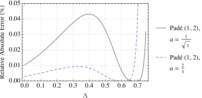
approximants around a=1ë 3 and a=9ê11 for 0§ L §0.75 (Poisson ratio in the range 0.5 to -1) and 0§ L §0.5 (Poisson ratio in the range 0.5 to 0), respectively. The two expansion values (a in equations (1) and (2)) were obtained by examining the area under the relative absolute error curve for increments of a between 0.5 and 1. In principle, a least-squares solution for the value of a producing the minimum error would be feasible for each Padé type, but in so doing we ignore the detailed shape of the error curve across the range of L values. For example, Figure 5 shows the relative absolute error for the
Rayleigh wave speed based on Padé type H1, 2L for expansions around a=1ë 3 and a=2ê3. While the error is less for the expansion around a=2ê3 for most of the range of
L values, we observe that for larger values of L, the errors become larger and exceed
those for the expansion around a=1ë 3 . This basic behavior is characteristic of the errors obtained (but not shown) using the Padé types H1, 1L and H1, 3L. It is worth noting that for non-negative Poisson’s ratio of 0§ L §0.5, the errors are smaller for expansions about a=2ê3 for the three Padé types H1, 1L, H1, 2L, and H1, 3L. The question arises, is it possible to expand around another value that will have smaller errors for non-negative Poisson’s ratio? Figure 6 shows the relative absolute error for the Padé type H1, 2L
expanded about a=2ê3 and a=7ê8. The error in the latter case is smaller for all values up to approximately L>0 .47, after which it increases beyond that for the expansion about a=2ê3, but not significantly. The maximum error is about the same for both cases. Once more, similar behavior is observed for the other two Padé types H1, 1L and H1, 3L.
Figure 7 shows the relative absolute errors for the Rayleigh wave speed based on using
the Padé type H2, 3L expanded around a=1ë 3 and a=2ê3. The behavior of these curves is different from those shown earlier—here there is a monotonic decrease in the error for most of the full range of L as it increases. The errors are one hundred times smaller than those based on the Padé type H1, 2L shown in Figure 6. A somewhat extraor-dinary reduction of a further five times (so a total of a 500-fold reduction) in relative absolute error occurs for the Rayleigh wave speed estimate based on the Padé type H2, 3L
expanded around a=9ê11 and shown in Figure 8.
plot2RayleighWaveSpeedRelativeError@1, 2, 1êSqrt@3D, 1, 1, 2, 2ê3, 1, 0.05, 3ê4D
0.0 0.1 0.2 0.3 0.4 0.5 0.6 0.7 0.00
0.01 0.02 0.03 0.04 0.05
L
Re
la
ti
ve
A
bs
ol
ut
e
E
rror
H
%
L
PadéH1, 2L,
a= 1
3
PadéH1, 2L,
a= 2
3
Ú Figure 5. Relative absolute error for Rayleigh wave speed using the Padé approximants H1, 2L expanded around the points a=1ë 3 and a=2ê3.
plot2RayleighWaveSpeedRelativeError@1, 2, 2ê3, 1, 1, 2, 7ê8, 1, 0.02, 1ê2D
0.0 0.1 0.2 0.3 0.4 0.5
0.000 0.005 0.010 0.015 0.020
L
Re
la
ti
ve
A
bs
ol
ut
e
E
rror
H
%
L
PadéH1, 2L, a= 2
3
PadéH1, 2L, a= 7
8
Ú Figure 6. Relative absolute error for Rayleigh wave speed using the Padé approximants H1, 2L expanded around the points a=2ê3 and a=7ê8.
plot2RayleighWaveSpeedRelativeError@2, 3, 1êSqrt@3D, 1, 2, 3, 2ê3, 1, 0.0002, 3ê4D
0.0 0.1 0.2 0.3 0.4 0.5 0.6 0.7 0.00000
0.00005 0.00010 0.00015 0.00020
L
Re
la
ti
ve
A
bs
ol
ut
e
E
rror
H
%
L
PadéH2, 3L,
a= 1
3
PadéH2, 3L, a= 2
3
plot1RayleighWaveSpeedRelativeError is a plotting function for the relative absolute error of the Rayleigh speed obtained using a single Padé approximant. The function has similar inputs described earlier.
plot1RayleighWaveSpeedRelativeError@m1_, n1_, a1_, root1or2_, ymax_, Lmax_D:=Module@
8padeR1<,
padeR1=padeR@L, m1, n1, a1, root1or2D; Plot@
100 Abs@HpadeR1-vinhR@LDL êvinhR@LDD,
8L, 0,Lmax<,
ImageSizeØ[email protected], PlotRangeØ80, ymax<, FrameØTrue,
FrameLabelØ8L, "Relative Absolute Error H%L"<, BaseStyleØ8FontSizeØ12<,
GridLinesØAutomatic,
GridLinesStyleØDirective@8Dotted<D,
PlotStyleØ88Dashing@8<D, Black<, 8Dashed, Blue<,
8Dotted, Red<<,
PlotLegendsØLineLegend@
8Black, 8Dashed, Blue<, 8Dotted, Red<<,
8Row@8"Padé H", m1, ", ", n1, "L, \n",
Style@"a", ItalicD, " = ", TraditionalForm@a1D<D<, LabelStyleØ812<
D D D
plot1RayleighWaveSpeedRelativeError@2, 3, 9ê11, 1, 0.00000012, 1ê2D
0.0 0.1 0.2 0.3 0.4 0.5
0 2.µ10-8 4.µ10-8 6.µ10-8 8.µ10-8 1.µ10-7 1.2µ10-7
L
Re
la
ti
ve
A
bs
ol
ut
e
E
rror
H
%
L
PadéH2, 3L,
a= 9
11
It is worth summarizing the various error estimates arising from the Rayleigh wave speed based on the Padé approximant types studied for the two ranges of Poisson’s ratios (Table 1). These are compared to other published estimates given in Table 2. Tables 1 and 2 show this data and also the number of arithmetic operations required to compute the value of s (equation (3)), from which we estimate any given Rayleigh wave speed. The latter information shows the tradeoff between the accuracy of the Rayleigh wave speed estimate and the associated computational effort. The operations included are addition, subtraction, multiplication, division, and the taking of a root or a trigonometric function; raising to a power is taken as a series of multiplications, and the minimum number of such operations is used wherever possible. It is assumed that an analytical solution is exact, that L is known, and that for each approximate solution all coefficients are known and retained as integers until the calculation commences. In the case of the exact solution based on Car-dano’s formula, two different expressions exist for different values of L, and in this case, the number of operations is given for each path separated by a forward slash. Functions not previously introduced in the body of the text and required to calculate the estimates in Table 2 may be found in the Appendix.
The data in Tables 1 and 2 shows that the computational effort is generally greatest for the three analytical solutions. The approximate solutions based on the Padé approximants improve their error estimates approximately tenfold as we move from Padé types H1, 1L to
H2, 3L for expansions around a=1ë 3 . The number of arithmetic operations increases by about five for Padé types H1, 1L to H1, 3L, without a significant change in the number of operations as we move to Padé types H2, 2L and H2, 3L. For the Padé types expanded around a=9ê11 and for non-negative Poisson’s ratio, we find a remarkable reduction in the errors, commencing with a thirtyfold reduction in the Padé type H1, 1L, followed by a twentyfold reduction as we move from Padé types H1, 1L to H1, 3L, and a further tenfold reduction in the errors as we move to Padé types H2, 2L to H2, 3L. The Padé type H1, 1L
Padé type a=1
,3
0§ L §0.75
a=9ê11
0§ L §0.5
Number of arithmetic operations
H1, 1L 0.34 0.011 9
H1, 2L 0.044 0.0005 15
H1, 3L 0.0057 0.000023 20
H2, 2L 0.00076 1.9µ10-6 19 H2, 3L 0.00011 1.1µ10-7 21
Ú Table 1. Maximum relative absolute error (%) and number of arithmetic operations for the Rayleigh wave speed estimates based on Padé approximants.
Method unless noted otherwise0§ L §0.5 Number of arithmeticoperations
Exact@2, 22D none 21 or 26Hsee textL
Exact@5, 7D none 36
Exact@9D none 25
Bergmann@24D 0.47 3
Taylor expansion for,s@3D 0.29 10 Taylor expansion 0.17 10 Lanczos method@13D 0.38 13 Lanczos method@13D 0.43H0§ L §0.75L 13 Least squares on integral of cubic@14D 0.004 13 Least squares on integral of cubic@14D 0.16H0§ L §0.75L 13
Least squares for quadratic equation inn@18D
0.014 5
Least squares for cubic equation inn@18D
0.0031 8
Least squares for quartic equation inn@18D
0.000051 11
‡
Conclusion
The Rayleigh wave speed was estimated based on expansions of the Rayleigh equation by Padé approximants and equating the numerator of that representation to zero. The numerator polynomials were solved for the normalized Rayleigh wave speed and provide five distinct solutions. The solutions have varying degrees of accuracy, depending on the value about which the Rayleigh equation is expanded. Good, accurate solutions occur for the full range of Poisson’s ratio, and even more accurate solutions are found for non-neg-ative Poisson’s ratio. It is concluded that these expressions for the Rayleigh wave speed provide a useful approximation, with a balance between accuracy and number of arith-metic operations required.
‡
Appendix
This Appendix contains a number of functions that estimate the Rayleigh wave speed, which may be used to reproduce some results for the approximate solutions found in Table 2. Other needed functions have been presented in the body of the main text.
Here is the Bergmann formula from Vinh and Malischewsky [24].
bergmannR@L_D:=Module@ 8n<,
n =H2L -1L ê H2HL -1LL;
H0.87+1.12nL ê H1+ nL D
Here is the Vinh and Malischewsky [18] formula to degree 2 in Poisson’s ratio.
vinhMR2@L_D:=Module@ 8n<,
n =H2L -1L ê H2HL -1LL; 0.8739+0.2008n -0.07566n^ 2
D
Here is the Vinh and Malischewsky [18] formula to degree 3 in Poisson’s ratio.
vinhMR3@L_D:=Module@ 8n<,
n =H2L -1L ê H2HL -1LL;
0.874006+0.19704n -0.05558n^ 2-0.02677n^ 3
Here is the Vinh and Malischewsky [18] formula to degree 4 in Poisson’s ratio.
vinhMR4@L_D:=Module@ 8n<,
n =H2L -1L ê H2HL -1LL;
0.8740325+0.1953777n -0.038923n^ 2-0.080072n^ 3+
0.053299n^ 4
D
Here is the Rahman and Michelitsch [18] formula using the Lanczos approximation.
rahMR@L_D:=Module@ 8n<,
n =H2L -1L ê H2HL -1LL; Sqrt@
H30.876-14.876n
[email protected]^ 2 -93.122752n +124.577376LDL ê H26H1- nLLD
D
Here is the Li [14] formula for the full range of Poisson’s ratio.
liRall@L_D:=Module@ 8n<,
n =H2L -1L ê H2HL -1LL; Sqrt@
H28.84-12.84n - [email protected]^ 2 -66.98n +124.1LDL ê H23.18H1- nLLD
D
Here is the Li [14] formula for the positive range of Poisson’s ratio.
liRpos@L_D:=Module@ 8n<,
n =H2L -1L ê H2HL -1LL; Sqrt@
H27.425-11.425n
[email protected]^ 2 -52.4769n +121.0384LDL ê H21.5H1- nLLD
‡
References
[1] L. Rayleigh, “On Waves Propagated along the Plane Surface of an Elastic Solid,” Pro-ceedings of the London Mathematical Society, S1-17(1), 1885 pp. 4–11.
doi:10.1112/plms/s1-17.1.4.
[2] M. Rahman and J. R. Barber, “Exact Expressions for the Roots of the Secular Equation for Rayleigh Waves,” Journal of Applied Mechanics, 62(1), 1995 pp. 250–252.
doi:10.1115/1.2895917.
[3] C. L. Liner, “Rayleigh Wave Approximations,” Journal of Seismic Exploration, 3, 1994 pp. 273–281.
[4] D. Nkemzi, “A New Formula for the Velocity of Rayleigh Waves,” Wave Motion, 26(2), 1997 pp. 199–205. doi:10.1016/S0165-2125(97)00004-8.
[5] P. G. Malischewsky, “Comment to ʻA New Formula for the Velocity of Rayleigh Wavesʼ by D. Nkemzi [Wave Motion 26 (1997) 199–205],” Wave Motion, 31(1), 2000 pp. 93–96. doi:10.1016/S0165-2125(99)00025-6.
[6] H. Mechkour, “The Exact Expressions for the Roots of Rayleigh Wave Equation,” Pro-ceedings of the 2nd International Colloquium of Mathematics in Engineering and Numerical Physics (MENP-2), Bucharest, 2002, Geometry Balkan Press, 2003 pp. 96–104.
[7] P. C. Vinh and R. W. Ogden, “On Formulas for the Rayleigh Wave Speed,” Wave Motion,
39(3), 2004 pp. 191–197. doi:10.1016/j.wavemoti.2003.08.004.
[8] P. G. Malischewsky Auning, “ A Note on Rayleigh-Wave Velocities as a Function of the Material Parameters,” Geofísica internacional, 43(3), 2004 pp. 507–509.
www.geofisica.unam.mx/unid_apoyo/editorial/publicaciones/investigacion/ geofisica_internacional/anteriores/2004/03/Malischewsky.pdf.
[9] D. W. Nkemzi, “A Simple and Explicit Algebraic Expression for the Rayleigh Wave Velocity,”
Mechanical Research Communications, 35(3), 2008 pp. 201–205. doi:10.1016/j.mechrescom.2007.10.005.
[10] P. G. Malischewsky, “Reply to Nkemzi, D. W., ʻA Simple and Explicit Algebraic Expression for the Rayleigh Wave Velocity,ʼ [Mechanical Research Communications (2007), doi:10.1016/j.mechrescom.2007.10.005],” Mechanical Research Communications, 35(6), 2008 p. 428. doi:10.1016/j.mechrescom.2008.01.011.
[11] X.-F. Liu and Y.-H. Fan, “A New Formula for the Rayleigh Wave Velocity,” Advanced Mate-rials Research, 452–453, 2012 pp. 233–237.
[12] D. Royer, “A Study of the Secular Equation for Rayleigh Waves Using the Root Locus Method,” Ultrasonics, 39(3), 2001 pp. 223–225. doi:10.1016/S0041-624X(00)00063-9.
[13] M. Rahman and T. Michelitsch, “A Note on the Formula for the Rayleigh Wave Speed,”
Wave Motion, 43(3), 2006 pp. 272–276. doi:10.1016/j.wavemoti.2005.10.002.
[14] X.-F. Li, “On Approximate Analytic Expressions for the Velocity of Rayleigh Waves,” Wave Motion, 44(2), 2006 pp. 120–127. doi:10.1016/j.wavemoti.2006.07.003.
[15] P. C. Vinh and P. G. Malischewsky, “Explanation for Malischewskyʼs Approximate Expression for the Rayleigh Wave Velocity,” Ultrasonics, 45(1–4), 2006 pp. 77–81.
doi:10.1016/j.ultras.2006.07.001.
[16] D. Royer and D. Clorennec, “An Improved Approximation for the Rayleigh Wave Equation,”
Ultrasonics, 46(1), 2007 pp. 23–24. doi:10.1016/j.ultras.2006.09.006.
[17] A. V. Pichugin. “Approximation of the Rayleigh Wave Speed.” (Jan 10, 2008) people.brunel.ac.uk/~mastaap/draft06rayleigh.pdf.
[18] P. C. Vinh and P. G. Malischewsky, “Improved Approximations of the Rayleigh Wave Velocity,” Journal of Thermoplastic Composite Materials, 21(4), 2008 pp. 337–352.
[19] M. Abramowitz and I. A. Segun, eds., Handbook of Mathematical Functions, New York: Dover Publications, 1965.
[20] D. Zwillenger, ed., Standard Mathematical Tables and Formulae, 31st ed., Boca Raton: CRC Press, 2003.
[21] P. R. Hewitt. “Cardanoʼs Formulas or a Pivotal Moment in the History of Algebra.” (Apr 7, 2009) livetoad.org/Courses/Documents/bb63/Notes/cardanos_formulas.pdf.
[22] J. E. White, Underground Sound: Application of Seismic Waves, New York: Elsevier, 1983.
[23] Mathematica, Release Version 9.0, Champaign: Wolfram Research, Inc., 2013.
[24] P. C. Vinh and P. G. Malischewsky, “An Approach for Obtaining Approximate Formulas for the Rayleigh Wave Velocity,” Wave Motion, 44(7–8), 2007 pp. 549–562.
doi:10.1016/j.wavemoti.2007.02.001.
A. T. Spathis, “Use of Padé Approximants to Estimate the Rayleigh Wave Speed,” The Mathematica Journal, 2015. dx.doi.org/doi:10.3888/tmj.17-1.
About the Author
A. T. (Alex) Spathis works in rock mechanics and rock dynamics. He has measured the stresses in the Earth’s crust at shallow depths of tens of meters down to moderate depths of over 1000 meters. This data assists in understanding earthquakes and in the design of safe underground mines. He has formal qualifications in applied mathematics, electrical engineering, and rock mechanics, and has a Ph.D. in geophysics.
A. T. Spathis
Orica Technical Centre PO Box 196
Kurri Kurri NSW Australia 2327