Derivative Free Multilevel Optimization

(1)

DERIVATIVE FREE MULTILEVEL OPTIMIZATION

B. KARAS ¨OZEN1, §

Abstract. Optimization problems with different levels arise by discretization of ordi-nary and partial differential equations. We present a trust-region based derivative-free multilevel optimization algorithm. The performance of the algorithm is shown on a shape optimization problem and global convergence to the first order critical point is proved.

Keywords: Derivative-free optimization; multilevel optimization; shape optimization; trust-region methods.

AMS Subject Classiﬁcation: 90C30, 65K05, 90C26, 90C06, 90C56 ; 65D05.

1. Introduction

Discretization of infinite dimensional optimization problems, such as optimal control problems with partial differential equations(PDEs) lead to large-scale finite dimensional optimization problems. This kind of problems can be solved for a dicretization level by the existing large scale numerical optimization packages. But this approach does not exploit the structure of the underlying infinite dimensional optimization problem which can be dicretized at different levels. There exist several methods, which make use of the discretization of infinite dimensional problems at different levels. The simplest approach is to use coarse grids in order to compute approximate solutions for the starting points on a finer grid. Efficient optimizations methods were developed recently within the framework of multi-grid methods [2, 11, 13]. In [11], a recursive line-search based truncated Newton method was developed for efficient solution of large-scale convex optimization problems arising from the discretization of partial differential equations (PDEs). This approach is then extended to nonconvex problems using the trust-region approach in a series of papers [7, 8, 9, 17], known as recursive multilevel (multiscale) trust-region (RMTR) methods. The recursive multilevel optimization methods use a model of the objective function on the coarse grid at the lower level for optimization on the fine grid at the higher level .

For continuously diﬀerentiable functions usually gradient based methods are used the ﬁnd the local minimum of the objective function. However, for many practical problems the derivatives of the objective function are either not available or costly to evaluate. Derivative free optimization methods build models of function based on sample func-tion value or directly exploit a sample set of funcfunc-tion values without building an explicit model [6, 10]. Among them are the well known trust-region based methods by modeling

1

Department of Mathematics & Institute of Applied Mathematics, Middle East Technical University, Ankara, Turkey.

e-mail: [email protected];

§ Manuscript received: March 01, 2014.

(2)

the objective function by multivariate interpolation in combination with the trust-region techniques [3, 4, 5].

In this paper we have developed a trust-region based derivative-free recursive multi-level optimization (DFRMTR) method for solving the ﬁnite-dimensional optimization problem at diﬀerent levels. In the next section, the DFRMTR algorithm is described. In Section 3 we show the implementation of our algorithm for a shape optimization problem and the convergence analysis of the method is given in Section 4.

2. Derivative free multilevel optimization

Consider the problem

min

x∈Rn f(x), (1)

where f : Rn _→ _R _{is a smooth function and bounded below.} _{Trust-region methods} compute a sequence of iterates xk, starting from an initial guess x0, converging to the solution of the problem (1). At each iteration k, a linear or quadratic model Qk of f is constructed in the neighborhood of the current iteratexk,Bk={xk+s:s∈Rnand ||s|| ≤ ∆k}, with the trust-region radius ∆k, here || · || represents the Euclidean norm. At the kth step, the model function within the trust-regionBk, is given as

Qk(xk+s) =Qk(xk) +< s, gk>+1

2 < s, Hks > (2) for some g ∈ Rn and some symmetric n×n matrix H, where <·,·> denotes the inner product . The vector g and the matrix H do not necessarily correspond to the ﬁrst and second derivatives of the objective functionf. They are determined by requiring that the model (2) interpolates the function f at a set Y = {yi} of points containing the current iteratexk,f(yi) =mk(yi) for allyi ∈Y. Here,Y denotes the set of interpolation points, which is a subset of the set of points at which the values off is known, including the cur-rent iterate. Building the full quadratic model in (2) requires the determination off(xk), the components of the vectorgk and the entries of the matrixHk; so that the cardinality ofY must be equal top= 1₂(n+ 1)(n+ 2).

At each iteration stepk the trust-region subproblem deﬁningsk

min s∈B(0;∆k)

Qk(xk+s), (3)

has to be solved. where B(0; ∆k) is the trust-region of radius ∆k centered at 0 and s=x−xk.

(3)

We construct the lower model hi based onQi−1 which results from the interpolation of f(x) at the leveli−1, similar to the recursive multilevel optimization methods in [7, 9, 17]. The lower level model is deﬁned as

hi,k(xi,k) =Qi−1(xi,k) + (∇Qi,k(xmin)− ∇Qi−1,k(xmin))T(xi,k−xmin), (4) where xmin is the minimum of value of f(x) at the (i−1)th level and Qi₋1 is a fixed function for every iterationkatith level. In the derivative-free case, the prolongation and restriction operators can not be used, because the gradient and Hessian of the functionf(x) are not available. Instead of this, we use either the minimum point in the interpolation set of (i−1)th level to construct the new interpolation set at the level i, or we take the interpolation set from the previous level i−1. In the following, i (1 ≤ i ≤ r) denotes the level index and the k, the the current iteration at the level i. The lower level model corresponds to the modification of the modelQi₋1 ati’th level. The lower level model can not always be useful since∇Qi−1,k can be close to zero with respect to∇Qi,k. In this case the current iterate appears to be first-order critical for (i−1)th level while it is not for i’th level. Therefore the lower model is useful only if∇Qi−1,k is large enough compared to

∇Qi,k and ∇Qi,k is greater than a constantϵQ, which is given by the following condition (see also [7, 9, 17]):

∥∇Qi,k∥ ≥κQ∥∇Qi−1,k∥ and ∥∇Qi,k∥ ≥ϵQ, where κQ, ϵQ∈(0,1). (5) When the conditions above are satisﬁed, for kth iteration at the ith level the lower level modelhi,k is used and the trust-region subproblem becomes

min

∥si,k∥≤∆i,k

hi,k(xmin+si,k) (6) wheresi,k =xi,k−xmin.

Otherwise, the model (2) is used and trust-region subproblem at the Taylor step becomes

min

∥si,k∥≤∆i,k

Qi,k(xi,k+si,k) +∇Qi,k(xi,k+si,k)Tsi,k+sTi,k∇2Qi,k(xi,k+si,k)si,k. (7) We can now deﬁne the derivative-free multilevel optimization (DFRMTR) algorithm.

Step 0: Initialization

Given x0 ∈ Rn, the initial guess, ∆0, the initial trust-region radius, construct a well-poised interpolation setY around x0 _∈_Y _⊂_Rn _{within the initial trust-region. and build} the quadratic interpolation modelQi on the interpolation set Y.

Step 1: Model Choice

If i= 1 or if the conditions: ∥∇Qi∥ ≥κQ∥∇Qi₋1∥ and ∥∇Qi∥> ϵQ fail, go to Step 3 (Taylor step), otherwise go to Step 2 (lower level model).

Step 2: Lower level model computation

Solve the trust-region subproblem min

∥s∥<∆i,k

hi,k(xmin+s).

(4)

Solve the model problem

min

∥s∥≤∆i,k

Qi(x) +∇QT_i,k(x)s+1 2s

T_∇2_Qi,k_(x)s.

Step 4: Updating the interpolation set

Compute the ratio

ρi,k = (fi(xk)−fi(ˆxk))/δi,k, with ˆxk= ˆxi,k =xi,k+si,k,

• δi,k =Qi(xk)−Qi(ˆxk) (if the model (2) is used),

• δi,k =hi(xk)−hi(ˆxk) (if the lower level model is used).

• Successful step: If ρi,k ≥ η0, include ˆxk in Y by dropping one of the existing interpolation points.

• Unsuccessful step: Ifρi,k < η0andY is inadequate inx∈ Bk, improve the geometry of the interpolation set.

Step 5: Updating the current iterate

Determine ¯xkwith the best objective function valuef(¯xk) = min xj∈Y,xj̸=xk

f(xj). If the

im-provement is suﬃcient ¯ρi,k = (fi(xk)−fi(¯xk))δi,k ≥η0, setxk+1= ¯xk, otherwisexk+1=xk wherexk=xi,k.

Step 6: Trust-region radius update

• ifρi,k ≥η1, increase the trust-region radius, ∆i,k+1∈[∆i,k, γ2∆i,k]

• ifρi,k < η0and the cardinality ofY∩Bkwas less thann+1 when ˆxkwas computed, reduce the trust-region radius, ∆i,k+1∈[γ0∆i,k, γ1∆i,k+1]

• otherwise set ∆i,k+1= ∆i,k.

Step 7: Termination

The algorithm is terminated when one of the following three criteria are satisﬁed:

• The radius of trust-region is small enough, such that. ∆≤ϵ∆

• Final interpolation point set has the ‘ good geometry’ property.

• Maximum function evaluations or number of maximum iterations are reached. Incrementkby one and go to Step 0.

In the algorithm, some constants and parameters are used: ϵ∆ denotes the minimum value for the trust-region radius, 0 < η0 < η1 < 1 are parameters to improve quality of interpolation set, 0 < γ0 ≤ γ1 < γ2 ≤ 1 are constant which monitor the trust-region radius, κQ ∈ (0,1) is a constant which is used for the model choice, ϵQ ∈ (0,1) is the tolerance for the gradient norm andϵf un is the tolerance for the function reduction.

(5)

subproblem for the lower level problem (6) is solved by CONDOR using the Mor´e and Sorensen algorithm [12]. For solution of the trust-region subproblem (7) withe DFO, we use either, trust with the full eigenvalue decomposition, based on the secular equation

1 ∆ −

1

∥s∥ = 0 [16] or lmlib or the Levenberg-Marquardt algorithm with the Mor´e and Sorensen technique. Updating and improving the interpolation set are explained in detail in [3, 4] and they are implemented in diﬀerent ways in the DFO and CONDOR. The geometry of the interpolation set has to maintained at every iteration. There must be at leastn+ 1 points are in the trust-region. If there are less than n+ 1 points, the farthest point from the current trust-region center by ˜x is replaced with a point on the boundary of the current trust-region, so that the interpolation set is well poised [3, 4].

3. Numerical Example

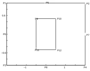
We consider a shape optimization problem over a rectangular region with a rectangular hole Ω(u) parameterized with the coordinatesu= (P9, P12), as in Figure 1.

min 1 2

∫

Ω(u)

(y(x1, x2)−yd)2dx such that

∆y= 1 in Ω(u), y= 0 on ∂Ω(u).

Here, y(x1, x2) is a state variable, yd is the desired state, and u is the control variable. Dataydis designed in such a way, thaty(u∗) is the global minimum for the optimal control u∗.

−1 P8 1 P4 P3

−0.6 P6 0.6

P1 P5 P2

P7 P9 P10

P11 P12

Figure 1. Shape optimization problem

We have used the parameters as in the MATLAB version of the DFO algorithm [15]:

ϵtrust = 0.01, ϵdet= 1e−12,∆0= 0.2, η0= 0.45, η1 = 0.75, γ1 = 0.3, γ2= 1, ϵdist= 0.001, ϵf un= 1e−8, κQ = 0.01, ϵQ= 0.001.

In CONDOR [1] only the parameters ρstart = 0.2, the initial distance between sample points, and ρend = 0.001 stopping criteria for the distance of the points, can be speciﬁed by the user and other parameters are ﬁxed.

The initial trust-region radius was taken as ∆0 = 0.2 and ϵf un = 1.0e−8. In all compu-tations, we use u0 = [−0.5,0.5,0.5,−0.5]T as starting value for the control variable and ¯

u denotes the optimal control computed at the point (P9, P12). The exact value of the optimal control is not known.

(6)

Tables 1 and 2, we see that CONDOR requires smaller number of function evaluations and it gives more accurate results for the minimization of the cost function than the DFO.

Table 1. DFO without multilevel derivative-free optimization

level # iterations # func. eval. func. value u¯

1 32 103 5.0677e-008 −0.7108,0.2386,−0.1397,−0.2385 2 35 91 1.1911e-010 −0.7501,0.2499,−0.2499,−0.2499 3 39 82 9.4293e-009 −0.7504,0.2498,−0.2491,−0.2495 4 33 84 1.0900e-008 −0.7501,0.2495,−0.2485,−0.2499 5 35 75 5.0694e-011 −0.7500,0.2500,−0.2501,−0.2500

Table 2. CONDOR without multilevel derivative-free optimization

level # func. eval. # func. value u¯

1 131 3.0482e-014 −0.7158,0.2275,−0.0894,−0.2275 2 82 3.2440e-014 −0.7500,0.2500,−0.2500,−0.2500 3 60 1.0045e-012 −0.7500,0.2500,−0.2500,−0.2500 4 52 1.6304e-011 −0.7500,0.2500,−0.2500,−0.2500 5 61 2.8944e-012 −0.7500,0.2500,−0.2500,−0.2500

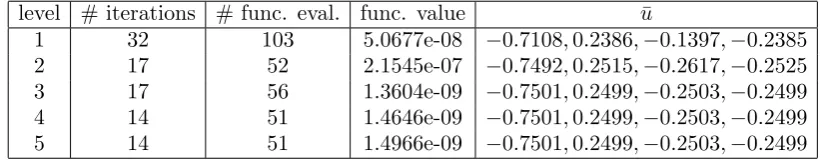
In Tables 3 and 4, the numerical results obtained with the DFRMTR algorithm are shown. The interpolation set of Qi is constructed by using the minimum point of the (i−1)th level. The trust-region subproblem is solved bylmlib ortrust routines.

Table 3. DFRMTR with lmlib

level # iterations # func. eval. # func. value u¯

1 32 103 5.0677e-08 −0.7108,0.2386,−0.1397,−0.2385 2 17 52 2.1545e-07 −0.7492,0.2515,−0.2617,−0.2525 3 17 56 1.3604e-09 −0.7501,0.2499,−0.2503,−0.2499 4 14 51 1.4646e-09 −0.7501,0.2499,−0.2503,−0.2499 5 14 51 1.4966e-09 −0.7501,0.2499,−0.2503,−0.2499

Table 4. DFRMTR with trust

level # iterations # func. eval. # func. value u¯

(7)

In Tables 4 and 5, the numerical results are given by constructing the initial interpo-lation set of Qi by using last interpolation set of previous (i−1)th level with lmlib and trust routines.

Table 5. DFRMTR with lmlib

1 32 103 5.0677e-08 −0.7108,0.2386,−0.1397,−0.2385 2 21 49 4.9240e-09 −0.7493,0.2500,−0.2492,−0.2499 3 5 21 1.3604e-09 −0.7493,0.2500,−0.2492,−0.2499 4 4 19 9.3654e-09 −0.7493,0.2500,−0.2492,−0.2499 5 4 19 9.7371e-09 −0.7493,0.2500,−0.2492,−0.2499

Table 6. DFRMTR with trust

1 50 136 8.6367e-10 −0.7152,0.2180,−0.0380,−0.2181 2 17 55 2.8223e-09 −0.7494,0.2500,−0.2497,−0.2501 3 4 23 4.3601e-09 −0.7494,0.2500,−0.2497,−0.2501 4 4 19 4.8409e-09 −0.7494,0.2500,−0.2497,−0.2501 5 4 19 4.9758e-09 −0.7494,0.2500,−0.2497,−0.2501

We also obtained numerical results using f(x) instead of the model function Q(x). At the coarsesti= 1, the quadratic Taylor model (2) is solved with DFO. At all other levels levels, the algorithm chooses either the quadratic Taylor model (2) and or the lower level model

hi(x) =fi₋1(x) + (∇Qi(xi₋1)− ∇Qi(xi₋1))T(x−xi)

is solved, wherexiis the minimum point obtained from ﬁrst level andQi is the last model function of leveli.

The results are given in the Tables 7-10. In Table 7 and 8, the interpolation set of Qi is constructed by using the minimum point of the (i−1)th level.

Table 7. DFRMTR with lmlib using the functionf(x)

1 32 103 5.0677e-08 −0.7108,0.2386,−0.1397,−0.2385 2 17 52 2.1545e-07 −0.7492,0.2515,−0.2617,−0.2525 3 17 56 1.3604e-09 −0.7501,0.2499,−0.2503,−0.2499 4 14 51 1.4646e-09 −0.7501,0.2499,−0.2503,−0.2499 5 14 51 1.4966e-09 −0.7501,0.2499,−0.2503,−0.2499

(8)

Table 8. DFRMTR with trust using the functionf(x)

1 50 136 8.6367e-10 −0.7152,0.2180,−0.0380,−0.2181 2 33 102 1.5754e-09 −0.7499,0.2500,−0.2507,−0.2502 3 14 49 2.2922e-09 −0.7499,0.2500,−0.2507,−0.2502 4 14 49 2.6092e-09 −0.7499,0.2500,−0.2507,−0.2502 5 14 49 2.7059e-09 −0.7499,0.2500,−0.2507,−0.2502

and Taylor model depends critically on parametersκ. Computations withlimlibproduced the most accurate results (see Table 8). The numerical results are aﬀected by the construc-tion of the interpolaconstruc-tion set. When the interpolaconstruc-tion set at leveli is constructed around the minimum point of the level i−1, more function evaluations are required than by the construction of interpolation set using the last interpolation set of previous level (see Tables 3, 4 and Tables 7,8). The computation time (number of iterations and functions evaluations) increases whenf(x) is used instead ofQ.

4. Convergence of the recursive multilevel derivative free method

In the following we show that, the solutions obtained by the derivative free multilevel algorithm in Section 2, converge to the ﬁrst order critical points. The convergence analysis is based on minimization of derivative free trust-region subproblem in [6] and [16]. We consider the case that the interpolation set is constructed from the last iteration of previous level i. When the conditions (5) are satisﬁed the following trust-region subproblem (6) with the lower level model (4) will be solved We use the following assumptions for the trust-region method as in [6, 16]:

• A.1: The objective functionf is twice continuously diﬀerentiable and its Hessian is uniformly bounded over Rn, so that which there exists a positive constant κ1 such that, for all xi,k ∈Rn,∇2f(xi,k)≤κ1.whereκ1 ≥1 as in [16].

• A.2: The objective functionf is bounded below .

• A.3: The Hessian of the chosen model is uniformly bounded, that is there exists a constantκ2 >0 such that 1 +∥Hi,k∥ ≤κ2.

In the following, we give some deﬁnitions, lemmas concerning the derivative free opti-mization [3].

An interpolation set Y is called adequateinBi,k(∆i,k) whenever

• the cardinality ofY is at leastn+ 1 within the trust-region xj ∈ Bi,k(∆i,k) for all xj ∈Y,

• and dist(xj−xc) <2∆i,k holds, where xc denotes the center of the interpolation set and ∆i,k is the trust-region radius at the level iand at kth iteration.

Theorem 4.1. Assuming that A.1 - A.3 hold, then the relation between the the objective function and the model function (4) is given by

|fi(xi,k)−hi(xi,k)| ≤3κaymax[∆2i,k,∆3i,k] for allxi,k ∈ Bi,k(∆i,k) and some constant κay >0, where hi =hi,k.

Proof. As in the convergence analysis of the derivative free optimization [5], we can write

(9)

∥∇fi−1(xi−1,k)− ∇Qi−1(xi−1,k)∥ ≤κ˘gdmax[∆i,k,∆2i,k] (9) for some constants ˘κmd,κ˘gd>0. Then it follows

|fi(xi,k)−Qi(xi,k)| ≤κmdmax

[

∆2_i,k,∆3_i,k] (10) for allxi,k ∈ Bi,k(∆i,k) and some constant κmd>0.

If Taylor model is chosen with ∥∇Qi,k(xmin)∥ ≤ ∆i,k and |Qi,k −Qi−1,k| ≤ ∆2i,k, we obtain then

|fi(xi,k)−hi(xi,k)|=|fi(xi,k)−Qi−1(xi,k)−(∇Qi,k(xmin)− ∇Qi−1(xmin))si,k|. (11)

∥∇Qi,k(xmin)− ∇Qi−1(xmin)∥ ≤ ∥∇Qi,k(xmin)∥+∥∇Qi−1(xmin)∥

≤ ∥∇Qi,k(xmin)∥+_κ1_Q∥∇Qi,k(xmin)∥

≤ (1 + _κ1

Q)∥∇Qi,k(xmin)∥

≤ κm∥∇Qi,k(xmin)∥,

(12)

where the condition∥∇Qi,k(x)∥ ≥κQ∥∇Qi−1(x)∥ is used and κm = 1 +_κ1_Q ≥2.

Adding and subtractingQi(xi,k) to (11), using the triangle inequality and Cauchy-Schwarz inequality, we obtain with (10) and the Assumption A.1:

|fi(xi,k)−hi(xi,k)| ≤ |fi(xi,k) +Qi(xi,k)−Qi(xi,k)−Qi₋1(xi,k)| + ∥(∇Qi,k(xmin)− ∇Qi−1(xmin))si,k∥

≤ |fi(xi,k)−Qi(xi,k)|+|Qi(xi,k)−Qi−1(xi,k)| + ∥(∇Qi,k(xmin)− ∇Qi−1(xmin))∥ ∥si,k∥

≤ κmdmax[∆2i,k,∆3i,k] +κm∥∇Qi,k(xmin)∥∆i,k+|Qi,k−Qi−1,k|

≤ κmdmax[∆2i,k,∆i,k3 ] +κm∆2i,k+ ∆2i,k

≤ 3κaymax[∆2i,k,∆3i,k],

whereκay := max[κmd, κm,1] and∥si,k∥ ≤∆i,k.

Theorem 4.2. Assuming that A.1 - A.3 hold and the lower level model (4) is chosen, we have

∥∇fi(xi,k)− ∇hi(xi,k)∥ ≤κmatmax[∆i,k,∆2_i,k] for some constant κmat and for all xi,k ∈ Bi,k(∆i,k).

Proof. Similar to (9) we obtain

∥∇fi(xi,k)− ∇Qi,k(xi,k)∥ ≤κgdmax

[

∆i,k,∆2i,k

]

(13)

wherexi,k ∈ Bi,k(∆i,k) andκgd>0 is a constant, and

∇hi,k =∇Qi₋1(xi,k) +∇Qi,k(xmin)− ∇Qi₋1(xmin) Therefore,

∇fi,k− ∇hi,k =∇fi(xi,k)− ∇Qi₋1(xi,k)− ∇Qi,k(xmin) +∇Qi₋1(xmin). (14) Adding and subtracting∇Qi(xi,k) to (14):

∇fi(xi,k)− ∇hi,k(xi,k) = ∇fi(xi,k)− ∇Qi−1(xi,k)− ∇Qi,k(xmin) +∇Qi−1(xmin) + ∇Qi,k(xi,k)− ∇Qi,k(xi,k),

and then taking norm of (14) and using the triangle inequality, we obtain

(10)

Assuming that∇Qis Lipschitz continuous at all levels, we obtain the following bound:

∥∇Qi₋1(xi,k)− ∇Qi₋1(xmin)∥ ≤κ∥xi,k −xmin∥=κ∥s∥ ≤κ∆i,k

∥∇Qi,k(xi,k)− ∇Qi,k(xmin)∥ ≤κ¯∥s∥ ≤κ∆¯ i,k, whereκ and ¯κare constants independent of ∆i,k.

Thus, using last two inequalities and (13)

∥∇fi(xi,k− ∇hi,k(xi,k))∥ ≤ κegmax[∆i,k,∆2i,k] +κ∆i,k+ ´κ∆i,k

≤ κmatmax[∆i,k,∆2i,k],

whereκmat:=κgd+κ+ ¯κ.

We denote S = {k|ρ¯i,k ≥η0} as the index set of all successful iterations and R =

{k|∆i,k+1<∆i,k} as the index set of all iterations where the trust-region radius is re-duced.

Similar to Lemma 5 in the convergence proof of DFO in [5], we can write the following lemma for DFRMTR.

Lemma 4.1. (1) For allk, if ρi,k ≥η0, thenρ¯i,k ≥η0 and thus iterationk is success-ful.

(2) If k∈ R, then Y is adequate in Bi,k(∆i,k).

(3) There are ﬁnite number of improvements of the geometry, unless ∇fi(xi,k) = 0. (4) There can only be a ﬁnite number of iterations such that ρi,k < η1 before the

trust-region radius is reduced in second item of Step 6 in DFRMTR.

Proof. Ifρi,k ≥η0,xi,k+si,k is added to the interpolation setY by Step 4. And it can be written by Step 5,f(¯xi,k)≤f(xi,k+si,k). Thus

¯

ρi,k = f(xi,k)−f(¯xi,k) hi,k(xi,k)−hi,k(xi,k+si,k)

≥ f(xi,k)−f(xi,k+si,k)

hi,k(xi,k)−hi,k(xi,k+si,k)

=ρi,k ≥η0.

Then,k∈ S and the kis successful. The proofs of (ii), (iii), (iv) can be done in the same way as n the convergence proof of DFO [5].

As in [16] we assume that for linear and quadratic models the ”Cauchy point decrease condition”

Qi,k(xk)−Qi,k(xk+sk)≥κb∥gi,k∥min

{

∥gi,k∥ 1 +∥Hi,k∥

,∆i,k

}

(15)

holds, wheregi,k =∇sQi,k(xk), Hi,k =∇2ssQi,k(xk) and κb ∈(0,1).

In the following lemma we prove that the ”Cauchy point condition” is valid for the lower level linear model in DFRMTR.

Lemma 4.2. At every iteration k at leveli, one has

hi(xi,k)−hi(xi,k+si,k)≥ κQκb 2 +κQ∥∇

hi,k∥min

[

κQ∥∇hi,k∥ (2 +κQ)(1 +∥Hi∥)

,∆i,k

]

for some constant κb ∈(0,1) independent of k, andHi=∇2Qi and hi,k =hi,k(xi,k). Proof.

hi(xi,k)−hi(xi,k +s) = Qi₋1(xi,k) + (∇Qi,k(xmin)− ∇Qi₋1(xmin))Ts−Qi₋1(xi,k+s)

− (∇Qi,k(xmin)− ∇Qi−1(xmin))T (xi,k+s−xmin)

(11)

Taking the Taylor expansion, we obtain

Qi,k(xmin)−Qi,k(xmin+s) =−s∇Qi,k(xmin)−1/2s2∇2Qi,k(ξk), (16) whereξk is lying in the open stretch (xmin, xmin+s). We assume that

−(∇Qi,k(xmin)− ∇Qi₋1(xmin))Ts≥ −κm∇Qi,k(xmin)Ts, 1/2s2∇2Qi,k(ξk) = 1/2sT∇2Qi,k(ξk)Ts≥0,

∥∇Qi,k(xi,k)∥ ≤ ∥∇Qi,k(xmin)∥.

Using the assumption of the Theorem 6.3.4 in [16], Qi−1(xi,k)−Qi−1(xi,k +s) ≥ 0 we obtain

hi(xi,k)−hi(xi,k+s) ≥ (∇Qi₋1(xmin)− ∇Qi,k(xmin))Ts

≥ −κm∇Qi,k(xmin)Ts = κm

(

Qi,k(xmin)−Qi,k(xmin+s) + 1/2s2∇2Qi,k(ξk)

) ≥ Qi,k(xmin)−Qi,k(xmin+s)

whereκm ≥2 and (16) are used. Using (15), we can write

hi(xi,k)−hi(xi,k+s) ≥ Qi(xmin)−Qi(xmin+s)

≥ κb∥∇Qi,k(xmin)∥min

[

∥∇Qi,k(xmin)∥

1+∥Hi∥ ,∆i,k

]

,

whereHi =∇2Qi,k(xmin).

∥∇hi,k∥ = ∥∇Qi−1(xi,k) +∇Qi,k(xmin)− ∇Qi−1(xmin)∥

≤ ∥∇Qi₋1(xi,k)∥+∥∇Qi,k(xmin)− ∇Qi₋1(xmin)∥

≤ 1

κQ∥∇Qi−1(xi,k)∥+κm∥∇Qi,k(xmin)∥

≤ (_κ1

Q+κm)∥∇Qi,k(xmin)∥,

(17)

where (5), (12) and the assumption (A.3) above are used. Putting κm = 1 + 1/κQ into (17), we get

∥∇hi,k∥ ≤

(

1 κQ

+ 1 + 1 κQ

)

∥∇Qi,k(xmin)∥, and κQ κQ+ 2∥∇

hi,k∥ ≤ ∥∇Qi,k(xmin)∥,

(18)

hi(xi,k)−hi(xi,k+s) ≥ κb∥∇Qi,k(xmin)∥min

[

∥∇Qi,k(xmin)∥

(1+∥Hi∥) ,∆i,k

]

≥ κb_2+κκQ_Q∥∇hi,k∥min

[

κQ∥∇hi,k∥

(2+κQ)(1+∥Hi∥),∆i,k

]

,

whereκb, κQ/(2 +κQ)∈(0,1) since κQ∈(0,1).

since

_∇2_h

i,k=∇2Qi−1(xk) +∇2Qi,k(xmin)− ∇2Qi−1(xmin)

_∇2_hi ₌ _∇2_Qi ₌_∥_Hi,k_∥_{, where} _∇2_Qi

−1(xk) = ∇2Qi₋1(xmin) due to constant value result of second derivative of at most second degree functionQi−1.

Lemma 4.3. Assuming that A.1 - A.3 and

∆i,k ≤min

[

1, κQκb∥∇hi,k∥(1−η0) (2 +κQ)6 max[κh, κay]

]

(19)

hold, then iterationk is successful and

(12)

Proof. We note thatη0, κb ∈(0,1) and κb(1−η0)<1. Using κay, κh and putting these in (19), we obtain

∥∇hi,k∥ 6 max[κh, κay] ≤

∥∇hi,k∥ 6κh ≤

∥∇hi,k∥ 6κ2 ≤

∥∇hi,k∥ κ2 ≤

∥∇hi,k∥ 1 +∥Hi∥

whereκ2 >1 +∥Hi∥ and κh = max[κ1, κ2]. Using these, we obtain

∆i,k ≤

κQκb∥∇hi,k∥(1−η0) (2 +κQ)6 max [κh, κay]≤

κQ∥∇hi,k∥ (2 +κQ)(1 +∥Hi∥)

Combining this inequality with Lemma 4.4, atkth iteration, we get

hi(xi,k)−hi(xi,k+si,k) ≥ _2+κκQκ_Qb ∥∇hi,k∥min

[

κQ∥∇hi,k∥

(2+κQ)(1+∥Hi∥),∆i,k

]

= κQκb∥_2+κ∇hi,k∥∆i,k

Q

Now, we can write

|ρi−1| =

_hfi(xi,k)_i_(x_i,k₎₋−fi(xi,k_h_i_(x_i,k+₊s)_s) −1

≤ fi(xi,k+s)−hi(xi,k+s) hi(xi,k)−hi(xi,k+s)

+ fi(xi,k)−hi(xi,k) hi(xi,k)−hi(xi,k+s)

≤ 23(2 +κQ)κaymax[∆ 2

i,k,∆3i,k] κQκb∥∇hi,k∥∆i,k

≤ 6(2 +κQ)κay∆i,k κQκb∥∇hi,k∥

≤ 1−η0

Using the bounds

κbκQ(1−η0) (2 +κQ) <1,

∥∇h∥ 6 max[κh, κay]≤

∥∇h∥

κh ,∆k≤min

[

1,∥∇h∥ κh

]

we obtain

∆i,k ≤

κQκb∥∇hi,k∥(1−η0) 6(2 +κQ) max[κh, κay] ≤

κQκb∥∇hi,k∥(1−η0) 6(2 +κQ)κay

.

Therefore, ρi ≥ η0 and the iteration is successful. Furthermore, at step 6 of the

algo-rithm, ∆i,k ≥∆i,k₋1.

Theorem 4.3. Let’s assume A.1 - A.3 hold and∥∇hi,k∥ ≥κc, then there exists a constant κd>0 such that ∆i,k > κd.

Proof. Assume that iteration kis the ﬁrst k(ρk< η0) such that

∆i,k+1≤min

[

1, γ0κQκbκc(1−η0) 6(2 +κQ) max[κh, κay]

]

. (20)

Then we have from the second item of Step 6: γ0∆i,k ≤∆i,k+1 and hence ∆i,k ≤min

[

1, κQκbκc(1−η1) 6(2 +κQ) max[κh, κay]

]

(13)

The assumption on ∥∇hi,k∥ ≥κcimplies that (19) holds and thus thatkth is successful and ∆i,k+1 ≥ ∆i,k satisﬁed. But this contradicts the fact that iteration is the ﬁrst such that (20) holds, and initial assumption is therefore impossible and we get

κd=γ0min

[

1, κQκbκc(1−η0) 6(2 +κQ) max[κh, κay]

]

.

Theorem 4.4. We assume that A.1 - A.3 hold and there are only ﬁnitely many successful iterations. Then xi,k =xi,∗ for k suﬃciently large and ∇fi(xi,∗) = 0.

Proof. For the details of the proof we refer to [5]

The next lemma shows that the trust-region radius converges to zero for DFRMTR as for the DFO in Lemma 10.9 in [6].

Lemma 4.4.

lim

k→+∞ ∆k= 0.

Proof. Assume that S is finite. We consider iterations after the last successful iteration. We know that there can be only a finite number of successful iterations before the model becomes fully linear and, hence there is an infinite number of iterations that are acceptable or unsuccessful and in either case the trust-region radius is reduced.

Since there are no more successful iterations, ∆k is never increased for suﬃciently large k. Moreover, ∆k is decreased at least once every N iterations by a factor γ. Thus, ∆k converges to zero.

Now let’s consider the case whenS is inﬁnite. For any k∈ S we have fi(xk)−fi(xk+1)≥η0[hi,k(xk)−hi,k(xk+sk)]. Using the Cauchy decrease condition, we get

fi(xk)−fi(xk+1)≥η0 κQκb 2 +κQ∥∇

hi,k∥min

[

κQ∥∇hi,k∥ (2 +κQ) (1 +∥Hi∥)

,∆i,k

]

.

Using (18) and the condition (5), and assuming∥∇hi,k∥ ≥ ϵ₂Q, we obtain fi(xk)−fi(xk+1) ≥ η0

κQκb

2+κQ

ϵQ

2 min

[ _κ

QϵQ

2(1+κQ)(1+∥Hi∥),∆i,k

]

≥ η0_2+κκQκ_Qb ϵ₂Qmin

[

κQϵQ

2(1+κQ)κ2,∆i,k

]

,

where 1 +∥Hi∥ ≤κ2.

Since S is inﬁnite and f is bounded from below, the right-hand side of the expression above converges to zero. Hence, lim

k∈S ∆k = 0, and the proof is completed if all iterations are successful.

Recall that the trust-region radius can be increased only during a successful iteration, and it can be increased only by a ratio of at most γ2 which is a constant in Step 6. If k /∈ S be the index of an iteration after the ﬁrst successful one, then ∆k ≤γ2∆sk, where

sk is the index of the last successful iteration before k. Since ∆sk →0, then ∆k → 0 for

k /∈ S and k→ ∞.

Theorem 4.5. In case of inﬁnitely many successful iterations under assumptions A.1 -A.3,

lim

(14)

Proof. For the details of the proof we refer to [5, 6].

Lemma 4.5. Provided the assumptions A.1 - A.3 hold and {ki} is a subsequence such that

lim

i→∞ ∥∇hi,ki(xi,ki)∥= 0, (21) then

lim

i→∞ ∥∇fi(xi,ki)∥= 0. (22) Proof. For the details of the proof we refer to [5, 6, 16].

The following two theorems are similar to those in the convergence of DFO, therefore the proofs are omitted.

Theorem 4.6. Under the assumptions A.1 - A.3, there is at least one subsequence of successful iteration{xi,k} whose limit is a critical point

lim

k→∞inf∥∇fi(xi,k)∥= 0

Theorem 4.7. Provided that the Assumptions A.1 - A.3 hold, then every limit pointxi,∗ of the sequence{xi,k} is a critical point

∇fi(xi,_∗) = 0.

We have investigated convergence of the model (4) inith level at any iterationk. When after kth step or at the last iteration of ith level the Taylor model is chosen, then DFO convergence can be applied directly.

Since the Cauchy decrease condition can not be applied to nonlinear models, an equiv-alent condition is necessary for more general models. One way is to use a backtracking algorithmalong the model steepest descent direction, where the backtracking is suggested from the boundary of the trust-region [6, 16]. We assume Qk(xk+s) is not a quadratic function insand we choose the smallest j≥0 such that

xk+1=xk+βjs, wheres=− ∆k

∥gk∥

gk andβ ∈(0,1). (23)

By the way, a suﬃcient decrease takes the form

Qk(xk+1)≤Qk(xk) +κcβjsTgk, κc∈(0,1), (24)

which can, using (23), (24), equivalently be written as:

Qk(xk+1)−Qk(xk)≤ −κcβj∆k∥gk∥. (25)

Taylor expansion of the left hand side gives

−βj∆k∥gk∥+1 2

β2j∆2_kgT_k∇2Qk(yk,j)gk

∥gk∥2

≤ −κcβj∆k∥gk∥,

for someyk,j∈

[

xk, xk+βjs

]

.

If ∇2Qk(yk,j) ≤ κbhm is assumed, then (25) is satisﬁed, when βj∆k/||gk|| ≤ 2(1− κc)/κbhm.Thus, a jk satisfying (25) can be found such thatβjk > 2(1_(κ−_bhmκc)β_∆∥_kg₎k∥.

When sAC_k =βjk_s_{is deﬁned as the approximate Cauchy step, we obtain}

(15)

On the other hand, if the approximate Cauchy step is on the boundary, it can be derived from (4.20) that the decrease in the model exceeds or is equal toκc∆k∥gk∥, and

Qk(xk)−Qk(xk+sAC_k )≥¯κc∥gk∥min

{ ∥gk∥ κbhm

,∆k

}

for a suitably deﬁned ¯κc>0.

References

[1] Berghen, F.V. and Bersini, H., (2005), CONDOR, a new parallel, constrained extension of Powell’s UOBYQA algorithm: Experimental results and comparison with the DFO algorithm, Journal of Computational and Applied Mathematics, 181, pp. 157-175.

[2] Borzi, A. and Schulz, V., (2009), Multigrid methods for PDE optimization, SIAM Review, 51, pp. 361-395.

[3] Conn, A.R. and Toint, Ph. L., (1996), An algorithm using quadratic interpolation for unconstrained derivative free optimization, in ”Nonlinear Optimization and Applications”, G. Di Pillo and F. Gi-anessi, eds, Plenum Publishing, New York, pp. 27-47.

[4] Conn, A.R., Scheinberg, K. and Toint, Ph. L, (1997), Recent progress in unconstrained nonlinear optimization without derivatives, Mathematical Programming, 79, pp. 397-414.

[5] Conn, A. R., Scheinberg, K. and Toint, Ph. L., (1997), On the convergence of derivative-free meth-ods for unconstrained optimization, In Approximation Theory and Optimization: Tribute to M.J.D. Powell, editors: A. Iserles and M. Buhmann, Cambridge University Press, Cambridge, pp. 83-108. [6] Conn, A.R., Sheinberg, K. and Vicente, L.N., (2009), Introduction to Derivative-Free Optimization,

SIAM Series on Optimization.

[7] Gratton, S., Sartenaer, A. and Toint, Ph. L, (2010), Numerical Experience with a recursive trust-region method for multilevel nonlinear optimization, Optimization Methods and Software, 25, pp. 359-386.

[8] Gratton, S., Sartenaer, A. and Toint, Ph. L, (2006), Second-order convergence properties of trustre-gion methods using incomplete curvature information, with an application to multigrid optimization, Journal of Computational and Applied Mathematics, 24, pp. 676-692.

[9] Gratton, S., Sartenaer, A. and Toint, Ph. L, (2008), Recursive Trust-Region Methods for Multiscale Nonlinear Optimization, SIAM Journal on Optimization, 19, pp. 414-444.

[10] Karas¨ozen, B., (2007), Survey of Trust-Region Derivative Free Optimization Methods, Journal of Industrial and Management Optimization, 3, pp. 321-334.

[11] Lewis, R.M., and Nash, S.G., (2005), Model problems for the multigrid optimization of systems governed by diﬀerential equations, SIAM J. Sci. Comput., 26, pp. 18111837.

[12] Mor´e, J.J. and Sorenson, D.C., (1979), On the use of directions of negative curvature in a modiﬁed Newton Method. Mathematical Programming, 16, pp. 1-20.

[13] Nash, S.G., (2000), A multigrid approach to discretized optimization problems, Optim. Methods Softw., 14, pp. 99116.

[14] Powell, M.J.D., (2002), UOBYQA: Unconstrained Optimization By Quadratic Approximation, Math-ematical Programming, 92, pp. 555-583.

[15] Terlaky, T., (2004), Algorithms for Continuous Optimization DFO-trust region Interpolation Algo-rithm. Computer and Software, McMaster University, Hamilton, Canada.

[16] Toint, Ph. L., Conn, A.R. and Gould, N.I.M., (2009), Trust-Region Methods, SIAM.

[17] Toint, Ph. L., Tomanos, D. and Mendon¸ca, M. W., (2009), A multilevel algorithm for solving the trust-region subproblem. Optimization Methods and Software, 24, pp. 299-311.