Vol. 8, No. 3, 2016 Article ID IJIM-00808, 10 pages Research Article
Flexibility of Variations in Radial and Non-Radial Data Envelopment
Analysis Models
S. Kordrostami ∗†, A. Amirteimoori ‡, M. Jahani Sayyad Noveiri §
Received Date: 2015-08-25 Revised Date: 2015-12-02 Accepted Date: 2016-04-01 ————————————————————————————————–
Abstract
One of the major problems in Data Envelopment Analysis (DEA) is to determine the projection of inefficient Decision Making Units (DMUs) into the efficient frontier. In conventional DEA models, inputs and outputs of inefficient DMUs alter arbitrarily for reaching to the efficient frontier. Never-theless, sometimes the ability of DMUs is defined and restricted. Moreover, there are situations in the real world applications that limited resources exist. Therefore, in these cases inputs and outputs cannot vary irrationally. Actually, there are pre-specified alteration levels of inputs and outputs. For this purpose, the current study proposes DEA-based models, radial and non-radial models, to evaluate the relative efficiency of DMUs with restricted input and output variables. Furthermore, non-radial super-efficiency models are extended for ranking efficient DMUs. An example from the banking sector is used to illustrate the proposed approach.
Keywords: Data Envelopment Analysis (DEA); Efficiency; Input/Output; Variations.
—————————————————————————————————–
1
Introduction
D
aby Charnes et al. [ta envelopment analysis (DEA), popularized5] and Banker et al. [2], is a non-parametric technique to evaluate the rela-tive efficiency of DMUs with multiple inputs and multiple outputs. The set of observations in DEA define a production possibility set (PPS) and the boundary points of this set construct the efficient frontier. Decision making units (DMUs) that be-long to the boundary are called efficient and the others are inefficient. The reference set for inef-ficient units consists of efinef-ficient units anddeter-∗Corresponding author. [email protected] †Department of Mathematics, Lahijan Branch, Islamic Azad University, Lahijan, Iran.
‡Department of Applied Mathematics, Rasht Branch, Islamic Azad University, Rasht, Iran.
§Department of Mathematics, Lahijan Branch, Islamic Azad University, Lahijan, Iran.
mines a virtual unit on the efficient frontier. In conventional DEA models, inefficient DMUs re-duce their inputs and increase their outputs (with considering desirable factors) arbitrarily to meet the efficient frontier. These variations can be made in different ways: radially and non-radially. In radial models, inefficient DMUs can be im-proved by fixing the outputs (inputs) and radi-ally reducing the inputs (increasing the outputs) until the efficient frontier is met. However, non-radial models consider the input excesses and the output shortfalls simultaneously in arriving at a point on the efficient frontier which is most dis-tant from inefficient DMU. In many real appli-cations of DEA, because of some limitations in resources and DMU’s ability, these changes can-not be made arbitrarily. For instance, in eval-uating the efficiency of banks, a factor like the number of staffs is considered as an input and a factor like income is deemed as an output.
sume in a survey of banks, 20 staffs exist in a bank while income is 4000 dollars. In addition, suppose this bank is specified as an inefficient bank after evaluating by means of conventional DEA mod-els; that it should decrease staffs to 5 individuals and increase income to 8000 dollars for reaching to the efficient frontier. Nonetheless, the bank is not able to achieve the aforementioned situ-ation. In these situations, there are predefined variation levels of inputs and outputs that are determined by decision makers. Unlike the clas-sical DEA models, the target unit for inefficient DMU is not necessarily efficient in these cases. In the current paper with considering these pdefined variation levels on inputs and outputs, re-stricted DEA models are proposed to determine the relative efficiency of DMUs with restricted variables. To illustrate, radial and non-radial models are introduced to assess the performance of DMUs where input and output variations are restricted. Furthermore, approaches are sug-gested for ranking the efficient DMUs. As far as we see the DEA literature, there is no study about the subject except Kordrostami et al. [8] that have considered the variation levels in radial mod-els where undesirable outputs exist while in this study, radial and non-radial models are proposed that incorporate restricted variations. Moreover, slacks-based super-efficiency models are extended for ranking efficient units. Indeed, in DEA con-texts, radial and non-radial models exist for rank-ing the efficient DMUs. Readers can refer to [1, 6, 9, 11, 6] for more information. In this study, non-radial super-efficiency models are used and generalized because the slacks-based super-efficiency DEA models are always feasible, that is, Tone’s model [11] and Du et al.’s model [7] are extended for occasions that these restrictions exist. Also, the efficiency scores of Iranian bank branches are calculated and ranked by using the suggested methods.
The paper is organized as follows: Section 2 re-views some basic concepts and models in DEA that are applied and extended in this study. Next, the suggested approaches are provided and illus-trated in Section 3. A case study of commercial bank branches in Iran is given in Section 4. Fi-nally, conclusions appear in Section 5.
2
Preliminaries
ConsidernDMUs,DM Uj(j= 1,2, ..., n), that
each DMU consumes m inputsxij,i= 1,2, ..., m
and producesoutputsyrj,r = 1,2, ..., s. Charnes
et al. [5] proposed the following model, called CCR (Charnes, Cooper, and Rhodes) model, for evaluating the efficiency of DMUs.
M in θ
s.t. ∑nj=1λjxij ≤θxip, i= 1,2, ..., m,
∑n
j=1λjyrj≥yrp, r= 1,2, ..., s,
λj ≥0, j= 1,2, ..., n.
(2.1)
If the constraint∑nj=1λj = 1 is added to model
(2.1), we will have the BCC model, introduced by Banker et al. [2]. The aforementioned models, the CCR and BCC models, are radial models. In DEA contexts, there are, also, non-radial models like slacks-based measure (SBM) of efficiency, the additive model. Readers can refer to Tone [10] and [4] for more information.
Further, as mentioned in the previous section, there are models for ranking efficient DMUs in the DEA literature. Here, we review non-radial models that are extended in this study. Tone [11] proposed the following model for distinguishing efficient DMUs.
M in (1 + m1 ∑mi=1 t
− ip xip)/(1−
1
s
∑s r=1
t+ rp yrp)
s.t. ∑nj=1,j̸=pλjxij≤xip+t−ip, i= 1,2, ..., m,
∑n
j=1,j̸=pλjyrj≥yrp−t
+
rp, r= 1,2, ..., s,
λj ≥0, t−ip≥0, t
+
rp≥0, j= 1,2, ..., n, j ̸=p
i= 1,2, ..., m, r= 1,2, ..., s.
(2.2)
Furthermore, Du et al. [7] introduced the ad-ditive super-efficiency model for ranking efficient DMUs as follows:
M in ∑mi=1t−ip+∑sr=1t+
rp
s.t. ∑nj=1,j̸=pλjxij ≤xip+t−ip, i= 1,2, ..., m,
∑n
j=1,j̸=pλjyrj ≥yrp−t
+
rp, r= 1,2, ..., s,
λj ≥0, t−ip ≥0, t
+
rp≥0, j= 1,2, ..., n, j̸=p
i= 1,2, ..., m, r= 1,2, ..., s.
In both models (2.2) and (2.3),t−ipandt+
rpindicate
amounts by which inputs increase and outputs de-crease forDM Upto reach the frontier constructed
by the remaining DMUs.
3
Flexibility of variations
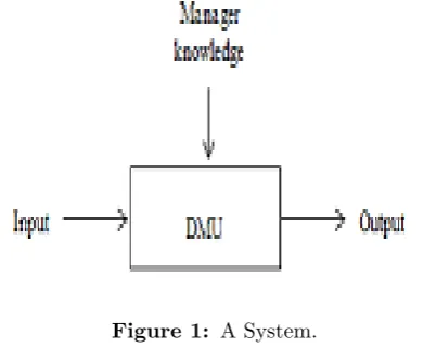
In this section some radial and non-radial mod-els are proposed that regard restricted variations. Actually, in the real world, there are occasions that the input and output factors of DMUs can-not change arbitrarily. To illustrate, a DMU is not able to reach some situations. In this study, knowledge of managers and decision mak-ers about resources, products, and DMU’s ability has a considerable effect on determining the effi-ciency of firms. The structure of this system is displayed as follows:
Figure 1: A System.
3.1 Restricted variations in radial
Models
As previous section, suppose there are n DMUs,
DM Uj(j = 1,2, ..., n), with m inputs xij, i =
1,2, ..., m and s outputs yrj, r = 1,2, ..., s.
In-efficient units in DEA should increase their out-put levels and simultaneously decrease their in-put levels according to equations (3.4) to become efficient.
∑n
j=1λjxij ≤xip, i= 1,2, ..., m,
∑n
j=1λjyrj≥yrp, r= 1,2, ..., s.
(3.4)
The conventional DEA models assume that re-ducing inputs and increasing outputs can be made arbitrarily. In real applications, however, because of limited resources, infinite variations in inputs and outputs are impossible.
Suppose the i-th input of DM Up is limited to
decrease to xip −αip ≥ 0. Similarly, the r-th
output of DM Up is limited to increase to yrp+
βrp ≥0. In other words
xip→xip−αip, i= 1,2, ..., m,
yrp→yrp+βrp, r= 1,2, ..., s
(3.5)
that αp = (α1p, α2p, ..., αmp)t and βp =
(β1p, β2p, ..., βsp)t. If ( ∑n
j=1λjxj, ∑n
j=1λjyj)be
the projection of DM Up in PPS (that is T),
clearly, we cannot expect this projection is lo-cated on the frontier.
Considering the restricted variations (i.e.(3.5)), the following constraints must be held:
∑n
j=1λjxij≥xip−αip, i= 1,2, ..., m,
∑n
j=1λjyij ≤yrp+Brp, r= 1,2, ..., s.
(3.6)
Now consider the efficiency assessment ofDM Up
in CRS environment as follows:
min θ
(θxp, yp)∈T.
By the definition of T and taking the restrictions (3.6) into consideration, we have the following lin-ear programming:
M in θ
s.t. ∑nj=1λjxij ≤θxip, i= 1,2, ..., m,
∑n
j=1λjyrj≥yrp, r= 1,2, ..., s,
∑n
j=1λjxij≥xip−αip, i= 1,2, ..., m,
∑n
j=1λjyrj≤yrp+βrp, r= 1,2, ..., s,
λj ≥0, j= 1,2, ..., n.
(3.7)
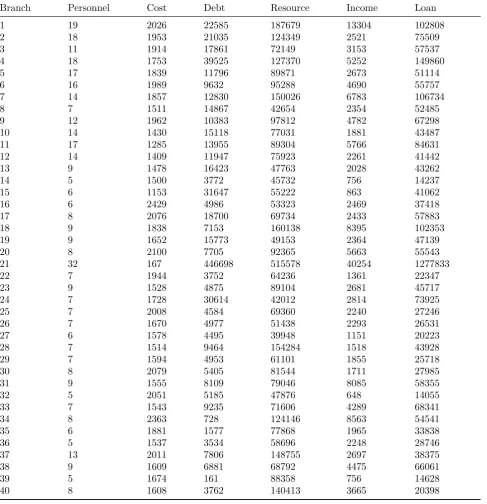
Table 1: Data for a Real Application.
Branch Personnel Cost Debt Resource Income Loan
1 19 2026 22585 187679 13304 102808
2 18 1953 21035 124349 2521 75509
3 11 1914 17861 72149 3153 57537
4 18 1753 39525 127370 5252 149860
5 17 1839 11796 89871 2673 51114
6 16 1989 9632 95288 4690 55757
7 14 1857 12830 150026 6783 106734
8 7 1511 14867 42654 2354 52485
9 12 1962 10383 97812 4782 67298
10 14 1430 15118 77031 1881 43487
11 17 1285 13955 89304 5766 84631
12 14 1409 11947 75923 2261 41442
13 9 1478 16423 47763 2028 43262
14 5 1500 3772 45732 756 14237
15 6 1153 31647 55222 863 41062
16 6 2429 4986 53323 2469 37418
17 8 2076 18700 69734 2433 57883
18 9 1838 7153 160138 8395 102353
19 9 1652 15773 49153 2364 47139
20 8 2100 7705 92365 5663 55543
21 32 167 446698 515578 40254 1277833
22 7 1944 3752 64236 1361 22347
23 9 1528 4875 89104 2681 45717
24 7 1728 30614 42012 2814 73925
25 7 2008 4584 69360 2240 27246
26 7 1670 4977 51438 2293 26531
27 6 1578 4495 39948 1151 20223
28 7 1514 9464 154284 1518 43928
29 7 1594 4953 61101 1855 25718
30 8 2079 5405 81544 1711 27985
31 9 1555 8109 79046 8085 58355
32 5 2051 5185 47876 648 14055
33 7 1543 9235 71606 4289 68341
34 8 2363 728 124146 8563 54541
35 6 1881 1577 77868 1965 33838
36 5 1537 3534 58696 2248 28746
37 13 2011 7806 148755 2697 38375
38 9 1609 6881 68792 4475 66061
39 5 1674 161 88358 756 14628
40 8 1608 3762 140413 3665 20398
e∗p=M in θ−ε[∑mi=1s−i +∑sr=1s+
r
]
s.t. ∑nj=1λjxij+s−i =θxip, i= 1, ,2, ..., m,
∑n
j=1λjyrj−s+r =yrp, r= 1, ,2, ..., s,
∑n
j=1λjxij ≥xip−αip, i= 1, ,2, ..., m,
∑n
j=1λjyrj ≤yrp+βrp, r= 1, ,2, ..., s,
λj ≥0, j= 1,2, ..., n.
(3.8)
in whichεis a very small positive constant (i.e. a non-Archimedean constant).
Definition 3.1 DM Up is said to be efficient in models (3.7) and (3.8) if and only if e∗p = 1.
Improvement in an inefficient unit is attained by the following formula:
ˆ xip ←
∑n
j=1λjxij, i= 1,2, ..., m,
ˆ yrp←
∑n
j=1λjyrj, r= 1,2, ..., s.
Table 2: The Levels of Variations for all Branches.
Branch α1 α2 α3 β1 β2 β3
1 4 405.2 6775.5 56303.7 2660.8 5140.4
2 4 390.6 6310.5 3304.7 504.2 3775.45
3 2 382.8 5358.3 21644.7 630.6 2876.85
4 5 350.6 11857.5 38211 1050.4 7493
5 4 367.8 3538.8 26934.3 534.6 2555.7
6 5 397.8 2889.6 28586.4 938 2787.85
7 4 371.4 3849 45007.8 1356.6 5336.7
8 2 302.2 4460.1 12796.2 470.8 2624.25
9 3 392.4 3114.9 29343.6 956.4 3364.9
10 4 286 4535.4 23109.3 376.2 2174.35
11 5 257 4186.5 26791.2 1153.2 4231.55
12 3 281.8 3584.1 22776.9 452.2 2072.1
13 2 295.6 4926.9 14328.9 405.6 2163.1
14 1 300 1131.6 16566.6 151.2 711.85
15 1 230.6 9494.1 15996.9 172.6 2053.1
16 1 485.8 1495.8 20920.2 493.8 1870.9
17 2 415.2 5610 48041.4 486.6 2894.15
18 3 367.6 2145.9 14745.9 1679 5117.65
19 2 330.4 4731.9 27709.5 472.8 2356.95
20 2 420 2311.5 154673.4 1132.6 2777.15
21 7 33.4 134009.4 19270.5 8050.8 63891.65
22 1 388.8 1125.6 26731.2 272.2 1117.35
23 3 305.67 1462.5 12603.6 536.2 2285.85
24 2 345.6 9184.2 20808 562.8 3696.25
25 1 401.6 1375.2 15431.4 448 1362.3
26 2 334 1493.1 11984.4 458.6 1326.55
27 1 315.6 1348.5 46285.5 230.2 1011.15
28 1 302.8 2839.2 18330.3 303.6 2196.4
29 2 318.8 1485.9 24463.2 371 1285.9
30 2 415.8 1621.5 23713.8 342.2 1399.25
31 3 311 2432.7 23713.8 1617 2917.75
32 1 410.2 1555.5 14362.8 129.6 702.75
33 2 308.6 2770.5 21481.8 857.8 3417.05
34 2 472.6 218.4 37243.8 1712.6 2727.05
35 1 376.2 473.1 23360.4 393 1691.9
36 1 307.4 1060.2 17608.8 449.6 1423.8
37 4 402.2 2341.8 44626.5 539.4 1918.75
38 2 321.8 2064.3 20367.6 895 3303.05
39 1 334.8 48.3 26507.4 151.2 731.4
40 2 321.6 1128.67 42123.9 733 1019.9
An important point to be noted is that unlike the traditional DEA models, there is no guaran-tee that the peer unit (∑nj=1λjxj,
∑n
j=1λjyj) is
efficient.
The dual formulation of the LP model (3.7)
is given by
M ax ∑sr=1(ur−µr)yrp+
∑m
i=1ρi(xip−αip)−
∑s
r=1µrβrp
s.t.∑sr=1(ur−µr)yrj−
∑m
i=1(νi−ρi)xij ≤0, j = 1,2, ..., n,
∑m
i=1νixip = 1,
ur, µr, νi, ρi≥0, ∀i,∀r.
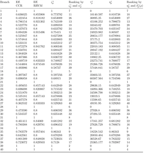
Table 3: The Results for the Real Case Example.
Branch Eff. Eff. ζp∗ Ranking by τp∗ η∗p Ranking by
CCR RRVM ζp∗ andψp∗ ηp∗andδp∗(ρ)
1 1 1 1 7 0 1 7
2 0.636025 0.855908 0.773792 11 10140.597 0.810738 10
3 0.422454 0.818182 0.653009 26 30895.25 0.653009 27
4 0.786154 0.921302 0.742109 13 45106.252 0.798673 13
5 0.522770 0.8 0.699359 18 33343.02 0.699701 20
6 0.537073 0.8 0.633792 34 35470.703 0.635167 34
7 0.894326 0.915496 0.75415 12 24923.982 0.80507 12
8 0.525947 0.8 0.627208 35 20654.177 0.678984 23
9 0.574844 0.8 0.633803 33 37175.2 0.633803 35
10 0.533131 0.8 0.645312 27 30375.754 0.645312 28
11 0.872278 0.941762 0.800346 10 22010.183 0.808505 11
12 0.550701 0.8 0.688427 21 28947.192 0.688427 21
13 0.384028 0.8 0.641628 29 22122.1 0.641628 30
14 0.467366 0.8 0.636722 30 18862.25 0.636722 31
15 0.449719 0.833333 0.740927 14 23273.741 0.760077 17
16 0.544604 0.874548 0.676026 24 25266.726 0.676026 25
17 0.493986 0.8 0.58737 39 57448.841 0.58737 39
18 1 1 1 5 0 1 6
19 0.397567 0.8 0.597256 37 35603.55 0.597256 37
20 0.696858 0.8 0.68915 20 60387.564 0.734586 19
21 1 1 1 1 0 1 1
22 0.495655 0.857143 0.642949 28 29636.15 0.642949 29
23 0.696698 0.820067 0.715532 16 16094.366 0.748255 18
24 0.551870 0.8 0.593213 38 34598.798 0.593213 38
25 0.535181 0.857143 0.678806 23 19019.5 0.678806 24
26 0.407578 0.8 0.635743 31 15598.65 0.635743 32
27 0.362532 0.833333 0.529263 40 49191.95 0.529263 40
28 1 1 1 6 0 1 5
29 0.473590 0.8 0.606592 36 27926.8 0.606592 36
30 0.534537 0.8 0.635448 32 27494.55 0.635448 33
31 1 1 1 8 0 1 8
32 0.461411 0.84069 0.681282 22 17161.257 0.681282 22
33 0.780388 0.829781 0.696452 19 27626.729 0.780674 16
34 1 1 1 3 0 1 3
35 0.783579 0.957404 0.86343 9 18228.542 0.86343 9
36 0.642561 0.8 0.670288 25 20850.404 0.670288 26
37 0.801389 0.848838 0.723024 15 36528.67 0.782222 15
38 0.723072 0.829503 0.7128 17 25365.177 0.792907 14
39 1 1 1 2 0 1 2
40 1 1 1 4 0 1 4
Theorem 3.1 The radial restricted variation model (RRVM) represented in (3.7) is feasible and bounded.
Proof. The feasibility of model (3.7) is obvious. Because θ = 1,λp = 1, λj = 0, j = 1, ..., n, j ̸=p
satisfies all constraints. Thus, it is a feasible so-lution. Furthermore, the optimal solution is not greater than one because the problem is
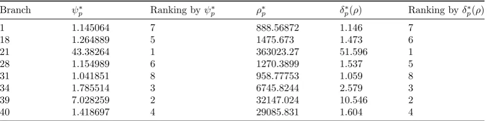
Table 4: The Results of Models (3.12), (3.15), and (3.16).
Branch ψp∗ Ranking by ψp∗ ρp∗ δ∗p(ρ) Ranking byδp∗(ρ)
1 1.145064 7 888.56872 1.146 7
18 1.264889 5 1475.673 1.473 6
21 43.38264 1 363023.27 51.596 1
28 1.154989 6 1270.3899 1.537 5
31 1.041851 8 958.77753 1.059 8
34 1.785514 3 6745.8244 2.579 3
39 7.028259 2 32147.024 10.546 2
40 1.418697 4 29085.831 1.604 4
and it guarantees that model (3.7) (RRVM) is bounded, and this completes the proof.
Theorem 3.2 Let DM Upˆ be the projection of
DM Up in model (3.7). Then DM Upˆ dominates
DM Up.
Proof. Clearly, the first and second constraints of model (3.7) imply that
ˆ
xip=∑nj=1λjxij =
θxip−s−i ≤xip, i= 1,2, ..., m,
ˆ
yrp= ∑n
j=1λjyrj =
yrp+s+r ≥yrp, r= 1,2, ..., s.
and strict inequality is held at least for one com-ponent, that is, θ < 1 andθxip < xip; therefore,
ˆ
xip< xip . This completes the proof.
3.2 Restricted Variations in
Non-Radial Models
In this subsection, two non-radial restricted DEA approaches are provided. The first approach is an extension of SBM model proposed by Tone [10] as follows:
M in ζp∗= (1−m1 ∑mi=1 s
− ip xip)/(1 +
1
s
∑s r=1
s+ rp yrp)
s.t. ∑nj=1λjxij+s−ip=xip, i= 1,2, ..., m,
∑n
j=1λjyrj−s +
rp=yrp, r= 1,2, ..., s,
∑n
j=1λjxij≥xip−αip, i= 1,2, ..., m,
∑n
j=1λjyrj≤yrp+βrp, r= 1,2, ..., s,
λj ≥0, j= 1,2, ..., n.
(3.11)
s−ip and s+rp called slacks show the excesses of in-puts and shortfalls of outin-puts forDM Up,
respec-tively. The third and fourth constraints indicate the amount of variations in inputs and outputs, respectively.
Definition 3.2 model (3.11) is efficient if and only if ζp∗ = 1. It means all inputs and outputs slacks are equal to zero.
Furthermore, for ranking the efficient DMUs and discriminating the efficient DMUs, the following model is proposed. Model (3.12) is an extension of slacks-based super-efficiency model proposed by Tone [11].
M in ψ∗p =
(1 +m1 ∑mi=1 t
− ip xip)/(1−
1
s
∑s r=1
t+rp yrp)
s.t. ∑nj=1,j̸=pλjxij ≤xip+t−ip, i= 1,2, ..., m,
∑n
j=1,j̸=pλjyrj≥yrp−t+rp, r= 1,2, ..., s,
∑n
j=1,j̸=pλjxij≥xip−αip, i= 1,2, ..., m,
∑n
j=1,j̸=pλjyrj≤yrp+βrp, r= 1,2, ..., s,
λj≥0, t−ip≥0, t+rp≥0, j= 1,2, ..., n, j ̸=p
i= 1,2, ..., m, r= 1,2, ..., s.
(3.12)
where ψp∗ ≥ 1. Furthermore, models (3.11) and (3.12) can be transformed into the linear programming problems by using Charnes and Cooper transformation [3].
varia-tion levels like the following exist:
M ax τp∗=∑mi=1s−ip+∑sr=1s+
rp
s.t. ∑nj=1λjxij+s−ip =xip, i= 1,2, ..., m,
∑n
j=1λjyrj−s+rp=yrp, r= 1,2, ..., s,
∑n
j=1λjxij ≥xip−αip, i= 1,2, ..., m,
∑n
j=1λjyrj≤yrp+βrp, r= 1,2, ..., s,
λj≥0, j= 1,2, ..., n.
(3.13)
In the above model,DM Upis efficient if and only
if all slacks are zero. Furthermore, the follow-ing formula is used for estimatfollow-ing the efficiency score:
ηp∗= (1− 1 m
m
∑
i=1 s−∗ip
xip
)/(1 + 1 s
s
∑
r=1 s+rp∗
yrp
) (3.14)
in which s−∗ip and s+rp∗ are obtained from model (3.13).
In this case, for distinguishing between efficient DMUs, the following model is presented:
M in ρ∗p=∑mi=1t−ip+∑sr=1t+
rp
s.t. ∑nj=1,j̸=pλjxij≤xip+t−ip, i= 1,2, ..., m,
∑n
j=1,j̸=pλjyrj≥yrp−t+rp, r= 1,2, ..., s,
∑n
j=1,j̸=pλjxij ≥xip−αip, i= 1,2, ..., m,
∑n
j=1,j̸=pλjyrj≤yrp+βrp, r= 1,2, ..., s,
λj≥0, t−ip≥0, t
+
rp≥0, j= 1,2, ..., n, j ̸=p
i= 1,2, ..., m, r= 1,2, ..., s.
(3.15)
Then,
δ∗p(ρ) =
(1
m
∑m
i=1
(xip+t−∗ip(ρ)) xip )/(
1
s
∑s r=1
(yrp−t+rp∗(ρ)) yrp )
(3.16)
is determined thatt−∗ip (ρ) andt+∗
rp(ρ) are attained
from model (3.15). δp∗(ρ) is used as the super-efficiency score which δp∗(ρ) ≥ 1. t−ip and t+rp in models (3.12) and (3.15) denote the increase of inputs and the decrease of outputs for the efficient
DM Up while the frontier has been made by the
remaining DMUs.
Theorem 3.3 Models (3.12) and (3.15) are fea-sible.
Proof. As Tone [11] and Du et al. [7], we also assume
˜
t−ip = max{xip, ∑n
j=1,j̸=p˜λjxij} − xip ≥ 0, i =
1, ..., m, ˜
t+rp = yrp −min{yrp, ∑n
j=1,j̸=pλ˜jyrj} ≥ 0, r =
1, ..., s. Therefore,
xip + ˜t−ip = max{xip, ∑n
j=1,j̸=pλ˜jxij} ≥ ∑n
j=1,j̸=p˜λjxij and
yrp − ˜t+rp = min{yrp, ∑n
j=1,j̸=p˜λjyrj} ≤ ∑n
j=1,j̸=p˜λjyrj.
Furthermore, ˜λjj = 1, ..., n, j ̸= p is
con-sidered as a non-negative set such that
∑n
j=1,j̸=p˜λjxij ≥xip−αip, i= 1,2, ..., m, ∑n
j=1,j̸=p˜λjyrj ≤yrp+βrp, r= 1,2, ..., s.
Thus,
˜
t−ip, i = 1, ..., m, ˜t+rp, r = 1, ..., s, and ˜λj
j= 1, ..., n, j̸=p
is a feasible solution for models (3.12) and (3.15).
4
A Real Application
In this section we examine the validity of the re-stricted DEA models by using a real data set. We apply the approaches to a data set consisting 40 branches of a commercial bank in one region in Iran. We have used six variables from the data set as inputs and outputs. Each branch uses three in-puts and three outin-puts. Inin-puts include number of staff, operational costs (excluding staff costs) and overdue debts; outputs are deposits (resources), amount of income and amount of loans. The cho-sen input and output measures that are used in the application are summarized in Table 1 (All monetary variables are stated in ten million of Iranian current Rials). Table2contains listing of the levels of variations in inputs and outputs of each branch j forj = 1, ...,40 that are predicted by the board of management. The defined limited values are associated with management’s points of view and unit location. In Table2, columns 2, 3, and 4 show the variations levels in inputs(αi)
while the variations levels in outputs (βr)are
21, 28, 31, 34, 39, and 40 are obtained. This is confirmed by our proposed models. The results are listed in Table3. As columns 2 and 3 of the ta-ble show, efficiency measures of inefficient units in model (3.7) (RRVM) are greater than that of the CCR-model. This means that the target unit ob-tained from model (3.7) is closer than the target obtained from the CCR model for the unit under evaluation. Furthermore, one can contrast the results of SBM and additive models with models (3.11) and (3.14), respectively. It is found that the efficiency measures of non-radial restricted variation models, models (3.11) and (3.14), will be greater than the SBM and additive models. This is the advantage of our models in the sense that we took the ability of the units into consid-eration. Columns 4, 6, and 7 in Table3show the results of models (3.11), (3.13) and (3.14), respec-tively. Also, the results of ranking branches by using the restricted variation SBM approach and the restricted variation additive approach can be seen in columns 5 and 8 of Table 3, respectively. In both approaches, branch 21 has been distin-guished as the most efficient while branch 27 has been determined as the least efficient. Neverthe-less, there are some differences between rankings of the two methods. Table4represents the results of models (3.12), (3.15) and (3.16). To illustrate, the results of ranking the efficient branches can be found in Table4. As can be seen, except ranks of 18 and 28 branches, ranks of other branches are the same when model (3.12), models (3.15) and (3.16) are calculated.
5
Concluding Remarks
In the real world, there are application cases in which inefficient units cannot reduce their inputs and increase their outputs arbitrarily to become efficient. In these cases, the target units for these operational units do not necessarily belong to the efficient frontier. The current paper has proposed modified DEA models in such a restricted en-vironment. Indeed, it has been imported these limitations in some DEA models and proposed new models, radial and non-radial models, in or-der to assess the relative efficiency of these ap-plication cases. In models proposed, inefficient units are not necessarily projected onto the effi-cient frontier, but the projections dominate inef-ficient units. Moreover, some non-radial ranking
approaches have been extended for distinguishing the efficient DMUs where restricted variations ex-ist. An application area investigated involved 40 branches of a commercial bank. It seems incor-porating unbalanced data with missing values in the proposed models is an interesting subject for future research.
Acknowledgement
Financial support by Lahijan Branch, Islamic Azad University Grant No. 1235, 17-20-5/3507 is gratefully.
References
[1] P. Andersen, N. C. Petersen, A procedure for ranking efficient units in data envel-opment analysis, Management Science 39 (1993) 1261-1264.
[2] R. D. Banker, A. Charnes, W. W. Cooper,
Some models for estimating technical and scale inefficiencies in data envelopment analysis, Management Science 30 (1984) 1078-1092.
[3] A Charnes, W. W. Cooper, Programming with linear fractional functionals, Naval Re-search Logistics Quarterly 9 (1962) 181-186. [4] A. Charnes, W. W. Cooper, L. Seiford, J. Stutz, A multiplicative model for efficiency analysis, Socio-Economic Planning Sciences 16 (1982) 223-224.
[5] A. Charnes, W. W. Cooper, E. Rhodes,
Measuring the efficiency of decision making units, European Journal of Operational Re-search 2 (1978) 429-44.
[6] J. Doyle, R. Green, Efficiency and cross-efficiency in DEA: Derivations, meanings and uses, Journal of the Operational Re-search Society (1994) 567-578.
[7] J. Du, L. Liang, J. Zhu, A slacks-based mea-sure of super-efficiency in data envelopment analysis: a comment, European Journal of Operational Research 204 (2010) 694-697. [8] S. Kordrostami, A. Amirteimoori, M. J. S.
nature, International Journal of Biomathe-matics 8 (2015) 1550034.9
[9] L.M. Seiford, J. Zhu, Infeasibility of super-efficiency data envelopment analysis models, Infor. 37 (1999) 174-187.
[10] K. Tone, A slacks-based measure of effi-ciency in data envelopment analysis, Euro-pean Journal of Operational Research 130 (2001) 498-509.
[11] K. Tone, A slacks-based measure of super-efficiency in data envelopment analysis, Eu-ropean Journal of Operational Research 143 (2002) 32-41.
Sohrab Kordrostami is a full pro-fessor in applied mathematics (op-erations research field) department in Islamic Azad University, Lahi-jan branch. He completed his Ph.D. degree in Islamic Azad Uni-versity of Tehran, Iran. His re-search interests include performance management with special emphasis on the quantitative meth-ods of performance measurement, and especially those based on the broad set of methods known as Data Envelopment Analysis, (DEA). Kor-drostami’s papers have appeared in a wide se-ries of journals such as Applied mathematics and computation, Journal of the operations research society of Japan, Journal of Applied mathemat-ics, International journal of advanced manufac-turing technology, International journal of pro-duction economics, Optimization, International Journal of Mathematics in Operational research, Journal global optimization, etc.
Alireza Amirteimoori is a full pro-fessor in applied mathematics op-erations research group in Islamic Azad University in Iran. He com-pleted his Ph. D degree in Is-lamic Azad University in Tehran, Iran. His research interests lie in the broad area of performance management with special emphasis on the quantitative methods of performance measurement, and especially those based on the broad set of methods known as Data
Envelopment Analysis, (DEA). Amirteimoori’s papers appear in journals such as Applied math-ematics and computation, Journal of the opera-tions research society of Japan, Journal of Ap-plied mathematics, RAIRO-Operations research, International journal of advanced manufacturing technology, International Journal of Production Economics, Optimization, Expert Systems with Applications, Central European Journal of Oper-ational Research, InternOper-ational Journal of Math-ematics in Operational Research, Decision Sup-port Systems, Journal of Global Optimization and etc.