Vol. 8, No. 3, 2016 Article ID IJIM-00784, 10 pages Research Article
Numerical Solution of Fractional Control System by Haar-wavelet
Operational Matrix Method
M. Mashoof∗, A. H. Refahi Sheikhani †‡
Received Date: 2015-11-09 Revised Date: 2016-01-05 Accepted Date: 2016-02-11
————————————————————————————————–
Abstract
In recent years, there has been greater attempt to find numerical solutions of differential equations using wavelet’s methods. The following method is based on vector forms of Haar-wavelet functions. In this paper, we will introduce one dimensional Haar-wavelet functions and the Haar-wavelet opera-tional matrices of the fracopera-tional order integration. Also the Haar-wavelet operaopera-tional matrices of the fractional order differentiation are obtained. Then we propose the Haar-wavelet operational matrix method to achieve the Haar-wavelet time response output solution of fractional order linear systems where a fractional derivative is defined in the Caputo sense. Using collocation points, we have a Sylvester equation which can be solve by Block Krylov subspace methods. So we have analyzed the errors. The method has been tested by a numerical example. Since wavelet representations of a vector function can be more accurate and take less computer time, they are often more useful.
Keywords: Fractional control system; Haar wavelet; Sylvester equation.
—————————————————————————————————–
1
Introduction
F
rized from integer order ones, which achievedactional differential equations have general-by replacing integer order derivatives general-by frac-tional ones. In recent years, studies on appli-cation of the FDE in science has been attract-ing more attention [5, 22, 8, 27] and the reader may refer to [22, 8] for the theory and applica-tions of fractional calculus. For instance, Bagley and Torvik formulated the motion of a rigid plate immersing in a Newtonian fluid [22, 8, 20]. It shows that the use of fractional derivatives for the mathematical modelling of viscoelastic materials is quite natulral [22]. It should be mentioned that ∗Department of Mathematics, Lahijan Branch, Islamic Azad University, Lahijan, Iran.†Corresponding author. ah [email protected]
‡Department of Mathematics, Lahijan Branch, Islamic Azad University, Lahijan, Iran.
the main reasons for the theoretical development are mainly the wide use of polymers in various fields of engineering [22]. Also in 1991, S. West-erlund suggested using fractional derivatives for the description of propagation of plane electro-magnetic waves in an isotropic and homogeneous, lossy dielectric and in the paper on electrochem-ically polarizable media, published in 1993[22]. Caputo suggested the fractional-order version of the relationship between electric field and electric flux density [22].
Recently, fractional derivatives have been used to new applications in neural networks and control system [25].
A typical n-term linear non-homogeneous frac-tional order differential equation (FDE) in time
domain can be described as the following form,
an(Dαn
t y(t)) +· · ·+a1(Dαt1y(t))+
+a0(Dαt0y(t)) =u(t).
(1.1)
A fractional-order system described by n-term fractional differential Eq. (1.1) can be rewrit-ten to the state-space representation in the form [11,30]:
aDβtx(t) =Ax(t) +Bu(t)
y(t) =Cx(t) . (1.2)
For this reason the behavior of output in system 1.2are useful.
Wavelets are mathematical tools that cut up data, functions or operators into different frequency components and then study each component with a resolution matching its scale. Much of the work on Haar functions was per-formed in the 1930s. In 1909, Haar discovered the simplest function that is called as Haar wavelet. The integral of Haar family called Haar operational matrix was derived by Chen and Hsiao [7] in 1997. Recently, Operational matrix method has became a very useful technique for solving fractional differential equations [28,23,6] and optimal control system [17].
In this paper, we will present Haar-wavelet time response of the fractional order system of the form
aDαtx(t) =Ax(t) +Bu(t) y(t) =Cx(t) +Du(t), 0≤t≤η, x(0) =( λ1, λ2,· · ·, λn
)T ,
(1.3)
with 0< α≤1, whereA,B,C andDaren×n, n×m,p×nandp×m matrices respectively and u(t) is an m-vector function.The rest of the paper has organized as follows: in Section 2 we recall some necessary definitions and theorems. The Function approximations and operational matri-ces is presented in Section 3. In Section 4, we express the method of the solution and the error analysis are study in Section5. Section6contain one numerical example and Finally, the main con-clusions are drawn in Section7.
2
Preliminaries
In this Section, we present some basic definitions and properties of fractional calculus [22,9,26].
Definition 2.1 A real function f(x), x ≥ 0 is said to be in space Cµ, µ∈R if there exists a real number p(> µ), such that f(x) =xpf1(x) where
f1(x) ∈ [0,∞) , and it is said to be in the space
Cµm iff fm∈Cµ, m∈N.
Definition 2.2 The Riemann-Liouville frac-tional derivative of order α with respect to the variable x and with the starting point at x=ais
aDtαf(x)
= Γ(−α+1m+1)dxdmm+1+1
∫x
a(x−τ)m−αf(τ)dτ, (2.1) for 0≤ m≤α < m+ 1and
aDαtf(x) = dm+1 dxm+1f(x)
for α=m+ 1∈N.
Definition 2.3 The Riemann-Liouville frac-tional integral of order α is
aDt−αf(x) = 1 Γ(α)
∫ x
a
(x−τ)α−1f(τ)dτ, α >0. (2.2)
Definition 2.4 The fractional derivative off(x) by means of Caputo sense is defined as
Dαtf(x)
= Γ(n1−α)∫0x(x−τ)n−α−1f(n)(τ)dτ,
(2.3)
where n−1< α≤n, n∈N, x >0, f ∈C−n1.
For the Caputo’s derivative we haveDα
tC= 0,C is a constant.
Definition 2.5 (Fractional Derivative of a Vec-tor) If X(x) = (X1(x)· · ·Xn(x))T is a vector
function, we define
DxαX(x) =( DαxX1(x),· · ·, DαxXn(x) )T
. (2.4)
Definition 2.6 The m-set of block-pulse func-tions is defined as:
bi(t) = {
1 ; ηim ≤t≤ η(im+1)
0 ; otherwise (2.5)
for i= 0,1,2,· · ·, m−1.
Definition 2.7 (The Haar Wavelet Function) Let [0, η) be an interval, we define h0(t) and
h1(t) on[0, η) as follows
h0(t) = √1η
{
1 ; 0≤t < η, 0 ; otherwise,
h1(t) = √1η
1 ; 0≤t < η2, −1 ; η2 ≤t <1,
0 ; otherwise,
and for i= 2j +k , j ⩾0 , 0 ≤k≤2j −1, we define
hi(t) = 2
j
2
√ηh1(2jt−k).
The best way to understand wavelets is through a multi-resolution analysis. Given a function f ∈ L2(R) a multi-resolution analysis (MRA)
of L2(R) produces a sequence of subspaces
Vj, Vj+1, · · ·such that the projections off onto
these spaces give finer and finer approximations of the function f asj→ ∞.
Definition 2.8 (Multi-resolution Analy-sis(MRA)) A multi-resolution analysis of L2(R) is defined as a sequence of closed sub-spaces Vj ⊂ L2(R), j ∈ Z with the following properties
i) · · · ⊂V−1 ⊂V0 ⊂V1· · ·.
ii) The spaces Vj satisfy ∪j∈ZVj is dense in L2(R) and ∩j∈ZVj = 0.
iii) If f(x) ∈ V0,f(2jx) ∈ Vj, i.e. the spaces Vj are scaled versions of the central space V0.
iv) If f(x) ∈ V0,f(2jx−k) ∈ Vj, i.e. all the Vj are invariant under translation.
v) There exists ϕ∈V0 such that ϕ(x−k);k∈Z
is a Riesz basis inV0.
The space Vj is used to approximate general functions by defining appropriate projection of these functions onto these spaces. Since the union of all the Vj is dense in L2(R), so it guarantees that any function inL2(R) can be ap-proximated arbitrarily close by such projections. As an example the space Vj can be defined like
Vj =Wj−1⊕Vj−1 =Wj−1⊕Wj−2⊕Vj−2
=· · ·=⊕ji=0−1Wi⊕V0
then the scaling function h0(x) generates
an MRA for the sequence of spaces {Vj, j ∈ Z}
by translation and dilation as defined in def-inition 2.8. For each j the space Wj serves as the orthogonal complement of Vj in Vj+1. The
space Wj include all the functions in Vj+1 that
are orthogonal to all those in Vj under some chosen inner product. The set of functions which form basis for the space Wj are called wavelets [13,21].
The following theorem gives several equivalent statements which permit us to check if an orthonormal system is also a basis:
Theorem 2.1 Given an orthonormal system x1, x2,· · · in E, the following are equivalent:
i) The set of vectors x1, x2,· · · is an orthonormal
basis for E.
ii) If < xi, y >= 0 for i = 1,2,· · ·, then y = 0, where < x, y > is the inner product of x and y. iii)span(xi)is dense inE, that is, every vector in E is a limit of a sequence of vectors inspan(xi). iv) For every y in E,
||y||2=∑i|< xi, y >|2, which is called Parsevals equality. v) For every y1 and y2 in E,
< y1, y2>=
∑
i< xi, y1 >∗< xi, y2 >,
which is often called thegeneralized Parsevals equality.
Proof. see [12].
Lemma 2.1 Every characteristic function of the formχ[0,k/2n)(t) is a finite linear combination
of the hi(t).
Proof. We will induct on n. Let Pn be the statement that for all integers k with 0 ≤ k ≤ 2n − 1 the characteristic function χ[0,k
2nη)(t) is finite linear combination of the
hi. P0 is true, since χ[0,η)(t) =
√
(η)h0(t).
Assume that Pn is true. We use this to show that χ[0, k
2n+1η)
is a finite linear combination of hi. We first do the case when k ≤ 2n−1. Since Pn is true we haveχ[0,k
2nη)(t) =
∑
iaihi(t), butχ[0, k
2n+1η)(t) =χ[0,
k
2nη)(2t), thus we can write
χ[0, k
2n+1η)
(t) = { ∑
iaihi(t) ;t≤ η
2
0 ;t > η2 , and therefore Pn+1 is true. Now we need
to take care of the case when k > 2n−1. We first observe that if k >2n−1 then
χ[0, k
2n+1η)
=χ[0,1 2η)+χ[
1 2η,
k
2n+1η)
We already know that χ[0,1
2η) is a finite
lin-ear combination of the hi, so we only need to show thatχ[1
2η,
k
2n+1η) is too. Observe that
χ[1 2η,
k
2n+1η)
(t) =χ[0,k−2n
2n η)
(2t−η),
applying the assumption that Pn is true for the above equality and the proof can be completed.
Theorem 2.2 Any function y(t) ∈ L2[0, η) can be decomposed as
y(t) =
∞
∑
i=0
cihi(t), (2.6)
where the coefficients ci are determined by
ci = 2j∫0ηy(t)hi(t)dt, i= 2j+k, j⩾0, 0≤k≤ 2j−1.
Proof. Let f ∈ L2[0, η) such that ∫η
0 f(t)hi(t)dt = 0 for i = 0,1,· · ·.
there-fore ∫ k
2nη
0 f(t)dt =
∫η
0 χ[0,2knη)(t)f(t)dt =
∫η
0(
∑
iaihi(t))f(t)dt= 0.
The set of all numbers of the form 2knη are
dense in R and for evry x ∈ R there is an increasing sequence xi such that xi → x. This shows that ∫0xf(t)dt = 0 for all x ∈ [0, η) and therefore f = 0, so theorem 2.9 shows that hi, i= 0,1,· · · is a basis forL2[0, η)■
Theorem 2.3 Assume that y(t) ∈ L2(R) with the bounded first derivative on (0,1)and ym(t) = ∑2m+1
i=0 cihi(t), then ||y(t)−ym(t)||2
=∑∞i=m∑∞j=mcicj∫−∞∞ hi(t)hj(t)dt
≤ k
7c22−
3
2m ,
(2.7)
where c=∫01|th2(t)|dt andk is a constant and
||g(t)||= (∫−∞∞ g2(t)dt) 12.
Proof. The error at Jth level may be defined as |eJ(t)|= |y(t)−yJ(t)|= ∑∞i=2J+1+1cihi(t) where
yJ(t) = ∑2J+1
i=1 cihi(t). Thus we have
||eJ(t)||2
= ∫ ∞
−∞( ∞
∑
i=2J+1+1
cihi(t),
∞
∑
l=2J+1+1
clhl(t))dt
=
∞
∑
i=2J+1+1 ∞
∑
l=2J+1+1
cicl ∫ ∞
−∞hi(t)hl(t)dt,
this shows that
||eJ(t)||2≤
∞
∑
i=2J+1+1
|ci|2. (2.8)
But |ci|≤ c2−32imax(y′(η)) where c =
∫1
0|th2(t)|dt and η∈(k2−
j,(k+ 1)2−j)[14,16]. Thus
||eJ(t)||2≤∑∞i=2J+1+1kc22−3i,
where |y′(t)|≤ k for all t ∈ (0,1) and k is a positive constant. From the last relation we have
||eJ(t)||2≤kc2 172−3m, or
||eJ(t)||≤ √
k
7c2−
3 2m ■
In our survey, the fractional derivatives and fractional integrals have considered in the Ca-puto and Riemann-Liouville sense, respectively. For more details see [22,3]. Let us consider the fractional differential equation
Dtαx(t) =Ax(t) +q(t), (2.9)
with 0 < α < 1, an N ×N matrix A, a given functionq: [0, h]→CN and an unknown solution x : [0, h] → CN. Two following theorems shows the form of the general solution of (2.9) where Eα(t) is the Mittag-Leffler function.
Definition 2.9 The Mittag-Leffler function with parameter α is given by
Eα(z) =
∞
∑
k=0
zk
Γ(αk+ 1), ℜ(α)>0, z∈C.
Theorem 2.4 Let λ1,· · ·, λN, be the eigenval-ues of A and u(1),· · ·, u(N) be the corresponding eigenvectors. Then, the general solution of the the homogeneous differential equation Dαtx(t) = Ax(t), has the form
x(t) = N ∑
l=1
clu(l)Eα(λlxα), (2.10)
with certain constants cl ∈ C. The unique so-lution of this differential equation subject to the initial conditionx(0) =x0 is characterized by the
linear system
x0= (u(1),· · ·, u(N))(c1,· · ·, cN)T. (2.11)
Proof. see [10].
For the inhomogeneous boundary value problem we can state the following result.
Theorem 2.5 The general solution of the boundary value problem (2.9) has the form x = xhom + xinhom where xhom is the general solu-tion of the associated homogeneous problem and xinhom is a particular solution of the inhomoge-neous problem.
Proof. see [10].
3
Function approximations and
operational matrices
The series expansion of y(t) in (2.6) contains an infinite terms. If y(t) is piecewise constant by itself, or may be approximated as piecewise constant during each subinterval, then y(t) will be terminate at finite terms, that is
y(t)≃ m∑−1
i=0
cihi(t) =CmTHm(t), (3.12)
where T indicates transposition and Cm =
(
c0 c1 · · · cm−1
)T
is the Haar coefficient vector of y(t) and Hm(t) = (
h0(t) h1(t) · · · hm−1(t)
)T
and m= 2j . At collocation points ti = 22i+1m , i = 0,1,· · ·, m − 1, one can define m × m Haar matrix as
Hm×m
=( Hm(t0) Hm(t1) · · · Hm(tm−1)
) .
Since Hm×m is singular [9, 26], the Haar coefficients ci, i = 0,1,2,· · ·, m−1 can be also be determined by matrix inversion as follows
CmT =ymHm−1×m,
ym =( y(t0) y(t1) · · · y(tm−1)
) .
(3.13)
The integration of Haar function vectorHm(t) is given by
∫ t
0
Hm(s)ds≃Pm×mHm(t), (3.14)
where Pm×m is the Haar wavelet operational matrix of integration [26] and is given by
Pm×m= 21m (
2mPm
2×
m
2 −H
m
2×
m
2
H−m1
2×
m
2 0
) .
Also the Haar wavelets can be expand into m-set of block-pulse functions as
Hm(t) =Hm×mBm(t) (3.15)
where the block-pulse function vec-tor Bm(t) is defined as Bm(t) = (
b1(t) b2(t) · · · bm−1(t)
)T
. Fractional integration of the block-pulse function vector is given as
(IαBm)(t) =FαBm(t), (3.16) where Fα is the block-pulse operational matrix of the fractional order integration [18]. The Haar wavelet operational matrix of fractional order in-tegration can be derive as following [19],
(IαHm)(t) =Pmα×mHm(t), (3.17)
wherePα
m×mis the Haar wavelet operational ma-trix of fractional order integration and can be ob-tained by substituting (3.15) and (3.16) in (3.17) as
Pmα×m=Hm×mFαHm−1×m. (3.18)
4
Method of solution
In this Section we consider the fractional order system . From1.3 we find that
Dαxi(t) =Aix(t) +Biu(t). (4.19)
Also from (3.12) we can approximate each xi(t) by
thus we can set
x(t) =CxHm(t), (4.21)
whereCx= (
C1T,m, C2T,m,· · ·, Cn,mT )T ,
similarly u(t) = CuHm(t) where Cu can de-rived by (3.13), now we have
(IαDαxi)(t) =Iα(Aix+Biu)(t)
⇒
xi(t) =AiCx(IαHm)(t)+
+BiCu(IαHm)(t) +xi(0),
(4.22)
using (3.16), (3.17) and (3.18) in (4.22) we have
xi(t)
= (AiCx+BiCu)Hm×mFαHm−1×mHm(t)+
+xi(0),
(4.23) or in matrix form
x(t)
= (ACx+BCu)Hm×mFαHm−1×mHm(t)+
+x(0).
(4.24) Now by (4.21) and (4.24) we find that
CxHm(t)
= (ACx+BCu)Hm×mFαHm−1×mHm(t)+
+x(0),
(4.25) dispersing (4.25) by the collocation points ti we can obtain
CxHm×m
= (ACx+BCu)Hm×mFαHm−1×mHm×m
+X0,
where X0 =
(
x(0) x(0) · · · x(0) ), thus we have
CxHm×m(Hm×mFα)−1−ACx
=BCu+X0(Hm×mFα)−1,
(4.26)
which is a Sylvester equation. This equation can be solve by Block Krylov subspace methods [24]. From above discussion we can response output of system as
y(t) =Cx(t)≃(CCx+DCu)Hm(t). (4.27)
5
The error analysis
Theorem 5.1 Assume that theorem 2.8 holds for xi(t);i= 1,2,· · ·, n, then we have
||CxHm(t)−x(t)||2≤nk 7c
22−32m. (5.28)
Proof: The error may be defined as
||v(t)||= ( ∫ ∞
−∞v
T(t)v(t))12
(v(t) is a column vector). So ∥CxHm(t)−x(t)∥2
=∥( C1T,mHm(t) · · · Cn,mT Hm(t) )T
− −( ∑∞i=0ci,1hi(t) · · ·
∑∞
i=0ci,nhi(t)
)T ∥2
=∥
∞
∑
i=2m (
ci,1hi(t) · · · ci,nhi(t)
)T ∥2
= ∫ ∞
−∞( ∞
∑
i=2m
ci,1hi(t)
∞
∑
j=2m
cj,1hj(t) +· · ·+
+
∞
∑
i=2m
ci,nhi(t)
∞
∑
j=2m
cj,nhj(t))
= n ∑
l=1
∞
∑
i=2m
∞
∑
j=2m ci,lcj,l
∫ ∞
−∞hi(t)hj(t)
sinceh,isare orthonormal we can indicate
∥CxHm(t)−x(t)∥2= n ∑
l=1
∞
∑
i=2m c2i,l,
and since theorem2.5holds for eachxi(t) we can write
n ∑
l=1
∞
∑
i=2m c2i,l≤
n ∑
l=1
klc2 1 72
−3J,
so
∥CxHm(t)−x(t)∥2≤ (k1+· · ·+kn) 7 c
22−3J.
■
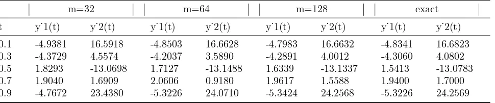
Table 1: Haar wavelet numerical solution of example6.1
m=32 m=64 m=128 exact
t y˙1(t) y˙2(t) y˙1(t) y˙2(t) y˙1(t) y˙2(t) y˙1(t) y˙2(t)
0.1 -4.9381 16.5918 -4.8503 16.6628 -4.7983 16.6632 -4.8341 16.6823 0.3 -4.3729 4.5574 -4.2037 3.5890 -4.2891 4.0012 -4.3060 4.0802 0.5 1.8293 -13.0698 1.7127 -13.1488 1.6339 -13.1337 1.5413 -13.0783
0.7 1.9040 1.6909 2.0606 0.9180 1.9617 1.5588 1.9400 1.7000
0.9 -4.7672 23.4380 -5.3226 24.0710 -5.3424 24.2568 -5.3226 24.2569
6
Examples
To demonstrate the efficiency and the practi-cability of the proposed method based on Haar wavelet operational matrix method, we consider the following example. In order to show the effi-ciency of method for solving system1.3, we apply it to solve different types of fractional linear sys-tems whose exact solutions are known. We use ∥.∥2 to compare exact and numerical solution.
Example 6.1 In this example we consider a fractional system with three equations,
Dαtx(t) =
−21 01 −09 3 6 1
x(t)
y= (
1 0 −1 −1 2 3
) x(t),
(6.29)
x(0) = −53
0
,0 ≤ t ≤ 1,0 < α ≤ 1. The
general solution of (6.29) according to theorem 2.13, is given by
x(t) =c1u1E(λ1tα) +c2u2E(λ2tα)+
+c3u3E(λ3tα),
y= (
1 0 −1 −1 2 3
) x(t),
(6.30)
where c1, c2, c3 are constants and λ1, λ2, λ3 are
eigenvalues and u1, u2, u3 are corresponding
eigenvectors of A. For α = 0.975 and m = 8 we have
Cx=
( −2.8107 −2.4681 · · · −1.1778
4.1749 1.5822 · · · 5.1485 1.2002 2.6363 · · · 2.5816
) .
Thus from (4.27) we have (
y1(t)
y2(t)
)
≃CCxH8(t).
a)
0 0.125 0.25 0.375 0.5 0.625 0.75 0.875 −15
−10 −5 0 5 10 15 20 25
t m=32
CC
x
H3
2(t)
b)
0 0.125 0.25 0.375 0.5 0.625 0.75 0.875 −15
−10 −5 0 5 10 15 20 25
t m=128
CC
x
H128
(t)
Figure 1: Output time response of example 6.1 by Haar representation for m=32, 128.
nu-a)
0 0.2 0.4 0.6 0.8 1 0
0.5 1 1.5 2 2.5 3
t
|exact y
1
(t)−numerical y
1
(t)|
m=8 m=32 m=64 m=128
b)
0 0.2 0.4 0.6 0.8 1 0
1 2 3 4 5 6 7 8 9
|exact y
2
(t)−numerical y
2
(t)|
t
m=8 m=32 m=64 m=128
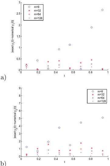
Figure 2: Absolute errors of y1(t) andy2(t) at t = 1
16, 3 16, ...,
15
16 form= 8,32,64,128.
merical solutions for different values of m. Also Fig. 2 shows the absolute errors for y1(t) and
y2(t) respectively at the collocation points ti for
m = 8,32,64,128. From Table 1, we see that we can achieve a good approximation for output with the exact solution by usingm= 64,128. The Haar domain solution along with the actual solu-tion are shown in Fig. 1.a, 1.b for m = 32,128 respectively. Table 1 shows the numerical solu-tions for different values ofm. Also Fig. 2 shows the absolute errors fory1(t)andy2(t)respectively
at the collocation points ti for m= 8,32,64,128. From Table 1, we see that we can achieve a good approximation for output with the exact solution by usingm= 64,128.
7
Conclusion
In this paper,we introduced Haar-wavelet oper-ational matrix method to fractional control sys-tem. We translated the control system with ini-tial condition into a Sylvester equation which can be solve by Block Krylov subspace meth-ods. From Section 5 we found that the error bound is inversely proportional to m. This en-sures the convergence of the Haar wavelet
ap-proximation when m is increased. An example presented in Section 6 and the results obtained are compared with exact solutions. Moreover if we use distributed order fractional derivative in-stead of fractional derivative, then what will be the form of operational matrix represented in Sec-tion 3?
References
[1] H. Aminikhah, A. Refahi Sheikhani and H. Rezazadeh, Stability Analysis of Distributed Order Fractional Chen System, The Sci. World J. (2013), http://dx.doi.org/10. 1155/2013/645080/.
[2] H. Aminikhah, A. Refahi Sheikhani and H. Rezazadeh, Stability analysis of linear dis-tributed order system with multiple time de-lays, U. P. B. Sci. Bull. 77 (2015) 207218.
[3] A. Ansari and A. Refahi Sheikhani, New identities for the Wright and the Mittag-Leffler functions using the Laplace trans-form, Asian-European Journal of Math-ematics 7 (2014) 145-150.
[4] A. Ansari, A. Refahi Sheikhani and S. Kordrostami, On the generating func-tion ext+yϕ(t) and its fractional calculus, Cent. Eur. J. Phys. 11 (2013) 1457-1462. http://dx.doi.org/10.2478/ s11534-013-0195-3/.
[5] A. Ansari, A. Refahi Sheikhani and H. Saberi Najafi, Solution to system of partial tional differential equations using the frac-tional exponential operators, Math. Meth. Appl. Sci. 35 (2012) 119-123.
[6] E. Babolian, F. Fattahzadeh, Numerical solution of differential equations by using Chebyshev wavelet operational matrix of in-tegration, Appl. Math. Comput. 188 (2007) 417-426.
[8] S. Das, Functional Fractional Calculus, 2nd Edition, Springer-Verlag, Berlin, Heldel-berg, 2011, http://dx.doi.org/10.1007/ 978-3-642-20545-3/.
[9] A. Deb, S. Ghosh,Power electronic Systems: Walsh analysis With Matlab®,CRC Press, Taylor & Francis Group, LLC.(2014).
[10] K. Diethelm, The Analysis of Fractional Differential Equations: An Application-Oriented Exposition Using Differential Op-erators of Caputo Type, vol. 2004 of Lecture Notes in Mathematics, Springer, Berlin, Ger-many, (2010).
[11] L. Dorcak, I. Petras, I. Kostial and J. Ter-pak, Fractional-order state space models, in: Proc. of the International Carpathian Control Conference ICCC2002, Malenovice, Czech republic, May 27-30 (2002) 193-198.
[12] I. Gohberg and S. Goldberg.Basic Operator Theory, Birkhauser, Boston, 1981.
[13] J. C. Goswami, Fundamentals of Wavelets. Theory, Algorithms, and Applications, John Wiley and Sons, New York, 1999.
[14] H. Hashih, S. Behiry, N. El-Shamy,Numerical integration using wavelets, Appl. Math. Comput. (2009).
[15] S.ul. Islam, I. Aziz, B. Sarler. The numer-ical solution of second-order boundary-value problems by collocation method with the Haar wavelets, Mathematical and Computer Mod-elling 52 (2010) 1577-1590.
[16] L. Jameson, T. Waseda,Error estimation us-ing wavelet analysis for data assimilation, J. Atmos. Ocean. Technol. 17 (2000) 1235-1246
[17] H. R. Karimi, B. Lohmann, P. Jabedar Mar-alani, B. Moshiri, A computational method for solving optimal control and parameter estimation of linear systems using Haar wavelets, International Journal of Computer Mathematics 81 (2004) 1121-1132.
[18] A. Kilicman, Z. A. A. Al Zhour, Kronecker operational matrices for fractional calculus and some applications, Appl. Math. Com-put. 187 (2007) 250-265.
[19] Y. Li, W. Zhao, Haar wavelet operational matrix of fractional order integration and its applications in solving the fractional order differential equations, Appl. Math. Comput. 216 (2010) 2276-2285.
[20] A. C. J. Luo. Dynamical Systems: Dis-continuity, Stochasticity and Time-Delay, Springer, (2010).
[21] S. Mallat, A Wavelet Tour of Signal Pro-cessing, 2nd ed., Academic Press, New York, (1999).
[22] I. Podlubny, Fractional differential equa-tions, Mathematics in Science and Engi-neering, Academic Press, New York, USA (1999).
[23] M. Razzaghi, S. Yousefi, Sine-cosine wavelets operational matrix of integration and its applications in the calculus of variations, Int. J. Syst. Sci. 33 (2002) 805-810.
[24] A. H. Refahi Sheikhani, S. Kordrostami, Block Krylov subspace methods for large-scale matrix computations in control, Jour-nal of Taibah University for Science 9 (2015) 116-120.
[25] A. Refahi Sheikhani, H. Saberi Najafi, Alireza Ansari, Farshid Mehrdoust,Analytic Study on Linear System of Distributed Order Fractional Differential Equation,Le Matem-atiche Vol. LXVII (2012) Fasc. II, pp. 313.
[26] M. Rehman, R. Ali Khan, A numerical method for solving boundary value problems for fractional differential equations, Appl. Math. Mode 36 (2012) 894-907.
[27] E. Reyes-Melo, J. Martinez-Vega, C. Guerrero-Salazar and U. Ortiz-Mendez, Ap-plication of fractional calculus to the mod-eling of dielectric relaxation phenomena in polymeric materials, Journal of Applied Polymer Science 98 (2005) 923-935.
[29] H. Saberi Najafi, A. Refahi Sheikhani, A. Ansari,Stability Analysis of Distributed Or-der Fractional Differential Equations, Ab-stract and Applied Analysis., vol. 2011, Ar-ticle ID 175323, 12 pages, 2011.http://dx. doi.org/10.1155/2011/175323/.
[30] C. Yang , F. Liu. A computationally efec-tive predictor-corrector method for simulat-ing fractional order dynamical control sys-tem, Australian and New Zealand Industrial and Applied Mathematics Journal 47 (2006) C168-C184.
Mohammad Mashoof has got B.Sc degree in applied Mathematics from Islamic Azad University Lahi-jan Branch and M.Sc degree in Functional Analysis from Univer-sity of Guilan in year 2009. Now he is a PhD student in Islamic Azad University Lahijan Branch. Her research interests are in the areas of applied mathematics including differential equations and fractional calculus.