Approximation solution of two-dimensional linear stochastic Volterra-Fredholm integral equation via two-dimensional Block-pulse ‎functions

(1)

Int. J. IndustrialMathematics (ISSN 2008-5621) Vol. 8, No. 4, 2016 Article ID IJIM-00774, 8 pages

Research Article

Approximation solution of two-dimensional linear stochastic

Volterra-Fredholm integral equation via two-dimensional Block-pulse

functions

M. Fallahpour ∗, M. Khodabin †‡, K. Maleknejad §

Received Date: 2015-10-25 Revised Date: 2016-02-11 Accepted Date: 2016-11-02

————————————————————————————————–

Abstract

In this paper, a numerical efficient method based on two-dimensional block-pulse functions (BPFs) is proposed to approximate a solution of the two-dimensional linear stochastic Volterra-Fredholm integral equation. Finally the accuracy of this method will be shown by an example.

Keywords: Block-pulse function; Two-dimensional equation; Stochastic integral equation; Volterra-fredholm integral; Operational matrix; Brownian motion process; Ito integral.

—————————————————————————————————–

1 Introduction

T

The nonlinear and linear Volterra-Fredholm

ordinary integral equations arise from vari-ous physical and biological models. The essential features of these models are of wide applicable. These models provide an important tool for mod-eling a numerous problems in engineering and sci-ence [6,7]. Modelling of certain physical phenom-ena and engineering problems [8, 9, 10, 11, 12] leads to two-dimensional nonlinear and linear Volterra-Fredholm ordinary integral equations of the second kind. Some numerical schemes have been inspected for resolvent of two-dimensional ordinary integral equations by several probers. Computational complexity of mathematical op-erations is the most important obstacle for

solv-∗_{Department of Mathematics, Karaj Branch, Islamic} Azad University, Karaj, Iran.

†_{Corresponding author. [email protected]} ‡_{Department of Mathematics, Karaj Branch, Islamic} Azad University, Karaj, Iran.

§_{Department of Mathematics, Karaj Branch, Islamic} Azad University, Karaj, Iran.

ing ordinary integral equations in higher dimen-sionas.

These include the Nystrom method, collocation method, Gauss product quadrature rule method, Galerkin method, using triangular fuctions, Leg-ender polynomial method, differential transform method, meshless method, Bernstein polynomi-als method and Haar wavelet method [13,14,15,

16,17,18,19,20,21,22,23,24,25]. It’s easy to show that the Volterra integral form of the gen-eral hyperbolic differential equation [9] is given by two-dimentional integral equation

g(x, y)

=f(x, y) + ∫ y

0

∫ x

0

K(x, y, s, t)g(s, t)dsdt.

If we import statistical noise in the general hy-perbolic differential equation [9], we can obtain two-dimensional linear stochastic Volterra inte-gral equation of the second kind, i.e.

g(x, y) =f(x, y)

+ ∫ y

0

∫ x

0

K1(x, y, s, t)g(s, t)dsdt

(2)

+ ∫ y

0

∫ x

0

K2(x, y, s, t)g(s, t)dB(s)dB(t), (1.1)

(x, y)∈[0, T1)×[0, T2) , s⩽x < t⩽y.

Alike two-dimensional linear Volterra-Fredholm ordinary integral equations we can obtain two-dimensional linear stochastic Volterra-Fredholm integral equation of the second kind from Eq. 1.1

as

g(x, y) =f(x, y)

+ ∫ 1

0

∫ 1

0

+ ∫ y

0

∫ x

0

+ ∫ y

0

∫ x

0

K3(x, y, s, t)g(s, t)dB(s)dB(t),

(1.2) (x, y)∈[0, T1)×[0, T2) , s⩽x < t⩽y.

where the kernels K1(x, y, s, t), K2(x, y, s, t),

K3(x, y, s, t) and the function f(x, y) in 1.2

are known functions whereas g(x, y) is un-known function and is called the solution of two-dimensional stochastic integral equation. Also B(s) is a Brownian motion process and ∫y

0

∫x

0 K3(x, y, s, t)g(s, t)dB(s)dB(t) is the double

Wiener-Itˆo integral. The condition s⩽ x < t⩽ y is necessary for adaptability to the filtration {Ft; 0≤t≤1} whereFt=σ{B(s); 0≤s≤t}. Some detailed treatments of numerical method for solving the one-dimensional case of Eqs. 1.1

and 1.2 can be found in [2, 3, 4]. According to [1] in this paper we apply two-dimensional block-pulse functions (BPFs), constructed on [0, T1)×

[0, T2) to solve Eq. 1.2. Our method consists of

reducing 1.2 to a set of algebraic equations by expanding unknown function as two-dimensional BPFs with unknown coefficients. For validation the stochastic double Wiener-Ito integral we need the following lemma and definition [5]:

Lemma 1.1 Put ϕ(t, s) = K(x, y, s, t)g(s, t). Let ϕ be a function in L2([0,1]2). Then there ex-ists a sequence ϕn of off-diagonal step functions such that

lim n→∞

∫ b

a ∫ b

a

|ϕ(t, s)−ϕn(t, s)|2dtds= 0.

Definition 1.1 Let ϕ∈L2([0,1]2_{). Then the}

double Wiener-Itˆo integral of ϕ in L2(Ω) is defined as

∫ b

a ∫ b

a

ϕ(t, s)dB(t)dB(s)

= lim n→∞

∫ b

a ∫ b

a

ϕn(t, s)dB(t)dB(s).

This paper is organized as follows: In Section

2 we introduce BPFs and their properties. In Section 3 we solve the two-dimensional linear stochastic Volterra-Fredholm integral equation

1.2 by finding the ordinary and stochastic operational matrixes. In Section 4 we apply the proposed method in an example, showing the accuracy and efficiency with %95 confidence interval for it.

2 Two dimentional BPFs

The block-pulse functions are a set of orthogonal functions with piecewise constant values and are usually applied as a useful tool in the analysis, synthesis, identification and other problems of contorol and systems science. This set of func-tions was first introduced to electrical engineers by Harmuth in 1969, and have been extensively applied due to their simple and easy operations for one-dimensional problems [26, 27, 28, 29]. The complete details for one-dimensional BPFs is given in [26,27]. These discussions can also be extended to the two-dimensional BPFs [27] that are presented in this section.

2.1 Definition and properties

An (n1n2)-set of two-dimensional BPFs

ψa1,a2(x, y) (a1 = 1,2, ..., n1); (a2 = 1,2, ..., n2)

is defined in the region of x ∈ [0, T1) and

y∈[0, T2) as:

ψa1,a2(x, y)

=   

1, f or (a1−1)k1 ≤x < a1k1 (a2−1)k2 ≤y < a2k2

0, otherwise,

where (n1, n2) are arbitary positive integers and

we have

k1 =

T1

n1

, k2 =

T2

n2

(3)

Similar to the one-dimensional case, we have the elementary properties for two-dimensional BPFs that are as follows:

1. Disjointness. The BPFs are disjoined with each other:

ψa1,a2(x, y)ψb1,b2(x, y)

= {

ψa1,a2(x, y), if a1=b1 , a2=b2

0, otherwise.

2. Orthogonality. The BPFs are orthogonal with each other:

∫ T1

0

∫ T2

0

ψa1,a2(x, y)ψb1,b2(x, y)dydx

= {

k1k2, f or a1 =b1 , a2 =b2

0, otherwise,

in the region of x ∈ [0, T1) and

y ∈ [0, T2), where a1, b1 = 1,2, ..., n1

and a2, b2= 1,2, ..., n2.

3. Completeness. The BPF set is complete when n1 and n2 approaches to the infinity.

This means that for every h ∈ L2([0, T1)×

[0, T2)) Parseval’s identity holds:

∫ T1

0

∫ T2

0

h2(x, y)dxdy

=

∞

∑

a1=1

∞

∑

a2=1

h2_a₁_,a₂∥ψa1,a2(x, y)∥

2_,

where

ha1,a2

= 1 k1k2

∫ T1

0

∫ T2

0

h(x, y)ψa1,a2(x, y)dydx.

The set of two-dimensional BPFs can be written as a vector ψ(x, y) of dimension n1n2:

Ψ(x, y) = [ψ1,1(x, y), ..., ψn1,n2(x, y)]

T _(2.3)

where (x, y)∈[0, T1)×[0, T2).

From the above representation and disjointness property, it follows:

Ψ(x, y)ΨT(x, y) =

    

ψ1,1(x, y) 0 ... 0

0 ψ1,2(x, y) ... 0

..

. ... . .. ... 0 0 ... ψn1,n2(x, y)

    ,

(2.4)

ΨT(x, y)Ψ(x, y) = 1,

and

Ψ(x, y)ΨT(x, y)V = ˜VΨ(x, y), (2.5)

where V is ann1n2-vector and ˜V =diag(V).

Moreover, it can be clearly concluded that for ev-ery (n1n2)×(n1n2) matrixA:

ΨT(x, y)AΨ(x, y) = ˆATΨ(x, y), (2.6)

where ˆA is an n1n2-vector with elements equal

to the diagonal entries of matrix A.

2.2 Two dimensional BPFs expansions

A functionh(x, y) defined over [0, T1)×[0, T2) can

be expanded by the two-dimensional BPFs as

h(x, y)

≃

n1

∑

a1=1

n2

∑

a2=1

ha1,a2ψa1,a2(x, y) =H

T_{Ψ(x, y),}

where F is an (n1n2)×1 vector given by

H = [h1,1, ..., h1,n2, ..., hn1,1, ..., hn1,n2]

T_,

and Ψ(x, y) is defined in 2.3.

The block-pulse coefficients,ha1,a2 , are obtained

as

ha1,a2

= 1 k1k2

∫ a1k1

(a1−1)k1

∫ a2k2

(a2−1)k2

h(x, y)dydx.

Similarly a function of four variables,K(x, y, s, t), on [0, T1)×[0, T2)×[0, T3)×[0, T4) can be

approx-imated with respect to BPFs such as:

K(x, y, s, t)≃Ψ(x, y)TKΨ(s, t),

where Ψ(x, y) is two-dimensional BPF vector of dimension n1n2 and K is the (n1n2) ×(n3n4),

(4)

2.3 Operational matrix of integration

The integration of the vector Ψ(x, y) defined in

2.3can be approximately obtained as [1] ∫ x1

0

∫ x2

0

Ψ(y1, y2)dy1dy2 ≃PΨ(x1, x2)

= [O₍_n₁_×_n₁₎⊗O₍_n₂_×_n₂₎]Ψ(x1, x2), (2.7)

where x1 ∈ [0, T1), x2 ∈ [0, T2) and P is the

(n1n2)×(n1n2) operational matrix of integration

for two-dimensional BPFs where O is the oper-ational matrix of one-dimensional BPFs defined over [0, T) with k = T

n and T =T1 =T2 as fol-lows

O = k 2

      

1 2 2 ... 2 0 1 2 ... 2 0 0 1 ... 2

..

. ... ... . .. ... 0 0 0 ... 1

       .

In 2.7,⊗denotes the Kronecker product defined as

D⊗E = (dijE).

Also from (2.4) we have: ∫ 1

0

∫ 1

0

Ψ(s, t)ΨT(s, t)dsdt

=     

k1k2 0 ... 0

0 k1k2 ... 0

..

. ... . .. ... 0 0 ... k1k2

   

=D, (2.8)

whereD is the (n1n2)×(n1n2) known matrix.

2.4 Stochastic operational matrix based on two-dimensional BPFs

Similarly we obtain the stochastic integration of the vector Ψ(x, y) defined in2.3as [30,1]

∫ x1

0

∫ x2

0

ψ(y1, y2)dB(y1)dB(y2)

≃Psψ(x1, x2)

= [Os,(n1×n1)⊗Os,(n2×n2)]ψ(x1, x2), (2.9)

where x1 ∈ [0, T1), x2 ∈ [0, T2) and Ps is the (n1n2) × (n1n2) stochastic operational matrix

of integration for two-dimensional BPFs where Os is n1 ×n2 stochastic operational matrix of

one-dimensional BPFs defined over [0, T) with

k= T

n and T =T1 =T2 as follows [2]

Os=      

B(k

2) ... B(k) ..

. . .. B(2k)−B(k)

0 ... B((2n−1)k

2 )−B((n−1)k)      

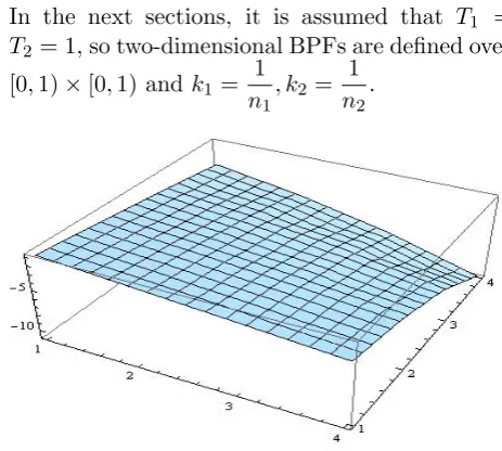
In the next sections, it is assumed that T1 =

T2= 1, so two-dimensional BPFs are defined over

[0,1)×[0,1) and k1 =

1 n1

, k2 =

1 n2

.

Figure 1: Approximate solutionn= 4

Figure 2: Approximate solutionn= 10

3 Method of solution

In this section we solve two-dimensional linear stochastic Volterra-Fredholm integral equation

1.2 using two-dimensional BPFs.

Approximating functions f(x, y), K1(x, y, s, t),

K2(x, y, s, t), K3(x, y, s, t) and g(x, y) with

(5)

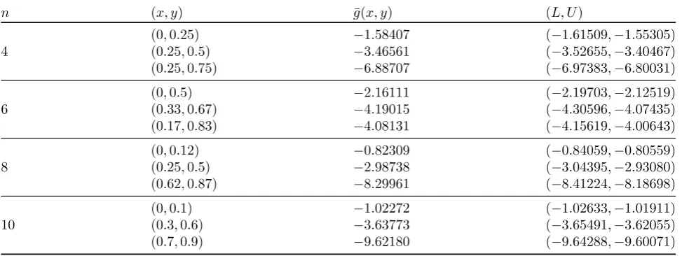
men-Table 1: The solutions mean with %95 confidence interval for above example.

n (x, y) g¯(x, y) (L, U)

(0,0.25) −1.58407 (−1.61509,−1.55305) 4 (0.25,0.5) −3.46561 (−3.52655,−3.40467) (0.25,0.75) −6.88707 (−6.97383,−6.80031)

(0,0.5) −2.16111 (−2.19703,−2.12519) 6 (0.33,0.67) −4.19015 (−4.30596,−4.07435) (0.17,0.83) −4.08131 (−4.15619,−4.00643)

(0,0.12) −0.82309 (−0.84059,−0.80559) 8 (0.25,0.5) −2.98738 (−3.04395,−2.93080) (0.62,0.87) −8.29961 (−8.41224,−8.18698)

(0,0.1) −1.02272 (−1.02633,−1.01911) 10 (0.3,0.6) −3.63773 (−3.65491,−3.62055) (0.7,0.9) −9.62180 (−9.64288,−9.60071)

tioned in Section2 gives

f(x, y) =FTΨ(x, y), (3.10)

K1(x, y, s, t) = ΨT(x, y)Γ1Ψ(s, t), (3.11)

K2(x, y, s, t) = ΨT(x, y)Γ2Ψ(s, t), (3.12)

K3(x, y, s, t) = ΨT(x, y)Γ3Ψ(s, t), (3.13)

and

g(x, y) =GT₁Ψ(x, y), (3.14)

where the vectorsF andG1 and matricesK1,K2

and K3 are BPFs coefficients of f(x, y), g(x, y),

K1(x, y, s, t), K2(x, y, s, t) and K3(x, y, s, t)

re-spectively and Ψ(x, y) is defined in2.3. In3.10,F is (n1n2×1) known vector, also in 3.11,3.12and 3.13, Γ1, Γ2 and Γ3 are (n1n2)×(n1n2) known

matrices but in 3.14, G1 is (n1n2×1) unknown

vector.

In Eq. 1.2 to approximate the first two-dimensional integral from3.11 and 3.14we get ∫ 1

0

∫ 1

0

= ∫ 1

0

∫ 1

0

ΨT(x, y)Γ1Ψ(s, t)ΨT(s, t)G1dsdt,

by using operational matrix D from Eq. 2.8 we have

= ΨT(x, y)Γ1

(∫ 1

0

∫ 1

0

Ψ(s, t)ΨT(s, t)dsdt )

×G1= ΨT(x, y)Γ1DG1 = (Γ1DG1)TΨ(x, y)

=GT₂Ψ(x, y),

where G2 is an (n1n2)-vector obtained from

Γ1DG1. Therefore the approximation of the

first dimensional integral with respect to two-dimensional BPFs may be compactly written as

∫ 1

0

∫ 1

0

K1(x, y, s, t)g(s, t)dsdt≃GT2Ψ(x, y).

(3.15) To approximate the second two-dimensional inte-gral in 1.2from Eqs. 3.12 and 3.14we get [1] ∫ y

0

∫ x

0

≃ ∫ y

0

∫ x

0

ΨT(x, y)Γ2Ψ(s, t)ΨT(s, t)G1dsdt

= ΨT(x, y)Γ2

(∫ y

0

∫ x

0

Ψ(s, t)ΨT(s, t)G1dsdt

) ,

from Eq. 2.5 follows

= ΨT(x, y)Γ2

(∫ y

0

∫ x

0

˜

G1Ψ(s, t)dsdt

)

= ΨT(x, y)Γ2G˜1

(∫ y

0

∫ x

0

Ψ(s, t)dsdt )

,

Using operational matrixP in Eq. 2.7 we have ∫ y

0

∫ x

0

≃ΨT(x, y)Γ2G˜1PΨ(x, y),

in which Γ2G˜1Pis an (n1n2)×(n1n2) matrix. Eq. 2.6 follows:

∫ y

0

∫ x

0

K2(x, y, s, t)g(s, t)dsdt≃GT3Ψ(x, y),

(6)

where G3 is an (n1n2)-vector with components

equal to the diagonal entries of matrix Γ2G˜1P.

Similarly to approximate the stochastic integral case in 1.2from Eqs. 3.13and 3.14 we get

∫ y

0

∫ x

0

K3(x, y, s, t)g(s, t)dB(s)dB(t)

≃ ∫ y

0

∫ x

0

ΨT(x, y)Γ3Ψ(s, t)ΨT(s, t)

×G1dB(s)dB(t) = ΨT(x, y)Γ3

× (∫ y

0

∫ x

0

Ψ(s, t)ΨT(s, t)G1dB(s)dB(t)

) ,

from Eq. 2.5 we have

= ΨT(x, y)Γ3

(∫ y

0

∫ x

0

˜

G1Ψ(s, t)dB(s)dB(t)

)

= ΨT(x, y)Γ3G˜1

(∫ y

0

∫ x

0

Ψ(s, t)dB(s)dB(t) )

.

By using operational matrix Ps in Eq. 2.9 we have

∫ y

0

∫ x

0

≃ΨT(x, y)Γ3G˜1PsΨ(x, y),

in which Γ3G˜1Ps is an (n1n2)×(n1n2) matrix.

Eq. 2.6follows: ∫ y

0

∫ x

0

≃GT₄Ψ(x, y), (3.17)

where G4 is an (n1n2)-vector with components

equal to the diagonal entries of matrix Γ3G˜1Ps. Applying Eqs. 3.10, 3.14, 3.15, 3.16 and 3.17 in Eq. 1.2we get

GT₁Ψ(x, y)≃FTΨ(x, y) +GT₂Ψ(x, y)

+GT₃Ψ(x, y) +GT₄Ψ(x, y). (3.18)

Replacing ≃with =, Eq. 3.18 gives

G1−G2−G3−G4=F. (3.19)

The equation 3.19 generate a system of (n1n2)

linear equations with (n1n2) unknown variable

which can be solved using Newton’s iterative method.

4 Numerical Example

In this section, the numerical example is given to demonstrate the applicability and accuracy of our method. For convenience we put n1 =n2 =nso

k1=k2 =

1 n.

Example 4.1 Consider the following linear two-dimensional stochastic Volterra integral equation of second kind:

g(x, y) =f(x, y)

+ ∫ 1

0

∫ 1

0

(x+y+t−s)u(s, t)dsdt

+ ∫ y

0

∫ x

0

(x+y+t−s)u(s, t)dsdt

+ ∫ y

0

∫ x

0

(x+y+t+s)u(s, t)dB(s)dB(t)

where

f(x, y) =x+y− 1 12xy(x

3_{+ 4x}2_y_{+ 4xy}2₊_y3_).

The solutions mean (¯g(x, y)) with %95 confidence interval (L, U) at the points that as for condition s ⩽ x < t ⩽ y are selected for the present method for 500 iterative of system 3.19 is shown in Table 1. The numerical example is carried out for selected grid points which are proposed by difference as (2−k, k = 4,6,8,10). In Figs. 1-2, three-dimensional graphs of the approximate solution for various values of arbitary positive integern are shown.

5 Conclusion

(7)

equation which corresponds to a system of linear equations with unknown coefficients. The illus-trative example is included to demonstrate the validity and applicability of the technique. Math-ematica has been used for computations.

References

[1] K. Maleknejad, S. Sohrabi, B. Baranji, Two-dimensional PCBFs: Application to nonlin-ear Volterra integral equations, Proceedings of the World Congress on Engineering 2009 Vol II WCE 2009, July 1 - 3, 2009, London, U.K.

[2] M. Khodabin, K. Maleknejad, M. Rostami, M. Nouri, Numerical approach for solving stochastic Volterra-Fredholm integral equa-tions by stochastic operational matrix, Com-puters and Mathematics with Applications 64 (2012) 1903-1913.

[3] K. Maleknejad, M. Khodabin, M. Rostami, Numerical solution of stochastic Volterra in-tegral equations by a stochastic operational matrix based on block pulse functions, Math-ematical and Computer Modelling 55 (2012) 791-800.

[4] K. Maleknejad, M. Khodabin, M. Ros-tami, A numerical method for solving m-dimensional stochastic It Volterra integral equations by stochastic operational matrix, Computers and Mathematics with Applica-tions 63 (2012) 133-143.

[5] Kuo, Hui-Hsiung, Introduction to stochastic integration, Springer Science+Business Me-dia, Inc. 2006.

[6] K. E. Atkinson, The numerical solution of integral equations of the second kind, Cam-bridge University Press (1997).

[7] A. J. Jerri,Introduction to integral equations with applications, John Wiley and Sons, INC (1999).

[8] S. Chen, G. Wang, M. Chien, Analytical modelling of piezoelectric vibration-induced micro power generator, Mechatronics 16 (2006) 379-387.

[9] H. J. Dobner, Bounds for the solution of hy-perbolic problems, Computing 38 (1987) 209-218.

[10] R. Farengo, Y. C. Lee, P. N. Guzdar, An electromagnetic integral equation appli-cation to microtearing modes, Phys. Fluids 26 (1983) 3515-3523.

[11] A. V. Manzhirov, On a method of solv-ing two-dimensional integral equations of ax-isymmetric contact problems for bodies with complex theology, J. Appl. Math. Mech. 49 (1985) 777-782.

[12] M. A. Rahman, A rigid elliptical disc-inclusion in an elastic solid, subjected to a polynomial normal shift, J. Elasticity 66 (2002) 207-235.

[13] H. Guoqiang, W. Jiong, Extrapolation of nystrom solution for two dimentional non-linear Fredholm integral equations, J. Comp. App. Math. 134 (2001) 259-268.

[14] H. Brunner, Collocation methods for Volterra integral and related functional equations, Cambridge University Press, 2004.

[15] H. Guoqiang, K. Itayami, K. Sugihara, W. Jiong, Extrapolation method of iterated col-location solution for two-dimentional nonlin-ear Volterra integral equations, Appl. Math. Comput. 112 (2000) 49-61.

[16] W. Xie, F. R. Lin,A fast numerical solution method for two dimensional Fredholm inte-gral equations of the second kind, App. Num. Math. 59 (2009) 1709-1719.

[17] S. Bazm, E. Babolian, Numerical solution of nonlinear two-dimensional Fredholm inte-gral equations of the second kind using Gauss product quadrature rules, Commun. Nonlin-ear Sci. Numer. Simult. 17 (2012) 1215-1223.

[18] G. Han, R. Wang, Richardson extrapolation of iterated discrete Galerkin solution for two-dimensional Fredholm integral equations, J. Comp. App. Math. 139 (2002) 49-63.

(8)

for solving nonlinear class of mixed Volterra-Fredholm integral equations, Math. Comp. Mode. 55 (2012) 1833-1844.

[20] E. Babolian, K. Maleknejad, M. Roodaki, H. Almasieh,Two dimensional triangular func-tions and their applicafunc-tions to nonlinear 2d Volterra-Fredholm equations, Comp. Math. App. 60 (2010) 1711-1722.

[21] S. Nemati, P. Lima, Y. Ordokhani, Numer-ical solution of a class of two-dimensional nonlinear Volterra integral equations using legender polynomials, J. Comp. Appl. Math. 242 (2013) 53-69.

[22] A. Tari, M. Rahimi, S. Shahmorad, F. Ta-lati, Solving a class of two-dimensional linear and nonlinear Volterra integral equations by the differential transform method, J. Comp. Appl. Math. 228 (2009) 70-76.

[23] P. Assari, H. Adibi, M. Dehghal, A meshless method for solving nonlinear two-dimensional integral equations of the second kind on non-rectangular domains using ra-dial basis functions with error analysis, J. Comp. Appl. Math. 239 (2013) 72-92.

[24] M. H. Reihani, Z. Abadi, Rationalized Haar functions method for solving Fredholm and Volterra integral equations, J. Comp. Appl. Math. 200 (2007) 12-20.

[25] F. Hosseini Shekarabi, K. Maleknejad, R. Ezzati, Application of two-dimensional Bernstein polynomials for solving mixed Volterra-Fredholm integral equations, African Mathematical Union and Springer-Verlag Berlin Heidelberg, http://dx.doi. org/10.1007/s13370-014-0283-6/. [26] G. P. Rao, Piecewise constant ortogonal

functions and their application to systems and control, Springer-Verlag, 1983.

[27] Z. H. Jiang, W. Schaufelberger, Block pulse functions and their applications in control systems, Springer-Verlag, 1992.

[28] C. H. Wang, Y.P. Shih, Explicit solutions of integral equations via block-pulse functions, Int. J. Syst. Sci., V13, pp. (1982) 773-782.

[29] K. Maleknejad, M. Shahrezaee, H. Khatami, Numerical solution of integral equations sys-tem of the second kind by block pulse func-tions, Appl. Math. Comput, 166 (2005) 15-24.

Mohsen Fallahpour was born in Karaj, Iran, in 1978. He is currently Ph.D. Student in IAU-karaj branch. Also he is one of the researcher in this university. He is now lecturer in the CFU-karaj campus, PNU-Nazaraabad, Islamic Azad University Karaj Branch and IAU-Hashtgerd.

I was born on September 4, 1969 in the city of Karaj. I receipt high school diploma in 1988 on math-ematics branch. In 1989, I suc-cessfully passed the university en-trance exam and started my aca-demic studies on the statistics in the Shahid Beheshti University in Tehran. In 1994, I continue my studies at MS level on the statistics in the same university. In 1998, I be-came a member of the board of department of mathematics in Islamic Azad University Karaj branch. In 2000, I emprise to obtain my Ph.D. on statistics in Sciences Research University Tehran branch.