VOLUME 40, ARTICLE 13, PAGES 319
,
358
PUBLISHED 21 FEBRUARY 2019
https://www.demographic-research.org/Volumes/Vol40/13/ DOI: 10.4054/DemRes.2019.40.13
Research Article
Population sex imbalance in China before the
One-Child Policy
Kimberly Singer Babiarz
Paul Ma
Shige Song
Grant Miller
© 2019 Kimberly Singer Babiar et al.
This open-access work is published under the terms of the Creative Commons Attribution 3.0 Germany (CC BY 3.0 DE), which permits use, reproduction, and distribution in any medium, provided the original author(s) and source are given credit.
1 Introduction 320
2 Background and conceptual framework 323
2.1 Sex selection in China in recent history 323
2.2 A simple conceptual framework for fertility decline and sex selection
325
3 Data and methods 325
3.1 Data 325
3.2 Methods 327
3.2.1 Graphical analysis 327
3.2.2 Multivariate statistical analysis 328
4 Results 329
4.1 Graphical analysis 329
4.1.1 Sex ratios at birth 329
4.1.2 Sex ratios at ages 1–5 330
4.2 Statistical analysis 331
5 Data quality and possible under-reporting of living girls 332
5.1 Adoption and survey design 333
5.2 Empirical assessment of under-reporting 334
6 Discussion 336
References 338
Population sex imbalance in China before the One-Child Policy
Kimberly Singer Babiarz1
Paul Ma2
Shige Song3
Grant Miller4
Abstract
OBJECTIVE
Most research on population sex imbalance in China has focused on the One-Child Policy era. However, because much of China’s fertility decline occurred during the 1970s, we investigate the possibility that sex ratios began rising during this period (as predicted by theory) before the One-Child Policy.
RESULTS
Analyzing sex ratios between 1960 and 1987 by birth order and sibship sex composition, we find that among the subset of couples expected to have the greatest demand for sons (those at higher parities without previous sons), sex ratios at birth reached 115–121 boys per 100 girls during the 1970s – implying approximately 840,000 to 1,100,000 girls missing from Chinese birth cohorts during the 1970s. Importantly, these results do not appear to be driven by differential under-reporting of living girls, or instances of adoption. Given the absence of ultrasound technologies prior to 1979, they imply the presence of postnatal sex selection in China during the 1970s.
CONTRIBUTION
Our work makes several important contributions to existing literature. First, we focus on the subset of couples among whom the demand for sons is predicted to be the strongest: higher parity couples not yet having a boy. Second, we estimate sex ratios by single year of age (from birth to age 4), distinguishing differential rates of infant death from more gradual neglect of girls as they age throughout childhood. Third, we
1 Stanford University, Stanford, USA. Email:[email protected].
2 Carlson School of Management, University of Minnesota, Minneapolis, USA.
3 Queens College and CUNY Institute for Demographic Research, The City University of New York, New
York City, USA.
combine graphical and multivariate statistical analyses to test for meaningfully imbalanced sex ratios. Finally, we measure potential irregularities in the reporting of living girls, including the adoption of girls, and we generate new estimates of unreported females.
1. Introduction
China’s sex ratio at birth5 rose dramatically throughout the 1980s (Banister 2004; Coale and Banister 1994). A large literature estimates that between 8.5 and 9.2 million females are missing from Chinese cohorts born between 1980 and 2000 – presumably the result of sex-selective abortion and childhood neglect (Almond, Li, and Zhang 2017; Cai and Lavely 2003; Chen, Li, and Meng 2013; Ebenstein 2014; Jiang et al. 2012; Tuljapurkar, Li, and Feldman 1995). Given parental preferences for sons,6 the One-Child Policy (in 1980) and the rapid diffusion of ultrasound technologies capable of detecting fetal sex (during the early 1980s (Chen, Li, and Meng 2013)) are together generally considered responsible for China’s ‘missing women’ that emerged during the 1980s and later (Banister 2004; Das Gupta 2005; Das Gupta and Li 1999; Ebenstein 2014; Ebenstein and Leung 2010; Johansson and Nygren 1991).7
However, demographic and economic theory suggest that as fertility declines in populations preferring sons, sex ratios will rise (Das Gupta and Bhat 1997; Das Gupta and Li 1999; Jayachandran 2017) – and strikingly, most of China’s fertility decline occurred during the 1970s under China’s first national birth planning policy, the “Later, Longer, Fewer” campaign. The campaign sought to reduce the country’s birth rate by raising the minimum age at marriage (“later”), lengthening birth intervals (“longer”), and reducing fertility to a maximum of three births per couple (“fewer”). In rural areas (accounting for over 80% of the Chinese population in 1970), the total fertility rate (TFR) fell from 6.4 in 1970 to about 3 by 1979 (and from 3.2 to 1.4 during this period in urban areas; Figure 1) (Banister 2004; Cai and Lavely 2003; Coale and Banister 1994). This decline is among the most rapid documented reductions in fertility in global
5 The sex ratio at birth is defined as the number of boys born per 100 girls.
6 Scholars have linked China’s skewed sex ratio to son preference and patriarchal traditions emphasizing the
role of sons in elder care and lineage (Coale and Banister 1994; Ebenstein 2014; Ebenstein and Leung 2010; Jayachandran 2015).
7 Coale and Banister (1994) find that average sex ratios over 5-year intervals among third and fourth order
history.8 Nonetheless, existing studies of China’s fertility decline prior to 1980 are largely descriptive and report only modest sex imbalance (with unknown quantitative/statistical significance (Banister 2004; Cai and Lavely 2003; Coale and Banister 1994; Das Gupta and Li 1999; Jiang et al. 2012; Johansson and Nygren 1991).
Figure 1: Total fertility rate decline in China 1950–1984
Note: Total fertility rates (TFR) are calculated as the sum of age-specific fertility rates observed in a given calendar year. Panel A is reproduced using TFRs calculated in Chen (1984) from the 1982 National Sample Survey of Fertility and Contraception (the one-per-thousand survey) and Panel B shows highly consistent TFRs calculated using birth records in the 1988 National Sample Survey of Fertility and Contraception (the two-per-thousand survey).
8 Other rapid declines in fertility have occurred in Iran (where the total fertility rate fell from about 6.5 in
Using historical fertility data (retrospective fertility histories in China’s 1988 Two-per-Thousand National Sample Survey of Fertility and Contraception), this paper investigates the theoretical prediction that, despite efforts to prevent sex selection, sex ratios at birth began rising as China’s total fertility rate plummeted during the 1970s – earlier and to higher levels than previously established. In doing so, it makes several important contributions to the existing literature. First, unlike previous work, it is able to isolate and study the subset of couples among whom the demand for sons is predicted to be the strongest: higher parity couples not yet having a boy (Arnold and Liu 1986; Das Gupta 2005; Ebenstein 2014).9 Most previous studies use population census data in which births cannot be distinguished by parity and sex composition of older siblings.10 Second, in estimating sex ratios by single year of age in each year (rather than pooling birth cohorts), it is able to distinguish differential rates of infant death during the first year of life (due either to differential neglect or possible infanticide) from more gradual neglect of girls as they age throughout childhood.11 Third, it combines graphical and multivariate statistical analyses to test for meaningfully imbalanced sex ratios at birth using a sample restricted to years prior to the introduction of ultrasound technology in each province. This contribution is particularly important for analysis based on fertility histories (in which we know the ages at which girls become ‘missing’) rather than census counts. Fourth, it pays special attention to potential irregularities in the reporting of living girls, including the adoption of girls, generating new estimates of female under-reporting.
Consistent with theoretical predictions, we find that among third and higher parity births to couples without a surviving son,12 sex ratios rose as high as 115–121 boys per 100 girls during the 1970s – higher than previously established. Our analysis implies that, although rare in absolute terms (accounting for less than 0.5% of births) and concentrated among a narrow subset of couples, approximately 840,000–1,100,000 girls are missing from Chinese birth cohorts during the 1970s. Moreover, we find that these missing girls are unlikely to be explained by systematic under-reporting of living children or instances of adoption.
9 We use the number of previous live births to define parity groups and birth orders.
10 Coale and Banister (1994) show sex ratios by 5 year birth cohort among pooled first and second order
births, and pooled third and fourth order births. The authors compare the sex ratios of births by within-sex birth order among babies born in 5 year birth cohorts, showing that girls are more likely to be missing when they have older sisters compared to boys when they have older brothers. However, the authors do not measure the absolute sex ratio among births in each year by birth order and sibship sex composition.
11 Several studies using census counts show differential mortality rates over time or sex ratios at birth among
pooled birth cohorts, neither approach permitting nuanced analysis of the age at which girls are missing from populations Cai and Lavely 2003; Coale and Banister 1994).
12 Throughout this study, we characterize the sex composition of older siblings surviving at the time of the
This paper proceeds as follows. Section 2 provides a brief background on sex ratios over time in China and presents a stylized model of fertility decline and sex selection when there is son preference. Section 3 describes our data sources and methodology, and Section 4 presents our primary results. Section 5 then assesses data quality and investigates the possibility of differential under-reporting of female births, and Section 6 concludes.
2. Background and conceptual framework
2.1 Sex selection in China in recent history
Historical population research provides rich qualitative evidence of high sex ratios during China’s Imperial period, extending into the first half of the 20th century (King 2014; Mungello 2008; Wolf and Huang 1980). This work generally attributes the persistence of male-biased sex ratios to a strong preference for sons rooted in patriarchal traditions (Das Gupta and Li 1999; Ebenstein 2014; Ebenstein and Leung 2010; Greenhalgh 1988). Although there is evidence of advocacy against the practice (Mungello 2008), families of all social strata used female infanticide and abandonment to control family size and composition (Greenhalgh 1988; King 2014; Langer 1973; Lee and Wang 1999b; Mungello 2008). Some accounts suggest that 10% of female births may have ended this way, with rates as high as 40% reported among some subgroups (documented among Imperial families during specific periods, for example) (King 2014; Lee and Wang 1999a, 1999b).
The first population censuses conducted in the People’s Republic of China (in 1953 and 1964) provide evidence that sex ratios were high during the early 20th century, but then fell around the time of the 1949 communist revolution. The ratio of men to women born during the 1920s and 1930s appears to have ranged between 107.3 and 113.6, peaking during the 1940s at 112.7–117.7 in 1953 (Banister 1991).13 Shortly after the communist revolution, China’s sex ratio at birth then appears to have fallen to naturally occurring levels below 107 (Banister 1991).14 Some research suggests this was due to efforts to promote gender equality and discourage ‘feudal’ attitudes toward
13 Although it is not possible to distinguish if these high sex ratios emerged at birth or reflect differential
mortality throughout childhood and early adulthood, qualitative records suggest that much of this imbalance may have emerged around the time of birth (Song 2012).
14 The biologically ‘natural’ sex ratio at birth is generally believed to be 105–107 (Grech, Savona-Ventura,
daughters, however son preference persisted as sons continued to ensure lineage continuation and provide greater economic security compared to daughters.15
From ‘balanced’ levels early in the communist era, existing studies then focus on the rapid resurgence of male-biased sex ratios beginning in 1980 under the One-Child Policy (and coincident with the diffusion of ultrasound technology across the country). A large body of research suggests that between 8.5 and 9.2 million girls are missing from cohorts born between 1980 and 2000 – generally at very young ages (Cai and Lavely 2003; Jiang et al. 2012). Specifically, in years 1990 and 1995, sex ratios at birth reached estimated levels of 111.8 and 116.6 (Banister 2004). Unlike earlier years, many studies argue that the diffusion of ultrasound technology (and the ability to detect fetal sex) during this period enabled families to selectively abort girls – effectively making sex selection ‘easier’ or less costly (Banister 2004; Cai and Lavely 2003; Chen, Li, and Meng 2013; Coale and Banister 1994).16
Little previous research reports evidence (or statistically significant evidence) of rising sex ratios during the 1970s – prior to the One-Child Policy and diffusion of ultrasound technology. Instead, many past studies are descriptive or focus on establishing ‘baseline’ population sex ratios to then quantify dramatic increases under the One-Child Policy (Banister 2004; Cai and Lavely 2003; Das Gupta 2005; Jiang et al. 2012; Johansson and Nygren 1991).17 Nonetheless, modern China’s most dramatic fertility decline occurred during this decade. Rural China’s TFR fell by more than half, from approximately 6.4 in 1970 to about 3 in 1979 (Banister 2004; Cai and Lavely 2003; Coale and Banister 1994). Demographic and economic theory suggest that given preferences for sons, rapid fertility decline (whatever the cause – demand- or supply-driven) should be accompanied by rising sex ratios (Almond, Li, and Zhang 2017; Becker 1960, 1991; Das Gupta and Bhat 1997; Das Gupta and Li 1999; Jayachandran 2017; Jayachandran and Kuziemko 2010; Schultz 1985). Additionally, this increase in male-biased sex ratios should be concentrated among couples with the greatest demand for sons. Although individual and couple/household preferences are not observed, this group should disproportionately include higher parity couples without a surviving son.
15 Despite the collective organization of agriculture, families remained patriarchal in nature. Property and
lineage was passed through the male line and married couples lived with and cared for the husband’s parents. Males were also awarded more work points and greater rations compared to female family members and offered greater opportunities for sociopolitical advancement through military or political careers (Arnold and Liu 1986; Ebenstein 2014; Ebenstein and Leung 2010; Greenhalgh 1988; Greenhalgh and Li 1993).
16 Media archives and public policy statements discussing female infanticide in the early 1980s suggest that
the practice was ongoing in some areas (Banister 1991; Greenhalgh and Winckler 2005; White 2000, 2009).
17 Coale and Banister (1994) show sex ratios by 5 year birth cohort among pooled first and second order
In this next section, we present a stylized conceptual framework for understanding decision-making about sex selection as fertility rates decline.
2.2 A simple conceptual framework for fertility decline and sex selection
In this section, we briefly summarize how fertility constraints theoretically affect sex selection behavior (as empirically documented by Das Gupta and Bhat (1997) and Guilmoto (2009), for example). As Das Gupta and Bhat (1997) note, the key necessary assumption is that when fertility declines, the desired family size falls more rapidly than the target number of sons (among couples with some form of son preference).18 Put differently, the decline in the demand for daughters outpaces the decline in demand for sons, increasing sex selection pressure (Li, Feldman, and Tuljapurkar 2000). As fertility constraints tighten, the opportunity cost of having an unwanted girl then rises (because the probability of not having the target number of sons increases). Consequently, couples for whom the opportunity cost of a girl exceeds the cost of sex selection will sex select (prenatally or postnatally – in our case, because we only study province-years in which ultrasound technology was not available, postnatally) (Anukriti 2016; Ebenstein 2011; Lin, Liu, and Qian 2014). In the aggregate the consequences for sex ratios are unambiguous: an increase in the cost of children leads not only to smaller family sizes, but also greater neglect of daughters – and hence rising sex ratios. We provide a simple formal conceptualization of this decision in the online supplemental material.
3. Data and methods
3.1 Data
We use China’s 1988 National Sample Survey of Fertility and Contraception (also known as the “two-per-thousand” fertility survey), which collected data from 417,518 women in 30 Chinese provinces and municipalities.19 Conducted by the State Family
18 Households are assumed to have a target number of children they would like to have taking the full cost of
having and raising children into account – a target which is independent of their desire for sons. Importantly, we distinguish the “desired” or “target” number of children couples would like to have from standard demographic measures such as the ‘ideal number of children,’ ‘desired total fertility,’ and ‘wanted total fertility.’ The online supplemental material provides additional detail.
19 Provinces and municipalities surveyed include: Anhui, Beijing, Fujian, Gansu, Guangdong, Guangxi,
Planning Commission of China, the survey interviewed a representative sample of ever-married Chinese women ages 15–57 from approximately 14,000 sampling units (neighborhood small group for cities and village small group in rural areas) across the country. This survey was an expanded version of the 1982 National Sample Survey of Fertility and Contraception (the “one-per-thousand” fertility survey) and is generally believed to be accurate and good quality (Coale 1984; Coale and Banister 1994; Zhang and Zhao 2006).20
For the purpose of our study, the 1988 “two-per-thousand” fertility survey has several important advantages over its predecessor (the “one-per-thousand” fertility survey) as well as to China’s national population censuses. The “one-per-thousand” survey also collected fertility histories, but this did not include information about infant and child deaths, preventing analysis of sex-specific mortality as children aged. China’s 1982 and 1990 population censuses have been widely used to study population sex imbalance (Banister 2004; Cai and Lavely 2003; Das Gupta and Li 1999; Ebenstein 2014; Jiang et al. 2012), but they also lack information about child deaths – and importantly (given our focus), they do not contain sufficient information to estimate sex ratios by birth order, sex composition of previous births, and year. These features may be critical for understanding the early emergence of sex imbalance in the Chinese population (Muhuri and Preston 1991).
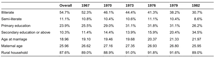
Each sampled woman in the 1988 “two-per-thousand” fertility survey provided detailed information about her complete fertility history, including all pregnancies ending in miscarriage, abortion, stillbirths, and live births. For each live birth, the survey collected the date of birth, sex of the child, whether or not the child was alive at the time of the survey, and if not, the date that the child died. The survey also recorded socioeconomic information about each mother, including her own date of birth, ethnicity, province of residence, and urban/rural residency status (hukou). Table 1 provides descriptive statistics of mothers having births in selected years during the period of study, and Appendix Table A-1 provides the sample size of birth records used.
Liaoning, Ningxia, Qinghai, Shaanxi, Shanghai, Shandong, Shanxi, Sichuan, Tianjin, Xinjiang, Yunnan, Zhejiang.
Table 1: Characteristics of mothers by year of delivery, 1967–1983
Overall 1967 1970 1973 1976 1979 1982 Illiterate 54.7% 52.3% 46.1% 44.4% 41.3% 38.2% 30.7% Semi-literate 11.1% 10.8% 10.4% 10.6% 11.1% 10.4% 8.6% Primary education 23.9% 25.5% 29.0% 31.1% 31.8% 31.1% 26.2% Secondary education or above 10.3% 11.4% 14.4% 13.9% 15.9% 20.4% 34.5% Age at marriage 18.96 19.10 19.46 19.68 20.37 21.33 21.97 Maternal age 25.96 26.62 27.16 27.35 26.93 26.80 25.95 Rural household 87.6% 89.0% 88.9% 91.0% 91.8% 91.6% 89.0%
Source: State Family Planning Commission of China, 1988 Two-per-Thousand National Sample Survey of Fertility and Contraception.
3.2 Methods
3.2.1 Graphical analysis
We conduct both graphical and multivariate statistical analysis of population sex imbalance by year of birth, birth order, and sex composition of previous births (defined as the presence/absence of a living older male sibling at the time of the relevant birth – henceforth termed “sibship sex composition”). Our graphical analysis uses each birth, combined with birth records of all children born to the same mother, to determine both birth order and sibship sex composition.21 We then calculate sex ratios (or the number of males for every 100 females) at birth and at each subsequent year of age up to age 5 by year of birth, birth order, and sibship sex composition between 1962 and 1987.22 Finally, we plot these sex ratios (at birth and at each year of age up to 5) over time.
Given the lack of prenatal sex determination technology prior to the early 1980s (Chen, Li, and Meng 2013), we interpret sex ratios at birth above the naturally occurring level of 105–106 (Grech, Savona-Ventura, and Vassallo-Agius 2002; Johansson and Nygren 1991; Sen 1990) prior to the 1980s to reflect postnatal selection in favor of males – around the time of birth or in the first year of life, subject to reporting considerations examined in Section 5.
21 As Footnote 11 describes, our results are insensitive to an alternate definition of sibship sex composition
using indicators for whether or not any preceding birth was a boy, regardless of survival (results available on request).
3.2.2 Multivariate statistical analysis
We also use Ordinary Least Squares (OLS) regression models to estimate the joint marginal relationship of birth year, birth order, and sibship sex composition with the marginal probability that a given birth is male (relative to 1967). Specifically, we estimate models of the following general form separately for birth order p births to mothersiin yearsy, grouping third- and higher-order births together:
= + + ℎ
+ ∑ ℎ × + ∑ + + , (1)
where is a dichotomous indicator variable for whether or not an orderp child born to motheri living in provincej in yeary was male, ℎ is a dichotomous indicator for birth in year y, is a dichotomous indicator for whether or not mother i had a previous son surviving to year y, and is avector of k maternal characteristics (indicators for residence in an urban area and mothers’ educational attainment strata, as well as mother’s age at marriage). In addition to main effects, we
also include all two-way interactions between ℎ and . Equation 1
also includes provincial fixed effects( ), which control for unobserved time-invariant differences across provinces. Appendix Tables A-3–A-4 show that our results are robust to the exclusion of urban and semi-urban populations.
We use linear probability models to allow for consistent fixed effects estimation while avoiding concerns about incidental parameters (Neyman and Scott 1948). Appendix Table A-5 reports results obtained using probit regressions, yielding comparable findings. We compute Huber–White robust standard errors clustered at the province level, relaxing the assumption that error terms are identical and independently distributed (i.i.d.) across provinces. The resulting estimates of – allow us to calculate the probability of being male in excess of biologically expected levels as a linear combination of year of birth, birth order, sibship sex composition, and all interactions among them. To draw conclusions about what these estimates imply about the prevalence of postnatal sex selection, we restrict our analyses to years before the introduction of ultrasound technology in each province (Chen, Li, and Meng 2013).23
23 Data on ultrasound availability at the county-year level is from Chen and coauthors (2013), who digitize
4. Results
4.1 Graphical analysis
4.1.1 Sex ratios at birth
Figure 2 plots sex ratios at birth by year, birth order, and sibship sex composition for each year between 1962 and 1987. At all parities, regardless of previous sons, sex ratios at birth were largely stable throughout the 1960s and early 1970s, oscillating around the natural rate. This is consistent with past analyses suggesting little sex imbalance at birth prior to the 1980s at this level of aggregation (Banister 2004; Coale and Banister 1994; Das Gupta and Li 1999; King 2014).
Figure 2: Sex ratio at birth by birth order and sibship sex composition in China 1962–1987
Note: Figure shows reported sex ratio at birth, by birth order and sibship sex composition. Sex ratio is calculated as the number of male births divided by the number of female births in each parity and sibship sex composition category.
Source: 1988 National Sample Survey of Fertility and Contraception.
However, consistent with theoretical predictions, as China’s total fertility rate declined during the 1970s, the sex ratio of higher-order births depends critically on sibship sex composition.24 Among mothers with at least one surviving son, this
24 We conceptualize household fertility decision-making to depend on the sex composition of older surviving
trajectory is also flat, remaining close to the natural rate throughout the 1970s. However, for mothers without sons, the sex ratio at birth rises rapidly throughout the decade – and does so earlier at higher parities. Among third- and higher-order births, the sex ratio among mothers without previous sons rises as high as 120.8 in 1977 (and 115.6 in 1979).25 This increase in the probability of male births at higher parities among women without living sons then continues throughout the 1980s as fertility declines further, the One-Child Policy is introduced, and ultrasound technologies become available.
4.1.2 Sex ratios at ages 1–5
Figure 3 repeats the graphical analysis shown in Figure 2 for sex ratios at birth and each single-year age interval up to age 5. Births of each order are shown in separate panels. Relative to the sex ratio at birth within a given subgroup, sex ratios at subsequent ages up to age 5 generally change little. One exception is the modest increase at third- and higher-order births among households without a previous son. Within this subgroup, the sex ratio rises at age 1 by approximately 2–3 additional boys per 100 girls. The stability (and in some cases, increase) in age-specific sex ratios from birth up to age 5 contrasts with biologically higher rates of mortality among boys at all ages (Coale 1991). Overall, Figure 3 suggests that the majority of China’s population sex imbalance during the 1970s occurred around the time of birth.
instead using the sex composition of previous births (specifically, the presence of a previous male birth), regardless of survival to the time of a fertility decision. These results are available upon request.
25 Previous research reports average sex ratios over 5-year intervals at third and fourth parities, regardless of
Figure 3: Sex ratio at age 1–4 by birth order and sibship sex composition in China 1962–1987
Note: Figure shows reported sex ratio at ages 1–4, by birth order and sibship sex composition. Sex ratio is calculates as the number of male children divided by the number of female children reaching each relative age in each birth order and sibship sex composition category.
Source: 1988 National Sample Survey of Fertility and Contraception.
4.2 Statistical analysis
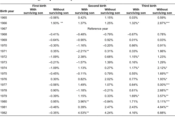
The results of our statistical analysis (Table 2) are consistent with Figure 2.26 We estimate the marginal probability that a child born is male by birth year, birth order, and sibship sex composition, calculating these probabilities using coefficient estimates obtained from Equation 1. Adjusting for observable maternal characteristics as well as provincial and birth year fixed effects, the probability that a first-born child is male does not rise during the 1970s relative to 1969 (the reference year, in which it is 51.5% – approximately the biologically expected rate). After a woman’s first child, sibship sex composition then becomes a key determinant of the probability of a male birth. With few exceptions, the probability that a child born to a woman with at least one older living son is statistically indistinguishable from the biologically expected probability throughout the 1970s. However, among women without surviving sons, a third- or higher-order child born after 1973 is 2–5 percentage points more likely to be a male (implying sex ratios at birth of 113–129).27
26 Because we restrict our statistical analysis to province-year observations in which ultrasound technology
was not available, Table 2 shows results for years 1965–1982.
Table 2: Marginal probability of a male birth, conditional on live birth
First birth Second birth Third birth Birth year With
surviving son Without surviving son With surviving son Without surviving son With surviving son Without surviving son 1965 –0.56% 0.42% 1.15% 0.03% 0.59% 1966 1.93% ** 1.37% 1.25% 1.32%* 2.87%*** 1967 Reference year
1968 –0.41% –0.48% –0.79% –0.67% 0.78% 1969 –0.64% –0.90% 0.92% 0.01% 0.03% 1970 –0.30% –1.16% –0.20% 0.66% 0.91% 1971 0.35% –2.21%** 0.31% 0.33% 1.86% 1972 –1.09% 2.38% 0.68% 1.15%* 1.23% 1973 –0.21% –1.57% 1.39% 0.16% 1.29% 1974 –1.09% 1.13% 0.27% 1.17%* 2.12%* 1975 –0.45% –0.11% 0.79% 0.55% 1.69%** 1976 0.30% 0.82% 2.02% 0.77% 1.93%* 1977 –0.56% 1.49% 1.07% 0.64% 5.00%*** 1978 0.90% –1.18% –0.21% 0.61% 2.68%** 1979 –0.39% 1.15% 0.33% 1.69%* 3.57%** 1980 0.95% 3.96%** –0.84% 1.71% 5.11%*** 1981 –0.46% 0.39% 2.47% 2.43% 4.84%** 1982 –0.35% 4.53%** 4.24% 4.16% 6.88%
Note: Each cell contains marginal probability that a birth occurring in each year, birth order, and sibling sex composition category is male. Marginal probabilities are calculated from coefficients estimated using OLS regressions (estimated separately for births of each order) of an indicator for a male birth on indicators for birth year and the sex composition of older siblings, as well as all two - way interactions between birth year and sibship sex composition. We control for residence in urban area, mother's educational attainment strata, mother's age at marriage, and time-invariant province fixed effects. Huber–White robust standard errors are clustered at the province level. * p<0.10, ** p<0.05, *** p<0.001.
Source: 1988 National Sample Survey of Fertility and Contraception.
5. Data quality and possible under-reporting of living girls
Both true sex selection and under-enumeration of living children is well documented in the demography literature for Chinese birth cohorts from the 1980s and 1990s (Cai and Lavely 2003; Goodkind 2011; Merli and Raftery 2000; Zeng 1996; Zeng et al. 1993; Zhang and Zhao 2006). However, there is little existing evidence for birth cohorts from the 1970s. On one hand, penalties for violating fertility regulations were less severe prior to the One-Child Policy – and hence incentives for hiding unsanctioned births from enumerators were weaker. On the other hand, however, infant deaths may have been unreported in official registries at higher rates in earlier years for simple administrative reasons related to bureaucratic inefficiency (Coale and Banister 1994; Merli 1998). Some suggest that on balance, relative to later birth cohorts, the degree of under-enumeration of living children born during the 1970s was substantially less (Coale 1984; Coale and Banister 1994; Zeng et al. 1993). To the best of our knowledge, however, no study has empirically evaluated the degree of under-reporting of births from the 1970s in the 1988 “two-per-thousand” survey – including under-reporting by birth order and under-under-reporting of girls relative to boys.
We use several methods to investigate the extent to which unreported girls lived beyond infancy as unregistered and unenumerated children, which we present below.
5.1 Adoption and survey design
Before applying established demographic methods for assessing under-reporting of living girls, we first briefly consider how the design of the “two-per-thousand” survey (and enumerator instructions) handles adoption – a specific potential form under-reporting.28 Survey enumerators were instructed to ensure that adopted children (“adopted-in”) were not listed in pregnancy histories as ‘own children’ – and also to ensure that children given up for adoption (“adopted-out”) were included in these histories. To accomplish this, the survey included cross-validation measures designed to explicitly handle adoptions in this way (SFPC 1988).29 Although we are of course unable to verify how enumerators conducted fieldwork in practice, systematic
under-28 If boys adopted into families are reported in our survey’s fertility records, or if girls who were given up for
adoption are not reported, then the sex ratios that we compute would be inflated.
29 Specifically, before asking questions about each pregnancy, enumerators were instructed to ask how many
reporting of children adopted-out (along with other types of under-reporting) would be captured by our analyses below in Section 5.2.
5.2 Empirical assessment of under-reporting
We then test empirically for systematic under-reporting of living children who could have been adopted-out, or otherwise hidden from enumerators, using three approaches. The first two modify methods used to evaluate the quality of the 1982 “one-per-thousand” national fertility survey, and the third compares the 1988 “two-per-“one-per-thousand” national fertility survey with the 1982 survey (which is generally considered good quality) (Banister 2004; Ní Bhrolcháin and Dyson 2007; Coale 1991; Coale and Banister 1994).
First, following Coale and Banister (1994), we investigate the extent to which possibly unreported female births in the 1988 “two-per-thousand” survey ‘reappear’ as adult women in China’s population censuses, focusing on those births most likely to be underreported. We compare sex ratios at birth (number of male births for each 100 female births) for each birth cohort reported in the 1988 fertility survey with sex ratios for the same birth cohorts as reflected in the 1% micro samples of the 1982 and 1990 censuses. From cross-sectional census microsamples, we reconstruct sex ratios at birth by adjusting population counts for age- and sex-specific mortality rates, using a reverse survival method.30 We find that sex ratios at birth in the 1988 fertility survey are consistent with mortality-adjusted sex ratios observed among the same birth cohorts in both the 1982 and 1990 population censuses (Appendix Figures A-1–A-2 and Appendix Table A-6).
To the extent possible, we also investigate the degree to which higher birth order girls (who may have been alive but disproportionately under-reported in fertility histories) are more likely to appear in later population censuses than higher birth order boys. Specifically, we use the same approach described above, stratifying by both birth order sibship sex composition.31 Due to data requirements, we focus on birth cohorts
30 Mortality rates are derived from three sets of life tables. These are: 1) life tables presented in Coale (1984),
which interpolate between the 1964 and 1982 censuses; 2) life tables published in Banister (1991), which use China’s Cancer Epidemiology Study of deaths between 1973–1975; and 3) life tables based directly on the 1982 population census (Jiang, Zhang, and Zhu 1984). For all mortality rate adjustments, we necessarily assume that age- and sex-specific morality rates were stable over the period of study.
31 Because birth order is not directly reported in the population censuses, we reconstruct birth order and
born between 1975 and 1979 in the 1990 census, adjusting for mortality using birth order-, age-, and sex- specific mortality rates derived from the 1988 “two-per-thousand” survey.32 We find that girls born at higher parities and with no older brothers – precisely the circumstances under which sex selection is predicted to be strongest – are not more likely to reappear as adults in future censuses (i.e., we find no evidence of differential under-reporting by birth order and sex composition of previous births) (Appendix Figure A-3 and Appendix Table A-7).
Second, following Coale (1991), we use the 1988 “two-per-thousand” survey to calculate the age-specific rate at which women deliver male and female babies in each year. We then apply these fertility rates by maternal age and child sex (simultaneously) to age-specific population counts of women reported in population census microsamples (interpolated between the 1964 and 1982 censuses), yielding an estimate of the total number of boys and girls born in each calendar year. We then compare the estimated number of male and female births implied by these calculations to the actual number of individuals in each birth cohort in the 1982 and 1990 censuses to estimate the degree of underreporting for boys and girls by birth cohort in the 1988 fertility survey. We find that although females are slightly more likely to be unreported than males, the difference in rates remains relatively constant over time – and in fact decreases during the late 1970s (Appendix Figure A-4). For underreporting of surviving females to confound our main estimates of missing girls, they would need to increase relative to underreporting of males over time.
Third, we investigate the consistency of the 1988 “two-per-thousand” survey with its predecessor, the 1982 “one-per-thousand” survey (which others have shown to be good quality (Coale 1984)). To do so, we account for demographic changes between survey years by creating a matched sample of women across surveys. Specifically, for every woman in the “one-per-thousand” survey, we identify a woman in the “two-per-thousand” survey with the same characteristics,33 pooling matched observations from both surveys together. We then regress, separately, (1) the reported number of children (male and female combined), (2) the reported number of male children, and (3) the reported number of female children on a dichotomous indicator variable for which survey the observation was drawn from. The results imply that the number of children (male and female combined) recorded in the 1988 “two-per-thousand” survey is 0.026
order, and sibship sex composition), we focus on birth cohorts from the second half of the 1970s (1975– 1980).
32 Mortality rates from the 1988 “two-per-thousand” survey are shown to be consistent with life-table sources
in Appendix Figures A-1–A-2 and Appendix Table A-6.
33 Individuals in each survey are matched using five individual-level characteristics: birth cohort, urban/rural
fewer than in the 1982 survey [95% CI: 0.014 – 0.037]. Analogous estimates by sex imply 0.0164 fewer male births [95% CI: 0.010 – 0.023] and 0.009 fewer female births [95% CI: 0.003 – 0.016] in the 1988 survey. Overall, these results suggest a small degree of underreporting in the 1988 “two-per-thousand” survey relative to the 1982 survey. However, because underreporting is, to a small extent, more severe for male births than for female births, the implication is that our estimates of sex ratios at birth during the 1970s may be biased downwards.
6. Discussion
Guided by theory and previous literature, this paper uses fertility history data and a combination of graphical and statistical methods to investigate the possibility of previously undocumented sex imbalance at birth during China’s sharp fertility decline throughout the 1970s. Analyzing sex ratios at birth by both birth order and sibship sex composition (simultaneously), we find that among couples predicted to have the greatest demand for sons (third and higher parity births to couples not yet having a boy), sex ratios rose as high as 115–121 boys per 100 girls during the 1970s. Importantly, this finding does not appear to be fully explained by under-reporting of female births or the adoption of girls. It also cannot be explained by prenatal sex selection because we study only births prior to the introduction of ultrasound technology.
Infanticide and postnatal neglect has a long and well-documented history in many cultures, including China during the late Imperial period and during times of political and economic instability in the 20th century (Das Gupta and Li 1999; Greenhalgh and Winckler 2005; King 2014; Langer 1973; Lee and Wang 1999b; Mungello 2008; White 2009; Wolf and Huang 1980). This paper provides quantitative measurements of the practice during the 1970s among a small, but quantitatively important, subset of couples.34
Overall, our statistical analysis implies that, although rare (accounting for about 0.5% of births) and concentrated among higher-order births to families without surviving sons, approximately 1.1 million girls are missing from Chinese cohorts born during the 1970s.35 Our graphical analysis using unadjusted data (integrating under the curves shown for sex ratios at birth by birth order and sibship sex composition) yields a comparable estimate of 844,000 missing girls. Importantly, because these male-biased
34 This is consistent with ethnographic reports of incidents of infanticide in the early 1980s (Greenhalgh and
Winkler 2005; White 2006).
35 See online supplemental material for detailed calculations of the estimated number of missing girls during
sex ratios at birth emerge prior to the introduction of ultrasound (Chen, Li, and Meng 2013), they cannot be explained by sex-selective abortion – and instead suggest disproportionately high female mortality rates shortly after birth, either through neglect, or in the extreme, infanticide. Differentially early discontinuation of breastfeeding after the birth of a girl among mothers without a son (and hoping to conceive again more quickly, for example) may explain only about 20–30% of these missing girls (Jayachandran and Kuziemko 2010).36 More clearly than previous research, our results suggest a serious issue warranting further investigation.
More generally, given the coincidence between the Later, Longer, Fewer (LLF) birth control policy (the first large-scale population policy in China and predecessor to the One-Child Policy) and the rise in sex imbalance that we document, an important area for further research is the direct link between the two – and the unintended consequences of population policy generally. This concern is natural given the growing body of research establishing the relationship between fertility decline and population sex imbalance when there is an underlying preference for sons (Das Gupta and Bhat 1997; Jayachandran 2017; Li, Feldman, and Tuljapurkar 2000). Although family planning programs have not been shown to be the dominant factor responsible for global fertility decline (Babiarz and Miller 2016), both the intended and unintended consequences of many large-scale programs such as the LLF policy have not been studied quantitatively.
36 Early discontinuation of breastfeeding has been reported to lead to higher infant mortality rates, with odds
References
All China Data Center: China Data Online (2016). China yearly macro-economic statistics (national): Population of China. University of Michigan [electronic resource, data available on request].
Almond, D., Li, H., and Zhang, S. (2017). Land reform and sex selection. Cambridge: National Bureau of Economic Research (NBER Working Paper 19153).
Anukriti, S. (2016). Financial incentives and the fertility-sex ratio trade-off. Bonn: Institute of Labor Economics (IZA Discussion Paper No. 8044).
Arnold, F. and Liu, Z. (1986). Sex preference, fertility, and family planning in China. Population and Development Review 12(2): 221–246.doi:10.2307/1973109. Babiarz, K.S. and Miller, G. (2016). Family planning program effects: A review of
evidence from microdata. Population and Development Review 42(1): 7–26.
doi:10.1111/j.1728-4457.2016.00109.x.
Banister, J. (1991).China’s changing population. Stanford: Stanford University Press. Banister, J. (2004). The shortage of girls in China today. Journal of Population
Research 21(1): 19–45.doi:10.1007/BF03032209.
Becker, G.S. (1960). An economic analysis of fertility. In: NBER (ed.).Demographic and economic change in developed countries. New York: Columbia University Press: 209–240.
Becker, G.S. (1991).A treatise on the family. Cambridge: Harvard University Press. Cai, Y. and Lavely, W. (2003). China’s missing girls: Numerical estimates and effects
on population growth.The China Review 3(2): 13–29.
Chen, S. (1984). Fertility of women during the 42-year period from 1940 to 1981. In: China Population Information Center (ed.). Analysis on China’s national one-per-thousand sampling survey. Beijing: China Population Information Center: 32–58.
Chen, Y., Li, H., and Meng, L. (2013). Prenatal sex selection and missing girls in China: Evidence from the diffusion of diagnostic ultrasound. Journal of Human Resources 48(1): 36–70.doi:10.3368/jhr.48.1.36.
Coale, A. (1991). Excess female mortality and the balance of the sexes in the population: An estimate of the number of ‘missing females’.The Population and Development Review 3: 517–523.doi:10.2307/1971953.
Coale, A. and Banister, J. (1994). Five decades of missing females in China. Demography 31(3): 459–479.doi:10.2307/2061752.
Das Gupta, M. (2005). Explaining Asia’s ‘missing women’: A new look at the data. Population and Development Review 31(3): 529–535.doi:10.1111/j.1728-4457. 2005.00082.x.
Das Gupta, M. and Bhat, P.N.M. (1997). Fertility decline and increased manifestation of sex bias in India. Population Studies 51(3): 307–315. doi:10.1080/ 0032472031000150076.
Das Gupta, M. and Li, S. (1999). Gender bias in China, South Korea and India 1920– 1990: Effects of war, famine and fertility decline. Development and Change 30(3): 619–652.doi:10.1111/1467-7660.00131.
Ebenstein, A. (2011). Estimating a dynamic model of sex selection in China. Demography 48(2): 783–811.doi:10.1007/s13524-011-0030-7.
Ebenstein, A. (2014).Patrilocality and missing women. Jerusalem: Hebrew University of Jerusalem.
Ebenstein, A. and Leung, S. (2010). Son preference and access to social insurance: Evidence from China’s rural pension program. Population and Development Review 36(1): 47–70.doi:10.1111/j.1728-4457.2010.00317.x.
Goodkind, D. (2011). Child underreporting, fertility and sex imbalance in China. Demography 48(1): 291–316.doi:10.1007/s13524-010-0007-y.
Grech, V., Savona-Ventura, C., and Vassallo-Agius, P. (2002). Unexplained differences in sex ratios at birth in Europe and North America. British Medical Journal 324(7344): 1010–1011.doi:10.1136/bmj.324.7344.1010.
Greenhalgh, S. (1988). Fertility as mobility: Sinic transitions. Population and Development Review 14(4): 629–674.doi:10.2307/1973627.
Greenhalgh, S. and Li, J. (1993). Engendering reproductive practice in peasant China: The political roots of the rising sex ratios at birth. New York: The Population Council.
Guilmoto, C.Z. (2009). The sex ratio transition in Asia. Population and Development Review 35(3): 519‒549.
Jayachandran, S. (2015). The roots of gender inequality in developing countries.Annual Review of Economics 7: 63–88. doi:10.1146/annurev-economics-080614-115404.
Jayachandran, S. (2017). Fertility decline and missing women. American Economic Journal: Applied Economics 9(1): 118–139.doi:10.1257/app.20150576.
Jayachandran, S. and Kuziemko, I. (2010). Why do mothers breastfeed girls less than boys? Evidence and implications for child health in India.Quarterly Journal of Economics 126(3): 1485–1538.doi:10.1093/qje/qjr029.
Jiang, Q., Li, S., Feldman, M., and Sanchez-Barricarte, J.J. (2012). Estimates of missing women in twentieth century China. Continuity and Change 27(3).doi:10.1017/ S0268416012000240.
Jiang, Z., Zhang, W., and Zhu, L. (1984). The preliminary study to the life expectancy at birth for China’s population. In: Chengrui, L. (eds.).International seminar on China’s 1982 Population Census. Beijing.
Johansson, S. and Nygren, O. (1991). The missing girls of China: A new demographic account. Population and Development Review 17(1): 35–51. doi:10.2307/ 1972351.
King, M. (2014). Between birth and death: Female infanticide in nineteenth-century China. Stanford: Stanford University Press. doi:10.11126/stanford/978 0804785983.001.0001.
Langer, W. (1973). Infanticide: A historical survey. History of Childhood Quarterly 1(3): 353–365.
Lee, J. and Wang, F. (1999a). Malthusian models and Chinese realities: The Chinese demographic system, 1700–2000. Population and Development Review 25(1): 33–65.doi:10.1111/j.1728-4457.1999.00033.x.
Lee, J. and Wang, F. (1999b). One quarter of humanity: Malthusian mythology and Chinese realities, 1700–2000. Cambridge: Harvard University Press.
Li, N., Feldman, M., and Tuljapurkar, S. (2000). Sex ratio at birth and son preference.
Mathematical Population Studies 8(1): 91–107. doi:10.1080/
Lin, M.J., Liu, J.T., and Qian, N. (2014). More missing women, fewer dying girls: The impact of sex-selective abortion on sex at birth and relative female mortality in Taiwan. Journal of the European Economic Association 12(4): 899–926.
doi:10.1111/jeea.12091.
Merli, G. (1998). Underreporting of births and infant deaths in rural China: Evidence from field research in one county of Northern China.The China Quarterly 155: 637–655.doi:10.1017/S0305741000050025.
Merli, G. and Raftery, A. (2000). Are births underreported in rural China? Manipulation of statistical records in response to China’s population policies. Demography 37(1): 109–126.doi:10.2307/2648100.
Muhuri, P.K. and Preston, S.H. (1991). Effects of family composition on mortality differentials by sex among children in Matlab, Bangladesh.The Population and Development Review 17(3): 415–434.doi:10.2307/1971948.
Mungello, D.E. (2008). Drowning girls in China: Female infanticide since 1650. Lanham: Rowman and Littlefield.
Neyman, J. and Scott, E.L. (1948). Consistent estimation from partially consistent observations.Econometrica 16: 1–32.doi:10.2307/1914288.
Ní Bhrolcháin, M. and Dyson, T. (2007). On causation in demography: Issues and illustrations. Population and Development Review 33(1): 1–36. doi:10.1111/ j.1728-4457.2007.00157.x.
Schultz, T.P. (1985). Changing world prices, women’s wages, and the fertility transition: Sweden, 1860–1910.Journal of Political Economy 93(6): 1126–1154.
doi:10.1086/261353.
Sen, A. (1990, December 20). More than 100 million women are missing. The New York Review of Books. https://www.nybooks.com/articles/1990/12/20/more-than-100-million-women-are-missing.
SFPC (1988).National sample survey of fertility and contraception: Protocol. Beijing: State Family Planning Commission.
Song, S.G. (2012). Does famine influence sex ratio at birth? Evidence from the 1959– 1961 Great Leap Forward famine in China.Proceedings of the Royal Society B: Biological Sciences 279(1739): 2883–2890.doi:10.1098/rspb.2012.0320. Tuljapurkar, S., Li, N., and Feldman, M.W. (1995). High sex ratios in China’s future.
White, T. (2000). Domination, resistance and accommodation in China’s one-child campaign. In: Perry, E. and Selden, M. (eds.). Chinese society: Change, conflict and resistance. New York: Routledge: 171–196.
White, T. (2009).China’s longest campaign: Birth planning in the people’s republic, 1949–2005. Ithica: Cornell University Press.
Wolf, A.P. and Huang, C. (1980).Marriage and adoption in China. Stanford: Stanford University Press.
World Bank (2016).Total fertility rate. Washington, D.C.: The World Bank.
Zeng, Y. (1996). Is fertility in China in 1991–1992 far below replacement level? Population Studies 50: 27–34.doi:10.1080/0032472031000149026.
Zeng, Y., Ping, T., Gu, B., Xu, Y., Li, B., and Li, Y. (1993). Causes and implications of the recent increase in the reported sex ratio at birth in China. Population and Development Review 19(2): 283–302.doi:10.2307/2938438.
Appendix 1: Analysis of possible underreporting
Figure A-1: Sex ratio at birth calculated from 1988 Fertility Survey and implied by the 1990 Population Census
Figure A-2: Sex ratio at birth calculated from 1988 Fertility Survey and implied by the 1982 Population Census
Figure A-3: Sex ratio at birth by birth order calculated from the 1988 Fertility Survey and implied by 1990 Census Results
Note: Figure A-3 shows parity- specific sex ratios among children born to parents without a surviving male child, calculated using the 1988 “two-per-thousand” survey and the 1% sample of the 1990 population census. Population census data adjusted for age- and sex-specific mortality rates using ‘reverse survival’ using mortality rates derived from the 1988 “two-per-thousand” survey.
Figure A-4: Differential underreporting of female vs male births by birth year
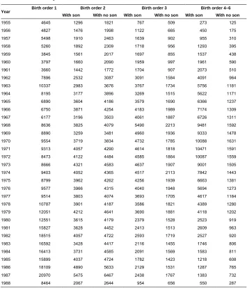
Table A-1: Sample size of birth records by birth order and sibship sex composition
Year Birth order 1 Birth order 2 Birth order 3 Birth order 4–6 With son With no son With son With no son With son With no son 1955 4645 1296 1821 767 509 273 125 1956 4827 1476 1998 1122 665 450 175 1957 5498 1910 2463 1639 902 955 310 1958 5260 1892 2309 1718 956 1293 395 1959 3845 1561 2017 1697 855 1537 438 1960 3797 1660 2090 1959 997 1961 590 1961 3660 1442 1772 1704 907 2073 510 1962 7896 2532 3087 3091 1584 4091 964 1963 10337 2983 3676 3767 1734 5756 1181 1964 8195 3177 3896 3269 1515 5622 1171 1965 6890 3604 4186 3579 1690 6366 1237 1966 6750 3871 4254 4183 1989 7174 1309 1967 6177 3196 3503 4061 1887 6726 1311 1968 8636 3825 4079 5490 2213 9481 1592 1969 8890 3259 3481 4960 1936 9333 1478 1970 9554 3719 3834 4732 1785 10088 1631 1971 9313 4057 4290 4614 1818 10471 1591 1972 8473 4122 4484 4585 1864 10087 1559 1973 8666 4321 4583 4637 1907 9001 1505 1974 9403 4052 4365 4517 2113 7842 1443 1975 8799 3962 4262 4256 1939 6663 1381 1976 9577 3966 4315 4040 1948 5694 1273 1977 9514 3803 4074 3693 1705 4617 1184 1978 10787 3901 4187 3586 1821 4389 1280 1979 12051 4212 4641 3690 1881 4118 1202 1980 12551 3615 4179 2379 1528 2523 919 1981 15827 3628 4452 2413 1513 2609 963 1982 18515 4057 4722 2593 1719 2527 920 1983 16592 3428 4417 2116 1455 1746 806 1984 16413 3731 4585 2091 1569 1583 811 1985 15899 4037 4724 1782 1423 1218 608 1986 18109 4890 5633 2129 1531 1287 765 1987 20970 5475 6467 2438 1767 1383 732 1988 8464 2067 2644 954 656 550 287
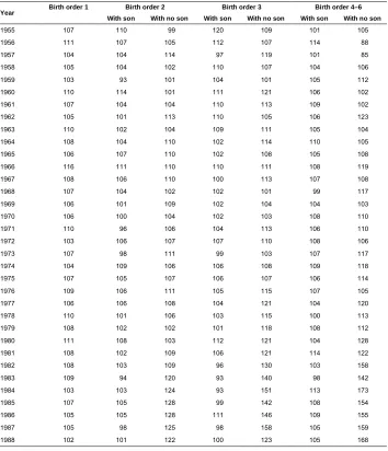
Table A-2: Unadjusted sex ratios by birth order and sibship sex composition
Year Birth order 1 Birth order 2 Birth order 3 Birth order 4–6 With son With no son With son With no son With son With no son 1955 107 110 99 120 109 101 105 1956 111 107 105 112 107 114 88 1957 104 104 114 97 119 101 85 1958 105 104 102 110 107 104 106 1959 103 93 101 104 101 105 112 1960 110 114 101 111 121 106 102 1961 107 104 104 110 113 109 102 1962 105 101 113 110 105 106 123 1963 110 102 104 109 111 105 104 1964 108 104 110 102 114 110 105 1965 106 107 110 102 108 105 108 1966 116 111 110 110 111 108 119 1967 108 106 110 100 113 107 108 1968 107 104 102 102 101 99 117 1969 106 101 109 102 104 104 103 1970 106 100 104 102 103 108 110 1971 110 96 106 104 113 106 110 1972 103 106 107 107 110 108 106 1973 107 98 111 99 103 107 117 1974 104 109 106 106 108 109 118 1975 107 105 107 106 107 106 114 1976 109 106 111 105 115 107 105 1977 106 106 108 104 121 104 120 1978 110 101 106 103 115 100 113 1979 108 102 102 101 118 108 112 1980 111 108 103 112 121 104 128 1981 108 102 109 106 121 114 122 1982 108 103 109 96 130 103 158 1983 109 94 120 93 140 98 142 1984 103 103 124 93 151 113 173 1985 107 105 128 99 142 108 154 1986 105 105 128 111 146 109 155 1987 105 98 125 98 158 105 159 1988 102 101 122 100 123 105 168
Table A-3: Marginal probability of a male birth, conditional on live birth; Rural and semi-rural subsample
First birth Second birth Third birth Birth year With
surviving son
Without surviving son
With surviving son
Without surviving son
With surviving son
Without surviving son 1965 –0.22% 0.32% 1.05% 0.21% 0.02% 1966 2.39% ** 2.27% ** 1.02% 1.50% ** 2.76% *** 1967 Reference year
1968 –0.58% –0.27% –0.94% –0.65% 0.65% 1969 –0.21% –0.48% 0.88% 0.21% –0.22% 1970 0.37% –1.23% 0.08% 0.86% 0.96% 1971 0.99% –1.91% 0.49% 0.48% 2.09% * 1972 –0.76% 12.29% 1.11% 1.24% * 1.60% 1973 0.23% –1.70% 1.58% 0.45% 1.33% 1974 –0.51% 1.26% 0.52% 1.33% * 2.31% ** 1975 0.25% –0.13% 0.75% 0.72% 1.76% ** 1976 1.59% 1.40% 2.70% * 0.95% 2.04% 1977 0.57% 2.68% * 1.51% 0.79% 4.94% *** 1978 1.80% –1.37% 0.46% 0.76% 3.10% ** 1979 0.45% 1.48% 42.36% 1.80% * 3.58% ** 1980 1.82% 4.42% ** –0.45% 1.49% 5.19% *** 1981 1.28% 1.16% 3.27% 2.44% 4.15% ** 1982 1.18% 4.52% *** 3.44% 0.01% 6.69%
Note: Each cell contains marginal probability that a birth occurring in each year, birth order, and sibling sex composition category is male. Marginal probabilities are calculated from coefficients estimated using OLS linear regressions (estimated separately for births of each order) of an indicator for a male birth on indicators for birth year and the sex composition of older siblings, as well as all two -way interactions between birth year and sibship sex composition. We control for residence in urban area, mother's educational attainment strata, mother's age at marriage, and time-invariant province fixed effects. Huber–White robust standard errors are clustered at the province level. * p<0.10, ** p<0.05, *** p<0.001.
Table A-4: Marginal probability of a male birth, conditional and live birth; rural subsample
First birth Second birth Third birth Birth year With
surviving son
Without surviving son
With surviving son
Without surviving son
With surviving son
Without surviving son 1965 –0.98% 0.69% 0.54% 0.04% –0.04% 1966 2.28% ** 3.11% ** 2.20% 1.79% * 2.53% ** 1967 Reference year
1968 –1.44% –0.26% –0.81% –0.88% 1.33% 1969 –0.40% 0.60% 0.68% 0.36% –0.34% 1970 0.32% –1.39% –0.19% 0.61% 1.76% * 1971 0.31% –1.62% 1.06% 0.47% 2.44% 1972 –1.22% –0.81% 2.14% 0.90% 1.59% 1973 –0.66% –1.93% 1.85% 0.39% 1.11% 1974 –0.99% 1.27% 0.24% 1.39% * 3.48% ** 1975 –1.02% –0.01% 0.99% 0.89% 2.61% *** 1976 1.01% 0.73% 3.65% ** 1.36% 2.73% * 1977 –0.77% 1.96% * 1.90% 1.16% 5.92% *** 1978 0.80% –2.67% 0.90% 0.65% 4.73% *** 1979 –0.43% 1.46% 0.47% 1.89% * 5.55% ** 1980 0.88% 4.80% ** 1.24% 0.54% 4.99% *** 1981 –0.21% –0.61% 3.41% 2.88% 5.38% ** 1982 –0.15% –1.06% 7.44% *** 4.76% ** 7.37%
Note: Each cell contains marginal probability that a birth occurring in each year, birth order, and sibling sex composition category is male. Marginal probabilities are calculated from coefficients estimated using OLS linear regressions (estimated separately for births of each order) of an indicator for a male birth on indicators for birth year and the sex composition of older siblings, as well as all two -way interactions between birth year and sibship sex composition. We control for residence in urban area, mother’s educational attainment strata, mother’s age at marriage, and time-invariant province fixed effects. Huber–White robust standard errors are clustered at the province level. * p<0.10, ** p<0.05, *** p<0.001.
Table A-5: Marginal probability of a male birth relative among third parity births with no previously born son
Full sample Rural + semirural subsample Rural subsample LPM Probit LPM Probit LPM Probit No Son x Parity 3 x Year = 1965 –0.01386 –0.03480 –0.01820 –0.04567 –0.01257 –0.03153
(0.013) (0.033) (0.014) (0.035) (0.015) (0.037) No Son x Parity 3 x Year = 1966 –0.00403 –0.01008 –0.00377 –0.00943 –0.00430 –0.01077
(0.015) (0.037) (0.015) (0.039) (0.019) (0.047) No Son x Parity 3 x Year = 1967 Reference year
No Son x Parity 3 x Year = 1968 –0.00493 –0.01241 –0.00330 –0.00829 0.01045 0.02620 (0.014) (0.036) (0.015) (0.037) (0.016) (0.040) No Son x Parity 3 x Year = 1969 –0.01924 –0.04830 –0.02065 –0.05182 –0.01873 –0.04697
(0.019) (0.046) (0.018) (0.046) (0.018) (0.045) No Son x Parity 3 x Year = 1970 –0.01699 –0.04266 –0.01533 –0.03847 –0.00023 –0.00058
(0.014) (0.035) (0.016) (0.039) (0.018) (0.044) No Son x Parity 3 x Year = 1971 –0.00416 –0.01043 –0.00023 –0.00057 0.00804 0.02022
(0.018) (0.045) (0.018) (0.044) (0.020) (0.050) No Son x Parity 3 x Year = 1972 –0.01873 –0.04700 –0.01272 –0.03190 –0.00474 –0.01186
(0.016) (0.041) (0.017) (0.041) (0.017) (0.044) No Son x Parity 3 x Year = 1973 –0.00821 –0.02064 –0.00752 –0.01887 –0.00456 –0.01145
(0.015) (0.037) (0.015) (0.038) (0.017) (0.044) No Son x Parity 3 x Year = 1974 –0.01006 –0.02524 –0.00649 –0.01628 0.00915 0.02304
(0.016) (0.041) (0.016) (0.040) (0.017) (0.044) No Son x Parity 3 x Year = 1975 –0.00817 –0.02050 –0.00596 –0.01495 0.00548 0.01379
(0.016) (0.041) (0.017) (0.044) (0.018) (0.045) No Son x Parity 3 x Year = 1976 –0.00787 –0.01977 –0.00544 –0.01365 0.00193 0.00487
(0.011) (0.027) (0.011) (0.027) (0.016) (0.039) No Son x Parity 3 x Year = 1977 0.02415 0.06092 0.02518 0.06351 0.03592* 0.09060*
(0.017) (0.042) (0.018) (0.045) (0.019) (0.048) No Son x Parity 3 x Year = 1978 0.00120 0.00302 0.00713 0.01796 0.02911 0.07328
(0.021) (0.052) (0.021) (0.053) (0.018) (0.045) No Son x Parity 3 x Year = 1979 –0.00076 –0.00183 0.00144 0.00369 0.02485 0.06267
(0.018) (0.044) (0.018) (0.045) (0.029) (0.073) No Son x Parity 3 x Year = 1980 0.01450 0.03666 0.02068 0.05218 0.03279 0.08248
(0.024) (0.061) (0.025) (0.062) (0.025) (0.064) No Son x Parity 3 x Year = 1981 0.00460 0.01172 0.00081 0.00213 0.01332 0.03366
(0.024) (0.061) (0.025) (0.063) (0.030) (0.075) No Son x Parity 3 x Year = 1982 0.04515* 0.11397* 0.05045* 0.12734* 0.01435 0.03679
(0.025) (0.063) (0.026) (0.065) (0.054) (0.138)
Note: Each cell contains marginal probability that a third- or higher-order birth occurring in each year to a couple with no previously born sons is male, relative to comparable births in the reference year 1969. Marginal probabilities are coefficients estimated using OLS linear regression or probit regression (as specified in column headers) of an indicator for birth year and the sex composition of older siblings, as well as all two-way interactions between birth year and sibship sex composition, estimated among third births. We control for residence in urban area, mother’s educational attainment strata, mother’s age at marriage, and time-invariant province fixed effects. Huber–White robust standard errors are clustered at the province level. * p<0.10, ** p<0.05, *** p<0.001.
Table A-6: Sex ratios at birth for all births, 1988 “Two-per-thousand” survey, 1990
1988 “Two-per-thousand”
survey
1990 Census Not adjusted for
mortality
Adjusted for mortality using:
Year 1988 Survey Coale 1984 Banister 1994 Jiang et al. 1984 1974 106.72 105.24 105.75 104.97 108.07 106.02 1975 106.25 105.74 106.03 105.54 108.67 106.53 1976 107.28 106.19 106.66 105.94 109.11 106.86 1977 107.02 106.49 106.66 106.17 109.37 107.03 1978 106.05 106.45 107.03 106.10 109.29 106.92 1979 105.77 106.84 107.19 106.45 109.64 107.23 1980 108.58 107.43 107.49 107.00 110.19 107.74 1981 107.83 107.37 107.52 107.02 110.19 107.71 1982 107.89 107.77 107.67 108.42 108.42 108.42 1983 108.28 108.69 108.90 109.31 109.31 109.31 1984 108.37 108.64 108.86 109.24 109.24 109.24 1985 110.87 108.65 108.88 109.22 109.22 109.22
1988 “Two-per-thousand”
survey
1982 Census Not adjusted for
mortality
Adjusted for mortality using:
Year 1988 Survey Coale 1984 Banister 1994 Jiang et al. 1984 1974 106.72 106.12 106.49 99.85 98.67 102.34 1975 106.25 106.18 106.43 105.26 107.03 106.24 1976 107.28 106.31 106.81 105.44 107.14 106.36 1977 107.02 106.27 106.43 105.44 107.08 106.29 1978 106.05 106.19 106.67 105.45 107.06 106.26 1979 105.77 106.71 107.14 106.05 107.64 106.83 1980 108.58 107.35 107.47 106.78 108.35 107.52 1981 107.83 107.83 108.17 107.34 108.89 108.04
Table A-7: Sex ratios at birth for second and third order births with no older male sibling
Second births with no older male sibling Third births with no older male sibling 1988
“two-per-thousand” survey
1990 Census 1988 “two-per-thousand”
survey
1990 Census Not adjusted
for mortality
Using survey-based mortality
Not adjusted for mortality
Using survey-based mortality Year
1977 107.54 106.82 105.69 120.87 116.00 114.21 1978 106.46 111.11 112.11 114.01 116.94 117.24 1979 102.31 111.41 111.10 115.59 122.17 120.45 1980 102.96 112.26 113.84 123.67 135.63 134.84 1981 108.62 114.92 114.46 121.67 135.93 131.88 1982 108.66 119.92 117.99 139.26 145.91 142.26 1983 120.19 128.13 125.21 140.53 162.85 154.30 1984 123.66 130.11 129.54 158.41 160.76 158.71 1985 127.88 128.52 128.55 145.29 160.54 156.53
Appendix 2: A simple conceptual framework for fertility decline and
sex selection
We formalize the intuition that as family size decreases, male-biased sex ratios increase. Our framework is adapted from Lin, Liu, and Qian (2014), who study the joint effect of legalized abortion and son preference on sex ratios at birth and relative female infant mortality rates in Taiwan. An important distinction is that the cost of sex selection in our model is an ex-post cost experienced through neglect; in contrast, most models treat this cost as an ex-ante cost (the cost of ultrasound, for example) (Anukriti 2016; Ebenstein 2011; Lin, Liu, and Qian 2014).
First, define the household utility function from giving births as:
– , (1)
where captures the utility of the child and varies with the child’s gender. Specifically, if a son is born, then = 1 + ; if a girl is born, then = 1. > 0 therefore captures the strength of son preference. > 0 is a cost parameter for raising children and can broadly be interpreted to include physical, financial, social, and psychological costs. Finally, without loss of generality, we assume households to have a reservation utility of zero from no children.
After a child is born, families can choose to neglect a child, which results in the child’s death, with cost c > 0. This cost of neglect c broadly reflects the physical, financial, social, and psychological burden of neglect. Households with sufficiently high opportunity cost > 1 + max ( − , ) will never have any children. Likewise, households with sufficiently low opportunity cost < 1 + min ( , ) will always become pregnant and not neglect. The remaining case includes families with intermediate values of , who become pregnant because of the option value of neglecting daughters:
1 + min ( , ) < < 1 + max − , . (2)
Once a daughter is born, households will prefer neglect to raising the daughter when:37
1 − < − . (3)
37 In our framework, a son is never neglected because households with such preferences would never initiate a
Inspection of Equation 2 makes clear that as increases, a family’s utility from having a daughter decreases – and hence the probability of neglect rises. Figure 2 shows these cases graphically.
In summary, as the cost of children increases, more families will choose to have no children, and some families that would otherwise become pregnant without neglect will now become pregnant – but instead neglect their daughters. In the aggregate, the impact on sex ratios is unambiguous: an increase in the cost of children (whatever the cause) leads not only to smaller family sizes, but also increased neglect of daughters and hence rising sex ratios.
Figure A-5: Graphical illustration of sex selection by strength of son preference and cost of raising a child