Volume 57, 2018, Pages 471–487
LPAR-22. 22nd International Conference on Logic for Programming, Artificial Intelligence and Reasoning
Improving SAT-based Bounded Model Checking for
Existential CTL through Path Reuse
Chuan Jiang and Gianfranco Ciardo
Department of Computer Science, Iowa State University Ames, Iowa, USA
{cjiang, ciardo}@iastate.edu
Abstract
A complementary technique to decision-diagram-based model checking is SAT-based bounded model checking (BMC), which reduces the model checking problem to a propo-sitional satisfiability problem so that the corresponding formula is satisfiable iff a coun-terexample or witness exists. Due to the branching time nature of computation tree logic (CTL), BMC for the universal fragment of CTL (ACTL) considers a counterexample in a bounded model as a set of bounded paths. Since the existential fragment of CTL (ECTL) is dual to ACTL, and ACTL formulas are often negated to obtain ECTL ones in practice, we focus on BMC for ECTL and propose an improved translation that generates a possibly smaller propositional formula by reducing the number of bounded paths to be considered in a witness. Experimental results show that the formulas generated by our approach are often easier for a SAT solver to answer. In addition, we propose a simple modification to the translation so that it is also defined for models with deadlock states.
1
Introduction
SAT-based bounded model checking (BMC) is a complementary technique to decision-diagram-based model checking [5]. By exploiting the observation that many real-life models have “shal-low” counterexamples or witnesses, BMC only considers finite prefixes of infinite paths. It translates the semantics of temporal logic, bounded by some integerk, into a propositional for-mula, and leverages a SAT solver to check for satisfiability. If the formula is determined to be satisfiable, a counterexample or witness can be generated from the truth assignment produced by the SAT solver. Otherwise, k is increased progressively until either a counterexample or witness is found, or some preset upper bound is reached. BMC was first proposed for linear temporal logic (LTL) [1, 2] and later applied to the universal fragment of computation tree logic (ACTL) [15] and∀µ-calculus [14,19]. Decision-diagram-based techniques inspired by the same idea were also proposed [18,21].
tree-like [9]. In [6, 15, 22], a counterexample or witness in a bounded model is represented as a set of bounded paths. Different encoding schemes based on proof system were proposed in [14, 19], in the larger context of ∀µ-calculus. In this paper, we improve the translation to propositional formulas from [6,15,22] by reducing the number of bounded paths that must be considered. Our approach generates a smaller formula, which is often easier for a SAT solver to answer, or the same one as in the classic approach, in the worst case. In addition, we propose a simple modification to the translation so that it is also defined for models with deadlock states. The remainder of this paper is organized as follows. Section2defines ECTL and its bounded semantics, and presents the translation of bounded semantics into a propositional formula. Section3proposes an improved translation to produce a possibly smaller propositional formula. Section4 compares the classic approach and ours with respect to the minimum bound to find a witness, which determines the earliest possibility for BMC to provide an answer, and with respect to the complexity of propositional formulas, in terms of the number of symbolic states considered to form a witness. Section5modifies the translation to cope with models containing deadlock states. Section6 describes our experimental design and presents the results, while Section7concludes our discussion and outlines future work.
2
Background
We denote sets by calligraphic letters (e.g.,A), except for the natural numbers N={0,1, ...}.
2.1
Kripke Structures and ECTL
A model is represented as a Kripke structure M = (S,Sinit,N,A,L), where S is the state
space,Sinit⊆ Sis the set of initial states,N ⊆ S × S is the total transition relation,Ais a set
of atomic propositions, andL:S →2Ais a labeling function that gives the atomic propositions holding in each state (subject totrue ∈ Aholding in every state). LetP be the set of paths in M, i.e., infinite sequences (s0, s1, ...) of states, where (si, si+1)∈ N for any i∈N.
We consider ECTL, the existential fragment of the temporal logic CTL [8], where formulas have the following syntax (ϕandρare ECTL formulas,ais an atomic proposition):
ϕ::=a| ¬a|ϕ∧ρ|ϕ∨ρ|EXϕ|E(ϕUρ)|EGϕ,
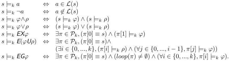
and the conditions for statesin model M to satisfy formulaϕ, written s|=ϕ(M is omitted for brevity), are as follows:
s|=a ⇔ a∈ L(s) s|=¬a ⇔ a6∈ L(s)
s|=ϕ∧ρ ⇔ (s|=ϕ)∧(s|=ρ) s|=ϕ∨ρ ⇔ (s|=ϕ)∨(s|=ρ)
s|=EXϕ ⇔ ∃(s0, s1, ...)∈ P,(s0≡s)∧(s1|=ϕ)
s|=E(ϕUρ) ⇔ ∃(s0, s1, ..., si, ...)∈ P,(s0≡s)∧(si|=ρ)∧(∀j∈ {0, ..., i−1}, sj |=ϕ)
s|=EGϕ ⇔ ∃(s0, s1, ...)∈ P,(s0≡s)∧(∀i∈N, si|=ϕ)
(formulasEFϕandE(ϕRρ) can be expressed asE(trueUϕ) andEGρ∨E(ρU(ϕ∧ρ)), respectively, so we do not discuss them separately).
Definition 2.1. An ECTL formulaϕis (existentially) valid in a modelM = (S,Sinit,N,A,L),
ACTL, the universal fragment of CTL, is the dual of ECTL. A counterexample to AXϕ,
AGϕ, orA(ϕUρ) is a witness for EX(¬ϕ),EF(¬ϕ), or E(¬ρU(¬ϕ∧ ¬ρ))∨EG(¬ρ), respectively (where the negation ¬ can be recursively “pushed down” to atomic propositions), i.e., the negation of an ACTL formula is an ECTL formula.
2.2
Bounded Semantics of ECTL
Given a modelM = (S,Sinit,N,A,L) andk∈ N, a k-path, or a path of length k, is a finite
sequence π = (s0, ..., sk) of k+ 1 states such that (si, si+1) ∈ N for any i ∈ {0, ..., k−1}.
Letπ[i] denotesi, the i-th state in π. A k-path, though finite, can still represent an infinite
path if the last state is the same as any of the previous states. We define a functionloop(π) to determine if ak-pathπis a loop:
loop(π) ={i∈ {0, ..., k−1} |π[k]≡π[i]},
thusloop(π)6=∅iffπis a loop.
In our definition, a loop is thus ak-path containing at least two states [12]. This is slightly different from the notation in [2, 15], which explicitly requires a back loop from the last state to some state on the path: {i∈ {0, ..., k} |(π[k], π[i])∈ N }. Figure1illustrates the two ways of thinking about, and defining, the same loop. We choose this notation because encoding state equivalence is often simpler and more compact than encoding a transition relation step. Our notation requiresk≥1, which we then assume in the rest of the paper.
s0 s1 s2 s3
(a) The loop shape in [2,15]
s0 s1 s2 s3 s4 s4≡s1
(b) The loop shape in this paper
Figure 1: The two kinds of loop shapes
Thek-model ofM is a tupleMk = (S,Sinit,Pk,A,L), wherePkis the set of all thek-paths
inM. The bounded semantics is defined over a k-modelMk.
Definition 2.2(Bounded semantics of ECTL). LetMk be thek-model of a modelM,sa state
ofM,aan atomic proposition, andϕ,ρECTL formulas. The conditions forsinMk to satisfy
ϕ, writtens|=k ϕ(Mk is omitted for brevity), are defined as follows:
s|=ka ⇔ a∈ L(s)
s|=k¬a ⇔ a6∈ L(s)
s|=kϕ∧ρ ⇔ (s|=kϕ)∧(s|=kρ)
s|=kϕ∨ρ ⇔ (s|=kϕ)∨(s|=kρ)
s|=kEXϕ ⇔ ∃π∈ Pk,(π[0]≡s)∧(π[1]|=k ϕ)
s|=kE(ϕUρ) ⇔ ∃π∈ Pk,(π[0]≡s)∧
(∃i∈ {0, ..., k},(π[i]|=kρ)∧(∀j ∈ {0, ..., i−1}, π[j]|=k ϕ))
s|=kEGϕ ⇔ ∃π∈ Pk,(π[0]≡s)∧(loop(π)6=∅)∧(∀i∈ {0, ..., k}, π[i]|=kϕ).
Theorem 2.1. Let M be a model, R the reachable states of M, s a state of M, and ϕ an ECTL formula. Then,s|=ϕiffs|=k ϕfor somek∈ {1, ...,|R|}.
Definition 2.3. An ECTL formulaϕis (existentially) valid in ak-modelMk= (S,Sinit,Pk,A,L),
Theorem 2.2. Given an ECTL formula ϕ,M |=ϕiffM |=kϕ for somek∈ {1, ...,|R|}.
Based on Theorem 2.2, an ECTL model checking problem is reduced to an ECTL BMC problem: the unbounded and bounded semantics are equivalent for a sufficiently large bound.
2.3
Translation into a Propositional Formula
SAT-based BMC for ACTL formulas was proposed in [15], and later improved with a more efficient translation to propositional formulas [6, 22]. Since it begins with negating an ACTL formula, this approach actually checks an ECTL formula over a bounded model. Compared to the original BMC for LTL [2], the main difference is that this approach represents a witness or counterexample as a set of symbolick-paths, due to the branching time nature of CTL. For example, a witness forEG(EFa) contains a lasso-shaped loop of length k where EFa holds in every state, and, for each state on that loop, a path of length k showing that we can reach a state satisfyinga from it. The boundk does not describe the size of a potential witness or counterexample, but the length of each individual path demonstrating satisfaction or violation of a subformula in a state.
The number ofk-paths needed to check an ECTL formula is given by a functionfk:
Definition 2.4. Function fk :ECT L→Nis defined as follows:
fk(a) = 0, wherea∈ A
fk(¬a) = 0, wherea∈ A
fk(ϕ∧ρ) = fk(ϕ) +fk(ρ)
fk(ϕ∨ρ) = max(fk(ϕ), fk(ρ))
fk(EXϕ) = fk(ϕ) + 1
fk(E(ϕUρ)) = k·fk(ϕ) +fk(ρ) + 1
fk(EGϕ) = k·fk(ϕ) + 1,
wherefk(EGϕ) is slightly different from that in [6,15,22] because of our loop notation.
For example, given a boundk, the maximum witness to show E(ϕUρ) consists of a k-path (s0, s1, ..., sk),fk(ρ)k-paths to showsk |=ρ, and, for eachi∈ {0, ..., k−1},fk(ϕ) k-paths to
showsi|=ϕ.
Symbolically, a state is represented as a vector of boolean variables. Let πi denote thei-th
symbolic k-path, which is a sequence of k+ 1 symbolic states. Checking an ECTL formula ϕ over a bounded model Mk is then reduced to checking the satisfiability of a propositional
formula [M, ϕ]k= [Mk]ϕ∧[ϕ]k, where:
• [Mk]ϕis a propositional formula that enforces thefk(ϕ) state sequences to be validk-paths
andπ0[0] to be an initial state:
[Mk]ϕ=I(π0[0])∧
fk(ϕ)−1 ^
i=0
k−1
^
j=0
N(πi[j], πi[j+ 1]),
whereI(s) iffs∈ Sinit andN(s, s0) iff (s, s0)∈ N.
• [ϕ]k = [ϕ, π0[0]]0k is a propositional formula that assembles k-paths and enforces ϕ or
subformulas ofϕon each correspondingk-path; specifically, [ϕ, s]i
k-path, where the first state of that k-path must be equivalent tos (unless ϕis a pure propositional formula):
[a, s]i
k = a(s), wherea∈ A
[¬a, s]ik = ¬a(s), wherea∈ A
[ϕ∧ρ, s]ik = [ϕ, s]ik∧[ρ, s]i+fk(ϕ)
k
[ϕ∨ρ, s]ik = [ϕ, s]ik∨[ρ, s]ik [EXϕ, s]i
k = (s≡πi[0])∧[ϕ, πi[1]]ik+1
[E(ϕUρ), s]i
k = (s≡πi[0])∧Wkj=0
[ρ, πi[j]]ik+1∧Vjt=0−1[ϕ, πi[t]]
i+1+fk(ρ)+t·fk(ϕ)
k
[EGϕ, s]i
k = (s≡πi[0])∧W
k−1
j=0(πi[k]≡πi[j])∧V k−1
j=0[ϕ, πi[j]]
i+1+j·fk(ϕ)
k ,
where, again, [EGϕ, s]ik is slightly different from that in [6,15,22].
For example, the interpretation of [E(ϕUρ), s]i
k is as follows: First, the first state of πi is
equivalent to the given states. Then, for each j ∈ {0, ..., k}, we start fromπi+1 to search for
a witness forρinπi[j], consisting offk(ρ)k-paths, and fromπi+1+fk(ρ)+t·fk(ϕ)to search for a witness forϕinπi[t], consisting of fk(ϕ)k-paths, for eacht∈ {0, ..., j−1}.
We refer to the translation above as the Classicapproach.
Theorem 2.3. Let M be a model, andϕan ECTL formula. M |=kϕiff[M, ϕ]k is satisfiable.
Theorem 2.4. M |=ϕiff for somek∈ {1, ...,|R|},[M, ϕ]k is satisfiable.
In practice, it is often the case that, if M |=ϕ, there exists a smallk such thatM |=k ϕ,
i.e., a “shallow” witness exists. This is the reason why BMC is often very efficient in error detection. The deeper the witness is, the less advantage BMC has.
3
Improved Translation of Bounded Semantics
We now give an example to explain how we improve onClassic. Given an ECTL formula, the goal of BMC is to find a witness demonstrating satisfaction. Figure2(a)can be viewed as a witness forEG(EFa) when k= 3, consisting of twok-paths, (1,2,3,2) and (3,4,5,∗), where
∗ can be any valid state, because we can extract Figure 2(b) from it. By reusing paths, we can represent a witness in such a compact form. For example, the witness forEFain state 2 is built by concatenating state 2 to the witness forEFain state 3. BMC can benefit from this compact form, since the minimum k to find a witness is determined by the longest subpath (not counting ∗) in it. We can find the witness in Figure 2(a) whenk = 3, since the longest subpath is (1,2,3,2). Without reusing, we must havek= 4, since the longest subpath is now (1,2,3,4,5), the witness for EFa in state 1, and use five k-paths to find that witness (in a different form) as shown in Figure2(c): (1, 2, 3, 2, 3), (1, 2, 3, 4, 5), (2, 3, 4, 5,∗), (3, 4, 5,∗,
∗), and (2, 3, 4, 5,∗).
Given two statessands0 such that (s, s0)∈ N, ifE(ϕUρ) (orEGϕ) holds ins0, andϕholds
1 2 3 2
4
5
∗
a
(a)
1 2 3 2
4
5 2
3
4
5 3
4
5
a
a a
(b)
1 2 3 2 3
2
3
4
5 3
4
5
∗
4
5
∗
∗
3
4
5
∗
a
a
a a
(c)
Figure 2: Different forms of witnesses forEG(EFa).
We then define an auxiliary functionµ:ECT L→ECT Lproviding thesufficient predeces-sor formulato be enforced in “any previous state”:
Definition 3.1. Function µ:ECT L→ECT Lis defined as follows:
µ(a) = a, where a∈ A
µ(¬a) = ¬a, wherea∈ A
µ(ϕ∧ρ) = µ(ϕ)∧µ(ρ) µ(ϕ∨ρ) = ϕ∨ρ µ(EXϕ) = EXϕ µ(E(ϕUρ)) = ϕ∨ρ µ(EGϕ) = µ(ϕ).
Theorem 3.1. Let M = (S,Sinit,N,A,L)be a model,s,s0 states ofM such that(s, s0)∈ N,
andϕan ECTL formula. Ifs0|=ϕands|=µ(ϕ), thens|=ϕ.
Proof. We only need to prove correctness in the cases of conjunction,EU, andEG.
• Ifs0|=E(ϕUρ) ands|=ϕ∨ρ, thens|=E(ϕUρ):
Ifs|=ρ, it is trivial to see thats|=E(ϕUρ). Ifs|=ϕ, sinceshas a successors0|=E(ϕUρ), thens|=E(ϕUρ) by the definition ofEU.
The proof for conjunction and EG is based on induction on the structure of the ECTL formula. The basis is thatµ(a) =a, whose correctness is trivial.
• Ifs0|=ϕ∧ρands|=µ(ϕ)∧µ(ρ), thens|=ϕ∧ρ:
Assume that, ifs0 |=ϕands|=µ(ϕ) thens|=ϕ, and that, if s0|=ρands|=µ(ρ) then s|=ρ. By these assumptions, we haves|=ϕands|=ρ, thuss|=ϕ∧ρ.
• Ifs0|=EGϕand s|=µ(ϕ), thens|=EGϕ:
It is worthwhile to emphasize that Theorem 3.1 does not hold if we define µ(ϕ∨ρ) as µ(ϕ)∨µ(ρ). Consider the simple example whereϕ=EGa andρ=EGb, in Figure3. (EGa)∨
(EGb) does not hold ins, because (s, s0, s0), obtained through path reuse, is not a witness for (EGa)∨(EGb) ins, even thougha∨b holds insand (s0, s0) witnesses (EGa)∨(EGb) ins0.
s s0
a b
Figure 3: An example showing thatµ(ϕ∨ρ)6=µ(ϕ)∨µ(ρ).
According to Theorem 3.1, given a finite path (s0, ..., sn), to enforce an ECTL formulaϕ
in si for anyi∈ {0, ..., n}, we enforcesn |=ϕbut just si |=µ(ϕ), for i∈ {0, ..., n−1}, which
usually simplifies the formula to be enforced insi.
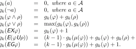
We define function gk, as an improvement of fk, giving the potentially smaller number of
k-paths needed to check an ECTL formula in a bounded model. gk differs fromfk only in the
case ofEU andEG:
Definition 3.2. Function gk :ECT L→Nis defined as follows:
gk(a) = 0, wherea∈ A
gk(¬a) = 0, wherea∈ A
gk(ϕ∧ρ) = gk(ϕ) +gk(ρ)
gk(ϕ∨ρ) = max(gk(ϕ), gk(ρ))
gk(EXϕ) = gk(ϕ) + 1
gk(E(ϕUρ)) = (k−1)·gk(µ(ϕ)) +gk(ϕ) +gk(ρ) + 1
gk(EGϕ) = (k−1)·gk(µ(ϕ)) +gk(ϕ) + 1.
For example, given a bound k, the maximum witness to show E(ϕUρ), according to our approach, consists of ak-path (s0, ..., sk),gk(ρ) k-paths to showsk |=ρ, gk(ϕ) paths to show
sk−1 |=ϕ, and, for each i∈ {0, ..., k−2}, gk(µ(ϕ))k-paths to show si |=µ(ϕ), since si |=ϕ
can be inferred.
Theorem 3.2. Given an ECTL formula ϕ,gk(µ(ϕ))≤gk(ϕ).
Theorem 3.3. Given an ECTL formula ϕ,gk(ϕ)≤fk(ϕ).
Then, we update the translation of conjunctive, EU, and EG formulas to propositional formulas (while we just replacefk withgk for the remaining formulas):
[ϕ∧ρ, s]i
k = [µ(ϕ), s] i
k∧[µ(ρ), s]
i+gk(µ(ϕ))
k
[E(ϕUρ), s]ik = (s≡πi[0])∧
[ρ, πi[0]]ik+1∨
Wk
j=1 [ρ, πi[j]]ik+1∧[ϕ, πi[j−1]]
i+1+gk(ρ)
k
∧Vj−2
t=0[µ(ϕ), πi[t]]
i+1+gk(ρ)+gk(ϕ)+t·gk(µ(ϕ))
k
[EGϕ, s]i
k = (s≡πi[0])∧Wjk=0−1(πi[k]≡πi[j])
∧[ϕ, πi[k−1]]ik+1∧
Vk−2
j=0[µ(ϕ), πi[j]]
i+1+gk(ϕ)+j·gk(µ(ϕ))
k .
We refer to this new translation as theReuseapproach.
propositional formula asClassic. For some ECTL formulas whose general form of witnesses is not linear (e.g.,EG(EXa), (EGa)∨(EGb)), the two approaches may also generate the same formulas. A complete template of ECTL formulas for whichgk(ϕ)< fk(ϕ) is still unclear.
4
Comparison of the Two Translation Approaches
In this section, we compareClassicandReuse with respect to the minimum bound needed to find a witness (Section4.1) and the complexity of propositional formulas (Section4.2).
4.1
Minimum Bound to Find a Witness
We already saw an example whereReusefinds a witness using a smallerkthanClassic, at the beginning of Section3. LetkClassic
min andkReusemin denote the minimum bounds for whichClassic
andReusefind a witness for a particular formula, respectively.
Theorem 4.1. Given an ECTL formula ϕholding in a modelM,kReuse
min ≤kClassicmin .
Proof. If Classicfinds a witness,Reusecan always find a witness in the compact form, as a substructure of the witness found by Classic, thus using the same k. For example, suppose
Classicfinds the witness forE((EFa)Ub) shown in Figure4(a), usingk= 3. Its substructure
(shown in the dashed box) is a witnessReusecan also find. This implies that kReuse
min is never
greater thankClassic
min .
Theorem 4.2. Given an ECTL formulaϕ holding in a model M,kClassic
min can be as large as
2kReuse
min −1.
Proof. To prove this theorem, it suffices to consider the ECTL formulaϕ=E(E(aUb)Uc) and the model shown in Figure4(b). Reuseseeks twok-paths, one pathπwhere someπ[j] satisfies c,π[j−1] satisfiesE(aUb), andπ[0], ..., π[j−2] satisfyµ(E(aUb)) =a∨b, and another pathσ whereσ[0] coincides withπ[j−1], someσ[l] satisfiesb, andσ[0], ..., σ[l−1] satisfya. For the model in Figure4(b), these two paths correspond to (s0, ..., sn−1, tc) and (sn−1, ..., s2n−2, tb),
respectively, andReusefinds them using a bound as low askReuse
min =n.
Instead, Classic seeks k+ 1 k-paths, the first one, π, where some π[j] satisfies c, and π[0], ..., π[j −1] satisfy E(aUb), as shown by the j k-paths σ0, ..., σj−1 having initial state
π[0], ..., π[j−1], respectively (the remaining k−j paths can be any valid k-paths). For the model in Figure4(b), pathπcorresponds to (s0, ..., sn−1, tc), the same as forReuse; however,
pathσ0 cannot be built unlessk≥2n−1, thuskminClassic= 2n−1.
4.2
Complexity of Propositional Formulas
We now compare the complexity of propositional formulas generated byClassicandReusein terms of the number of symbolic states needed to form a witness,NClassic(ϕ) = (k+ 1)·fk(ϕ)
andNReuse(ϕ) = (k+ 1)·gk(ϕ). Modern SAT solvers accept formulas in conjunctive normal
1 2 3 4
5
6
∗
7
∗
∗
8
9
10
a a
a b
(a) A witness forE((EFa)Ub)
s0 s1 ... sn−1 tc
sn
...
s2n−2
tb
a a a c
a
a
b
(b) A model whereE(E(aUb)Uc) holds
Figure 4: Examples used in the proofs of Theorem4.1and4.2.
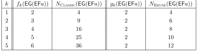
We first consider the simple formulaEG(EFa). Table1lists the values ofNClassic(EG(EFa)) and NReuse(EG(EFa)) w.r.t. k. It can be seen that NClassic(EG(EFa)) grows quadratically, whileNReuse(EG(EFa)) grows linearly, askincreases. The largerk is, the more significant the difference becomes.
k fk(EG(EFa)) NClassic(EG(EFa)) gk(EG(EFa)) NReuse(EG(EFa))
1 2 4 2 4
2 3 9 2 6
3 4 16 2 8
4 5 25 2 10
5 6 36 2 12
Table 1: Comparing the two translation approaches onEG(EFa): fk(EG(EFa)) =k·fk(EFa) + 1 =k·(fk(a) + 1) + 1 =k+ 1,
gk(EG(EFa)) = (k−1)·gk(µ(EFa)) +gk(EFa) + 1 = (k−1)·gk(a) + (gk(a) + 1) + 1 = 2.
Then, let us investigate a family of more complex formulas. Letai be an atomic proposition
for i ∈ N and consider the family of ECTL formulas {ϕ1, ϕ2, ...}, where ϕ1 =E(a0Ua1) and
ϕi=E(ϕi−1Uai) fori≥2. According to Def.2.4, fk(ϕ1) = 1 and, fori∈ {2, ..., n},
fk(ϕi) =k·fk(ϕi−1) + 1,
which can be rewritten as
fk(ϕi) +k−11
fk(ϕi−1) +k−11
=k .
This implies thatfk(ϕ1)+k−11, fk(ϕ2)+k−11, ..., fk(ϕi)+k−11 is a geometric series with ratiok.
Since its first elementfk(ϕ1) +k−11 equals 1 +k−11 = k−k1, itsi-th elementfk(ϕi) +k−11 equals ki
k−1, from which we can conclude that
fk(ϕi) =
ki−1
Finally,
NClassic(ϕi) = (k+ 1)·fk(ϕi) =
k+ 1 k−1(k
i−1). (1)
Now we compute NReuse(ϕi). According to Def. 3.2, gk(ϕ1) = 1, gk(ϕ2) = 2, and, for
i∈ {3, ..., n},
gk(ϕi) = (k−1)·gk(µ(ϕi−1)) +gk(ϕi−1) +gk(ai) + 1
= (k−1)·gk(ϕi−2∨ai−1) +gk(ϕi−1) + 1
= (k−1)·gk(ϕi−2) +gk(ϕi−1) + 1.
We build two geometric series by rewriting the equation above as
gk(ϕi)−1−
√
4k−3
2 gk(ϕi−1)− 2 1−√4k−3
gk(ϕi−1)−1−
√
4k−3
2 gk(ϕi−2)− 2 1−√4k−3
= 1 +
√
4k−3 2
and
gk(ϕi)−1+
√
4k−3
2 gk(ϕi−1)− 2 1+√4k−3
gk(ϕi−1)−1+
√
4k−3
2 gk(ϕi−2)− 2 1+√4k−3
=1−
√
4k−3
2 .
Therefore, the two geometric series have ratio 1+
√
4k−3
2 and
1−√4k−3
2 , respectively. Following
similar steps to those used to computefk(ϕi), we obtain
gk(ϕi)−
1−√4k−3
2 gk(ϕi−1)− 2
1−√4k−3 =−
1 +√4k−32 2 1−√4k−3·
1 +√4k−3 2
i−2
=− 2
1−√4k−3 ·
1 +√4k−3 2
i ,
gk(ϕi)−
1 +√4k−3
2 gk(ϕi−1)− 2
1 +√4k−3 =−
1−√4k−32 2 1 +√4k−3·
1−√4k−3 2
i−2
=− 2
1 +√4k−3 · 1
−√4k−3 2
i .
Combining the two equations above, we have:
gk(ϕi) =
1 +√4k−3i+2
− 1−√4k−3i+2 (k−1)·2i+2·√4k−3 −
1 k−1.
Finally,
NReuse(ϕi) = (k+ 1)·gk(ϕi) =
k+ 1 k−1
1 +√4k−3i+2− 1−√4k−3i+2 2i+2·√4k−3 −1
! . (2)
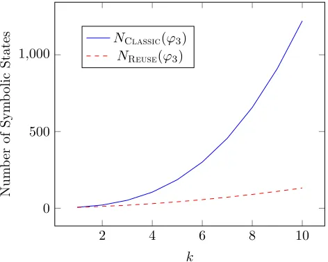
Note that i is a constant for a given formula in the family we are considering. Therefore, according to Equations1 and2, NClassic(ϕi)∼O(ki) andNReuse(ϕi)∼O(k
i+1
2 ). To visualize the difference between the two, we plot NClassic(ϕ3) and NReuse(ϕ3) in Figure 5. It can be
2 4 6 8 10 0
500 1,000
k
Num
b
er
of
Sym
b
ol
ic
States
NClassic(ϕ3)
NReuse(ϕ3)
Figure 5: Comparing the growth ofNClassic(ϕ3) andNReuse(ϕ3).
5
Coping with Models Containing Deadlock States
Generally, CTL assumes that the model does not contain any deadlock state. Unfortunately, this assumption is not true for many real-life models. For models containing deadlock states, using eitherClassicor Reusemay fail to find a witness if deadlock states are part of every witness. Figure6shows a simple model containing a deadlock state 4. Suppose we are searching a witness forEF(a∧EFb), which consists of twok-paths. There is no such witness whenk= 1, because we must take two steps from the initial state to reach a state wherea holds. When k= 2, the corresponding propositional formula is also unsatisfiable, because we are not able to build a path of length 2 from state 3.
1 2 3 4
a b
Figure 6: A model containing a deadlock state 4.
A common practice to cope with models containing deadlock states is to add a self-loop to every deadlock state. When using a SAT solver, we propose another approach that adds additional variables to the propositional formula, so that the formula allows k-paths whose actual length is smaller thank. Each symbolic stateπi[j] is associated with a boolean variable
τi,j, calledtransition flag, which istrue if and only ifπi[j] is a true successor of πi[j−1], i.e.,
N(πi[j−1], πi[j]). We modify the encoding of [Mk] as follows:
[Mk]ϕ=I(π0[0])∧
fk(ϕ)−1 ^
i=0
k−1
^
j=0
(N(πi[j], πi[j+ 1])∨τi,j+1)∧
fk(ϕ)−1 ^
i=0
k−1
^
j=0
(τi,j+1⇒τi,j).
The constraintN(πi[j], πi[j+ 1])∨τi,j+1 relaxes the assumption that πi[j] must have
suc-cessors, by simply setting τi,l to false for l ∈ {j+ 1, ..., k} if πi[j] is a deadlock state. The
constraint Vfk(ϕ)−1
i=0
Vk−1
symbolic stateπi[j+ 1] is reachable fromπi[0], i.e.,V j
l=0N(πi[l], πi[l+ 1]), otherwiseπi[j+ 1]
can take an arbitrary state.
The translation ofEX,EF, andEUformulas is also updated (we demonstrate the modification
toReuse; similar modification can also be applied toClassic):
[EXϕ, s]ik = (s≡πi[0])∧[ϕ, πi[1]]ik+1∧τi,1
[E(ϕUρ), s]i
k = (s≡πi[0])∧
[ρ, πi[0]]ik+1∧τi,0
∨Wk
j=1 [ρ, πi[j]]ik+1∧[ϕ, πi[j−1]]
i+1+gk(ρ)
k
∧Vj−2
t=0[µ(ϕ), πi[t]]
i+1+gk(ρ)+gk(ϕ)+t·gk(µ(ϕ))
k ∧τi,j
[EGϕ, s]ik = (s≡πi[0])∧W k−1
j=0(πi[k]≡πi[j])
∧[ϕ, πi[k−1]]ik+1∧V k−2
j=0[µ(ϕ), πi[j]]
i+1+gk(ϕ)+j·gk(µ(ϕ))
k ∧τi,k.
Of course, if the model is known to be deadlock-free (using a priori knowledge, or some deadlock detection technique), the proposed modification should not be applied, as it increases the size of the resulting formulas.
6
Experiments
We describe our experimental design in Section6.1and present the results in Section6.2.
6.1
Experimental Design
We implemented both Classic and Reusein the model checker SMART [7], making use of the SAT solver Nigma [10,11]. Our benchmark suite is a subset of models and CTL formulas from the CTL cardinality examination of the Model Checking Contest (MCC) 2018 (https: //mcc.lip6.fr/). Models are described as Petri nets, most of which have one or more scaling parameters, affecting size and complexity. An experimental instance is a pair of a model instance and an ECTL formula. To select a set of instances eligible for our experiment, we apply the following filtering process:
1. Run SMART up to 1 hour to determine if the model instance is a safe Petri net (the maximum number of tokens at each place is 1). Discard unsafe Petri nets, so that the places in the remaining model instances can be represented as binary variables (while the places in bounded unsafe Petri nets can be represented using one-hot or binary encoding, we restrict ourselves to safe Petri nets for convenience). In practice, we used the results published in MCC 2018. This leaves 2,256 instances.
10−1 100 101 102
10−1
100
101
102
Reuse
Classic
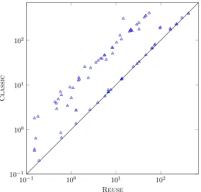
Figure 7: Comparing the total time (in seconds) spent on CNF transformation.
Finally, we have 89 instances, taken from 60 model instances from 22 different models. Among the 89 instances, the ECTL formulas hold in 50 instances, do not hold in 32 instances, while it is not known whether they hold in the remaining 7 instances, according to SMART.
To compare the performance of the two translation approaches, we run BMC up tok= 20. For eachk, the SAT solver is given 10 minutes to work on the generated CNF formula. BMC terminates either if a witness is found for somek, or if, for every k up to 20, the SAT solver reports UNSAT or runs out of time. In the latter case, we cannot conclude satisfaction or violation of the corresponding ECTL formula, but we can tell that there is no witness up to the largestkfor which the SAT solver reports UNSAT (no “simple” witness exists).
The model instances from MCC 2018 may contain deadlock states, thus we always apply the modification proposed in Section5.
6.2
Experimental Results
First, we compare the time spent on transforming propositional formulas into CNF. Since
Reusenever generates a larger propositional formula thanClassic, it is expected to
outper-form Classic on this metric, and the results confirm our expectation. Figure 7 presents a
10−1 100 101 102 103 104
10−1
100
101
102
103 104
2,0 0,2
9,9 13,12
13,6 16,16
0,1 2,21,1
10,0 6,1
7,0 9,9 9,9 10,10
Reuse
Classic
0.6 0.8 1
·104
0.6 0.8
1 ·10
4
9,9
13,12
13,6 16,16
9,9 9,9
10,10
Category 1 Category 2 Category 3 Category 4
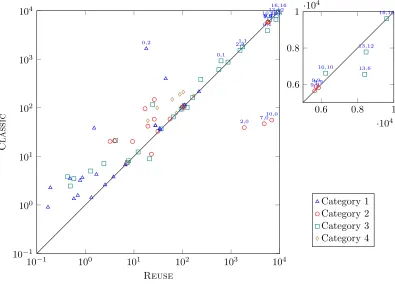
Figure 8: Comparing the total time (in seconds) spent on satisfiability checking.
Then, we compare the time spent on satisfiability checking. The results on each experimental instance are classified according to the following categories:
Category 1 (4) The ECTL formula holds, and at least one approach found a witness.
Category 2 () The ECTL formula holds, but neither approach found a witness.
Category 3 () The ECTL formula does not hold.
Category 4 (♦) We do not know whether the ECTL formula holds or not.
Figure 8 presents a logscale scatter plot comparing the total time (in seconds) spent on satisfiability checking. It also has a zoom-in view of the top-right corner in linear scale for clarity. A data point above the diagonal means that the SAT solver terminates (reporting SAT or UNSAT, or running out of time) in a shorter total time, working on the propositional formulas generated by Reuse. The pair of numbers i, j above a data point (omitted if 0,0) report the number of timeouts forReuseand Classic, respectively. For most instances, we can observe a better performance usingReuse.
Instances in Category 1 are those where we can take full advantage of BMC. For them,
Reusealways found a witness faster. There is even one instance (the topmost 4in Figure8)
Most instances in Category 2 have relatively “deep” witnesses. BMC may find a witness running with a largerk, at the risk of working on a huge and complex propositional formula. The rightmost three’s below the diagonal are instances where the SAT solver struggled with the formulas generated byReuse. We noticed more timeouts using Reusein these instances, which provides more evidence of the well-known fact that there is no strict connection between the size and the hardness of formulas for satisfiability checking [13].
In practice, BMC is not able to answer the instances in Category 3 and Category 4, since the upper bound of the maximal length of symbolic paths is the number of reachable states (see Theorem2.2), often a huge number. In these cases, BMC can only tell us that no “simple” witness exists (up to the largestkfor which the SAT solver reports UNSAT). We can see that most of the time,Reusedraws this conclusion faster thanClassic.
Finally, we select an experiment instance from Category 1 for a detailed comparison for each value ofk in Table 2. The model instance is AutoFlight-PT-05a and the formula is the negation of A((p33≤p79)U AG(p89≤p88)). BMC finds a witness fork = 17 using Classic and for k = 13 using Reuse. Vars, Clauses and Literals are the numbers of variables, clauses, and literals in the CNF formulas. We can see that the CNF formulas generated by
Reusegrow slower and are significantly smaller than the ones generated by Classic. CNF
and SAT are the time (in seconds) spent in CNF transformation and satisfiability checking, respectively. CNF transformation always benefits fromReuse, but satisfiability checking may not. WithReuse, the SAT solver spends more time reporting UNSAT fork= 8, 9, 10, 11, and 12, though this disadvantage is finally offset by reporting SAT and terminating for a smallerk. An explanation could be that for some model checking problems, a small CNF formula may also have a small unsatisfiable core, which can be deep and hard for a SAT solver to identify. For example, suppose that we are searching ak-pathπwhereπ[i]|=kEFafor anyi∈ {0, ..., k−1}.
For the formula generated byClassic, the SAT solver reports UNSAT as long as it finds ani such thatπ[i]6|=k EFa. However, for the formula generated by Reuse, it reports UNSAT only
when it proves thatπ[k−1]6|=k EFa.
In addition, the SAT solver reports SAT faster on a large formula (k = 17 for Classic; k= 13 forReuse) than it reports UNSAT on a small formula (k= 16 for Classic;k= 12 for
Reuse), which confirms that the hardness of satisfiable and unsatisfiable formulas should be
evaluated using different criteria.
7
Conclusions and Future Work
We have presented an improved translation to propositional formulas for ECTL BMC, which generates smaller, or at worst the same formulas as the ones generated by Classic. Exper-imental results show that CNF transformation always benefits from our approach, and that satisfiability checking is more efficient most of the time. In addition, we proposed a simple modification to the translation so that it is also defined for models containing deadlock states. BMC for ACTL formulas having linear counterexamples has been investigated in [20]. It seems promising to combine their work and ours, because our approach has advantages for formulas that are not instantiated from linear templates, thus the two approaches work on disjoint sets of ECTL and ACTL formulas and have no conflict in application.
k Classic Reuse
Vars Clauses Literals CNF SAT Vars Clauses Literals CNF SAT
1 2,357 27,108 56,460 0.04 0.00 2,357 27,108 56,460 0.04 0.00 2 5,384 70,968 147,217 0.12 0.02 4,172 53,661 111,547 0.08 0.01
3 9,353 131,733 272,576 0.23 0.06 5,985 80,213 166,632 0.13 0.02 4 14,266 209,405 432,541 0.41 0.06 7,798 106,766 221,719 0.18 0.03
5 20,123 303,984 627,112 0.59 0.09 9,611 133,320 276,808 0.25 0.05 6 26,924 415,470 856,289 0.82 0.15 11,424 159,875 331,899 0.28 0.06
7 34,669 543,863 1,120,072 1.18 0.22 13,237 186,431 386,992 0.35 0.22 8 43,358 689,163 1,418,461 1.53 0.27 15,050 212,988 442,087 0.4 0.61
9 52,991 851,370 1,751,456 1.68 0.32 16,863 239,546 497,184 0.45 1.67 10 63,568 1,030,484 2,119,057 2.20 0.39 18,676 266,105 552,283 0.52 2.76
11 75,089 1,226,505 2,521,264 2.91 1.64 20,489 292,665 607,384 0.59 5.04 12 87,554 1,439,433 2,958,077 3.03 2.61 22,302 319,226 662,487 0.61 28.66
13 100,963 1,669,268 3,429,496 3.67 2.30 24,115 345,788 717,592 0.64 5.95 14 115,316 1,916,010 3,935,521 4.00 28.05
15 130,613 2,179,659 4,476,152 5.10 27.50 16 146,854 2,460,215 5,051,389 5.28 220.14
17 164,039 2,757,678 5,661,232 6.02 112.17
Total 38.81 395.99 4.52 45.08
Table 2: Searching for a counterexample toA((p33≤p79)U AG(p89≤p88)) in AutoFlight-PT-05a.
Acknowledgments
This work was supported in part by the National Science Foundation under grant ACI-1642397.
References
[1] Armin Biere, Alessandro Cimatti, Edmund M Clarke, Ofer Strichman, and Yunshan Zhu. Bounded model checking. Advances in Computers, 58(11):117–148, 2003.
[2] Armin Biere, Alessandro Cimatti, Edmund M. Clarke, and Yunshan Zhu. Symbolic model checking without BDDs. InProc. TACAS, pages 193–207. Springer, 1999.
[3] Frederik Bønneland, Jakob Dyhr, Peter G Jensen, Mads Johannsen, and Jiˇr´ı Srba. Simplifica-tion of CTL formulae for efficient model checking of Petri nets. InInternational Conference on Applications and Theory of Petri Nets and Concurrency, pages 143–163. Springer, 2018.
[4] Francesco Buccafurri, Thomas Eiter, Georg Gottlob, and Nicola Leone. On ACTL formulas having linear counterexamples. Journal of Computer and System Sciences, 62(3):463–515, 2001.
[5] Jerry R Burch, Edmund M Clarke, Kenneth L McMillan, David L Dill, and Lain-Jinn Hwang. Symbolic model checking: 1020states and beyond. Information and Computation, 98(2):142–170, 1992.
[7] Gianfranco Ciardo, Robert L. Jones, Andrew S. Miner, and Radu Siminiceanu. Logical and stochastic modeling with SMART. Perf. Eval., 63:578–608, 2006.
[8] E. M. Clarke and E. A. Emerson. Design and synthesis of synchronization skeletons using branching time temporal logic. InProc. IBM Workshop on Logics of Programs, LNCS 131, pages 52–71, 1981. [9] Edmund M. Clarke, Somesh Jha, Yuan Lu, and Helmut Veith. Tree-like counterexamples in model
checking. InProc. LICS, pages 19–29. IEEE Comp. Soc. Press, 2002. [10] Chuan Jiang and Gianfranco Ciardo. Nigma 1.2. InSAT Race, 2015.
[11] Chuan Jiang and Ting Zhang. Partial backtracking in CDCL solvers. InInternational Conference on Logic for Programming Artificial Intelligence and Reasoning, pages 490–502. Springer, 2013. [12] Timo Latvala, Armin Biere, Keijo Heljanko, and Tommi Junttila. Simple bounded LTL model
checking. InInternational Conference on Formal Methods in Computer-Aided Design, pages 186– 200. Springer, 2004.
[13] Zolt´an ´Ad´am Mann. Typical-case complexity and the SAT competitions. In Daniel Le Berre, editor, POS-14. Fifth Pragmatics of SAT workshop, volume 27 of EPiC Series in Computing, pages 72–87. EasyChair, 2014.
[14] Rotem Oshman and Orna Grumberg. A new approach to bounded model checking for branching time logics. InInternational Symposium on Automated Technology for Verification and Analysis, pages 410–424. Springer, 2007.
[15] Wojciech Penczek, Bo˙zena Wo´zna, and Andrzej Zbrzezny. Bounded model checking for the uni-versal fragment of CTL. Fundamenta Informaticae, 51(1-2):135–156, 2002.
[16] David A Plaisted and Steven Greenbaum. A structure-preserving clause form translation.Journal of Symbolic Computation, 2(3):293–304, 1986.
[17] Grigori S Tseitin. On the complexity of derivation in propositional calculus. InAutomation of reasoning, pages 466–483. Springer, 1983.
[18] Andr´as V¨or¨os, D´aniel Darvas, and Tam´as Bartha. Bounded saturation-based CTL model checking. Proceedings of the Estonian Academy of Sciences, 62(1):59–70, 2013.
[19] Bow-Yaw Wang. Proving∀µ-calculus properties with SAT-based model checking. InInternational Conference on Formal Techniques for Networked and Distributed Systems, pages 113–127. Springer, 2005.
[20] Zhaowei Xu and Wenhui Zhang. Linear templates of ACTL formulas with an application to SAT-based verification.Information Processing Letters, 127:6–16, 2017.
[21] Andy Jinqing Yu, Gianfranco Ciardo, and Gerald L¨uttgen. Bounded reachability checking of asynchronous systems using decision diagrams. In Proc. TACAS, LNCS 4424, pages 648–663, 2007.