Int. J. IndustrialMathematics (ISSN 2008-5621)
Vol. 6, No. 1, 2014 Article ID IJIM-00410, 8 pages Research Article
Approximate solution of the stochastic Volterra integral equations via
expansion method
M. Khodabin ∗ † , K. Maleknejad ‡ , T. Damercheli §
————————————————————————————————–
Abstract
In this paper, we present an efficient method for determining the solution of the stochastic second kind Volterra integral equations (SVIE) by using the Taylor expansion method. This method transforms the SVIE to a linear stochastic ordinary differential equation which needs specified boundary conditions. For determining boundary conditions, we use the integration technique. This technique gives an approximate simple and closed form solution for the SVIE. Expectation of the approximating process is computed. Some numerical examples are used to illustrate the accuracy of the method.
Keywords: Taylor series expansion; Stochastic Volterra integral equation; Itˆo integral.
—————————————————————————————————–
1
Introduction
T
hin many applications such as mathemati-e stochastic Volterra integral equations arise cal finance, biology, medical, social sciences, etc. There is an increasing demand for studying the behavior of a number of sophisticated dynamical systems in physical, medical and social sciences, as well as in engineering and finance. These sys-tems are often dependent on a noise source, Gaus-sian white noise, for example, governed by cer-tain probability laws, so that modeling such phe-nomena naturally requires the use of various the∗Corresponding author. [email protected] †Department of Mathematics, Karaj Branch, Islamic Azad University, Karaj, Iran.
‡Department of Mathematics, Karaj Branch, Islamic Azad University, Karaj, Iran.
§Department of Mathematics, Karaj Branch, Islamic Azad University, Karaj, Iran.
stochastic differential equations and the stochas-tic optimization problem [1, 2, 4, 5, 6, 10] or, in more complicated cases, the stochastic Volterra integral equations and the stochastic integro-differential equations [3, 7, 12, 13, 15, 16, 17]. Since in many problems, such equations, can not be solved explicitly, it is important to find their approximate solutions by using some numerical methods. The methods for the computational so-lution of stochastic integral equations are based on similar techniques for deterministic integral equations, but generalized to provide support for stochastic dynamics [4, 5, 8, 9, 10, 11].
In this paper, a novel, simple, and an effi-cient approach is proposed to determine the ap-proximate solutions of the stochastic second kind Volterra integral equations. We use the Taylor series expansion of the unknown function for ob-taining the solution. Then for determining spec-ified boundary conditions, for transformed linear
ordinary differential equation, we employ the in-tegration method. This method is simple and effective, and can provide an accurate approxi-mate solution to the stochastic integral equations. The efficiently and the accuracy of the method are shown by some numerical examples from [11]. This paper is organized as follows: Section2, de-scribes the elementary concepts from stochastic calculus. In Section 3, we introduce the Taylor expansion method and exhibit the convergence of the proposed scheme in Section 4. The accuracy of the presented method is illustrated by some ex-amples in Section5. Finally, Section6gives some brief conclusions.
2
Stochastic Volterra integral
equations
We will begin with a quick survey of the most fun-damental concepts from stochastic calculus that are needed. For full details, the reader may consult Klebaner (1998), Oksendal (1998), Steele (2001).
A set of random variables Xt indexed by
real numbers t ≥ 0 is called a continuous-time stochastic process. Each instance, or realization of the stochastic process is a choice from the random variable Xt for each t, and is therefore
a function of t. Any (deterministic) function f(t) can be trivially considered as a stochastic process, with variance V(f(t)) = 0. An archety-pal example that is ubiquitous in models from physics, chemistry, and finance is the Wiener processWt, a continuous-time stochastic process
with the following three properties:
Property 1. For each t, the random variable Wt is normally distributed with mean 0 and
variancet.
Property 2. For each t1 < t2, the normal random variable Wt2-Wt1 is independent of the
random variable Wt1 , and in fact independent
of allWt,0≤t≤t1.
Property 3. The Wiener process Wt can be
represented by continuous paths where is not
differentiable.
The Wiener process, named after Norbert Wiener, is a mathematical construct that for-malizes random behavior characterized by the botanist Robert Brown in 1827, commonly called Brownian motion. It can be rigorously defined as the scaling limit of random walks as the step size and time interval between steps both go to zero. Brownian motion is crucial in the model-ing of stochastic processes since it represents the integral of idealized noise that is independent of frequency, called white noise. Often, the Wiener process is called upon to represent random, exter-nal influences on an otherwise deterministic sys-tem, or more generally, dynamics that for a va-riety of reasons cannot be deterministically mod-eled.
Consider the stochastic second kind Volterra integral equation of the form
y(x) +
∫ x
0
k1(x, t)y(t)dt+
∫ x
0
k2(x, t)y(t)dWt
=f(x),0≤x≤1. (2.1)
In Eq. (2.1), the functions k1(x, t), k2(x, t), and
f(x), forx, t∈[0,1], are the stochastic processes defined on the same probability space (Ω, F, P), and y(t) is the unknown function. Also Wt is a
Brownian process and∫0xk2(x, t)y(t)dWtis called
Let 0 = t0 < t1 < . . . < tn−1 < tn = 1 be a
grid of points on the interval [0,1]. The Riemann integral is defined as a limit
∫ 1
0
f(x)dx= lim ∆t→0
n
∑
i=1
f(´ti)∆ti,
where ∆ti = ti − ti−1 and ti−1 ≤ ´ti ≤ ti.
Similarly, the Ito integral is the limit
∫ 1
0
f(x)dWt= lim
∆t→0
n
∑
i=1
f(ti−1)∆Wi,
where ∆Wi = Wti −Wti−1, a step of Brownian
motion across the interval. Note a major differ-ence: while the ´ti in the Riemann integral may
be chosen at any point in the interval (ti−1, ti),
the corresponding point for the Ito integral is re-quired to be the left endpoint of that interval. To solve stochastic equations analytically, we need to introduce the chain rule for stochastic differ-entials, called the Ito formula:
Theorem 2.1 (The 1-dimensional Itˆo formula). Let X(t) be an Itˆo process and g(t, x) ∈ C2([0,∞)×R), then
Y(t) =g(t, X(t)),
is again an Itˆo process, and
dY(t) = ∂g
∂t(t, X(t))dt+ ∂g
∂x(t, X(t))dX(t)+
1 2
∂2g
∂x2(t, X(t))(dX(t)) 2,
where (dX(t))2 = (dX(t))(dX(t)) is computed according to the rules
dt.dt=dt.dWt=dWt.dt= 0, dWt.dWt=dt.
Proof. see ([14], p.44).
Theorem 2.2 (The Itˆo isometry). Let f ∈ ν(S, T), then
E[(
∫ T
S
f(t, ω)dWt(ω))2] =E[
∫ T
S
f2(t, ω)dt].
Proof. see ([14], p.29)
The Ito formula is the stochastic analogue to the chain rule of conventional calculus. Although it is expressed in differential form for easy under-standing, its meaning is precisely the equality of the Ito integral of both sides of the equation. It is proved under rather weak hypotheses by referring the equation back to the definition of Ito integral (Oksendal, 1998).
Definition 2.1 (The Itˆo integral), ([14], p.29). Let f ∈ ν(S, T), then the Itˆo integral of f (from S to T) is defined by
∫ T
S
f(t, ω)dB(t)(ω) = lim
n→∞
∫ T
S
ϕn(t, ω)dWt(ω),
(limit in L2(P))
where ϕn is a sequence of elementary functions
such that
E[
∫ T
S
(f(t, ω)−ϕn(t, ω))2dt]→0, as n→ ∞.
3
Determination
of
approxi-mate solution the SVIE
Consider the Eq. (2.1). The Taylor’s expansion of the unknown function y(t) at x, is given by
y(t) =y(x) +y′(x)(t−x) +· · ·+ 1 n!y
(n)(x)(t−x)n
+Rn(t, x), (3.2)
where, Rn(t, x) denotes Lagrange remainder and
is defined as
Rn(t, x) =
y(n+1)(ζ) (n+ 1)! (t−x)
n+1, (3.3)
for some pointζ between x and t. In genral, the Lagrange remainderRn(t, x) becomes sufficiently
small when n is large enough. In particular, if the desired solution y(t) is a polynomial of the degree equal to or less thann, thenRn(t, x) = 0.
Substituting Eq. (3.2) into Eq. (2.1) leads to
y(x) +
n
∑
j=0 (−1)j
j! y (j)(x)
∫ x
0
+
n
∑
j=0 (−1)j
j! y (j)(x)
∫ x
0
k2(x, t)(x−t)jdWt
=f(x). (3.4)
In the above derivation, the Lagrange remainder has been dropped due to sufficiently small trun-cated error. Moreover, a notation y(0)(x) =y(x) is adopted. In Eq. (3.4), y(j)(x) forj = 0, . . . , n are unknown functions. In order to obtain these unknown functions, we consider the above equa-tion as a linear equaequa-tion for y(x) and its deriva-tives up ton. Consequently, othernindependent linear equations fory(x) and its derivatives up to nare required. These equations can be obtained by the integration of both sides of Eq. (2.1) n times as follows
∫ x
0
(x−t)i−1y(t)dt+
∫ x
0
∫ x
t
(x−s)i−1k1(s, t)y(t)dsdt
+
∫ x
0
∫ x
t
(x−s)i−1k2(s, t)y(t)dWsdt
=
∫ x
0
(x−t)i−1f(t)dt, i= 1,· · ·, n, (3.5)
Now, inserting Eq. (3.2) for y(t) into Eq. (3.5), we can get
∫ x
0
(x−t)i−1
n
∑
j=0 (−1)j
j! y
(j)(x)(x−t)jdt
+
∫ x
0
∫ x
t
(x−s)i−1k1(s, t)
n
∑
j=0 (−1)j
j! y (j)(x)
(x−t)jdsdt+
∫ x
0
∫ x
t
(x−s)i−1k2(s, t)
n
∑
j=0 (−1)j
j!
y(j)(x)(x−t)jdWsdt=
∫ x
0
(x−t)i−1f(t)dt,
(3.6) Hence, Eqs. (3.4) and (3.6) form a linear system ofn+1 algebraic equation forn+1 unknownsy(x) and its derivatives up to n which can be solved easily. Specifically, we solve the following system
of linear equations fory(x), y′(x), . . . , yn(x). The system can be rewritten as
A(x)Y(x) =F(x), (3.7)
where
A(x) =
c00(x) c01(x) . . . c0n(x)
c10(x) c11(x) . . . c1n(x)
..
. ... . .. ... cn0(x) cn1(x) . . . cnn(x)
, (3.8)
F(x) =
f(x) f(1)(x)
.. . f(n−1)(x)
, Y(x) =
y(x) y′(x)
.. . y(n)(x)
, (3.9) where in (3.8), the first row refers to coefficients of y(j)(x) in Eq. (3.4) for j = 0, . . . , n and the other rows refer to coefficients of y(j)(x) in Eq. (3.6) for j = 0, . . . , n. Application of Cramers rule to the resulting system yields an approxi-mate solution of Eq. ((3.4)). It is also noted that not only y(x) but also y(j)(x) forj = 1, ..., n are determined via solving the resulting system.
4
Error analysis
In this Section, we give an error analysis for this method. For convenience, we suppose f(x), k1(x, .) and k2(x, .) ∈ C∞(I) where I is the in-terval of interest. Moreover, it is assumed that the solution to be determined is infinitely differ-ential in the interval I. Furthermore, we assume that k1(x, .) and k2(x, .) are uniformly bounded, i.e. there are two positive constants K1 and K2 independent of n such that | k1(x, t) |≤ K1 and | k2(x, t) |≤ K2 for x ∈ I. For determining the approximate solution of Eq. (2.1), we considern terms of the Taylor seriesy(t) at x, that satisfies in Eq. (2.1) as follows
yn(x) +
∫ x
0
k1(x, t)yn(t)dt+
∫ x
0
k2(x, t)yn(t)dWt
Table 1: Mean, standard deviation and mean confidence interval for error in Example5.1withn= 1 .
m yE SE % 95 Confidence Interval for error mean
Lowerbound U pperbound
30 0.00201909 0.00271682 0.00104689 0.00299129 50 0.00261748 0.00377173 0.00157201 0.00366295 100 0.00381430 0.00603494 0.00263145 0.00499714 150 0.00324601 0.00544121 0.00237523 0.00411678 200 0.00245754 0.00330552 0.00199942 0.00291566
Table 2: Mean, standard deviation and mean confidence interval for error in Example5.1withn= 2 .
m yE SE % 95 Confidence Interval for error mean
Lowerbound U pperbound
30 0.00191827 0.0024717 0.00103378 0.00280276 50 0.00696840 0.00172683 0.00121819 0.00217550 100 0.00219951 0.00276663 0.00165725 0.00274177 150 0.00221501 0.00297590 0.00173876 0.00269125 200 0.00193067 0.00240522 0.00159732 0.00226402
Table 3: Mean, standard deviation and mean confidence interval for error in Example5.2withn= 1 .
m yE SE % 95 Confidence Interval for error mean
Lowerbound U pperbound
30 0.00265150 0.00200914 0.00193254 0.00337046 50 0.00235167 0.00171831 0.00187538 0.00282796 100 0.00229577 0.00173910 0.00195490 0.00263663 150 0.00226720 0.00171843 0.00199219 0.00254220 200 0.00232418 0.00173169 0.00208418 0.00256418
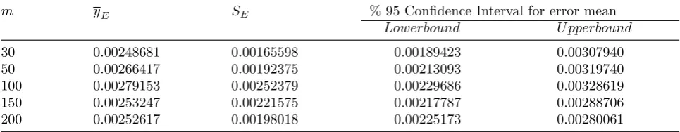
Table 4: Mean, standard deviation and mean confidence interval for error in Example5.2withn= 2 .
m yE SE % 95 Confidence Interval for error mean
Lowerbound U pperbound
30 0.00248681 0.00165598 0.00189423 0.00307940 50 0.00266417 0.00192375 0.00213093 0.00319740 100 0.00279153 0.00252379 0.00229686 0.00328619 150 0.00253247 0.00221575 0.00217787 0.00288706 200 0.00252617 0.00198018 0.00225173 0.00280061
Thus,yn(x) is referred to the nth-order
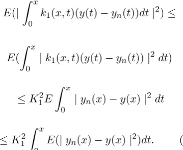
approxi-mation of the exact solutiony(x). By subtracting Eq. (2.1) from Eq. (4.10), we get
yn(x)−y(x) =
∫ x
0
k1(x, t)(y(t)−yn(t))dt+
∫ x
0
k2(x, t)(y(t)−yn(t))dWt. (4.11)
Since (a+b)2 ≤2a2+ 2b2 , we have
E(|yn(x)−y(x)|2)≤
2E(|
∫ x
0
k1(x, t)(y(t)−yn(t))dt|2)
+ 2E(|
∫ x
0
Table 5: Error between exact solution and approximate solution for Examples5.1and5.2withn= 1,2
x Example5.1 Example5.2
n= 1 n= 2 n= 1 n= 2
0.1 0.0000242909 0.0000142588 0.00036698 0.000631032 0.2 0.0001103250 0.0000693169 0.00004345 0.000444685 0.3 0.0004296230 0.0006350250 0.00126760 0.000039601 0.4 0.0006215360 0.0025920900 0.00434630 0.000880022 0.5 0.0000786668 0.0067937100 0.00989890 0.002060460
By using the Cauchy-Schwartz inequality, we ob-tain
E(|
∫ x
0
k1(x, t)(y(t)−yn(t))dt|2)≤
E(
∫ x
0
|k1(x, t)(y(t)−yn(t))|2 dt)
≤K12E
∫ x
0
|yn(x)−y(x)|2 dt
≤K12
∫ x
0
E(|yn(x)−y(x)|2)dt. (4.13)
Furthermore, from Theorem2.1, we can write
E(|
∫ x
0
k2(x, t)(y(t)−yn(t))dWt|2)≤
E(
∫ x
0
|k2(x, t)(y(t)−yn(t))|2 dt)
≤K22E
∫ x
0
|yn(x)−y(x)|2 dt
≤K22
∫ x
0
E(|yn(x)−y(x)|2)dt. (4.14)
Therefore, for some appropriate constant K we get
E(|yn(x)−y(x)|2)≤K
∫ x
0
E(
|(y(t)−yn(t))|2)dt. (4.15)
Thus, by using Granwall’s Lemma, we have E(| yn(x)−y(x)|2)→0 as n→ ∞.
5
Numerical examples
In this Section, we present numerical results for some examples from [11] to show the effi-ciency and the accuracy of the presented method.
Example 5.1 Consider the following linear stochastic Volterra integral equation,
y(x) =
1 +
∫ x
0
t2y(t)dt+
∫ x
0
ty(t)dWt, x, t∈[0,0.5),
(5.16)
with the exact solution y(x) = ex
3 6 +
∫x
0 tdWt, for
0 ≤ x < 0.5. The numerical results are shown in Tables 1 and 2. In the Tables, m is the number of iterations, yE is the error mean , and
sE is the standard deviation of error. Table 5
shows the error between the exact solution and the approximate solution for 0 ≤ x < 0.5 with
n= 1,2.
Example 5.2 Consider the following linear stochastic Volterra integral equation,
y(x) = 1 12+
∫ x
0
cos(t)y(t)dt+
∫ x
0
sin(t)y(t)dB(t)
x, t∈[0,0.5), (5.17)
with the exact solution y(x) =
1 12e−
x
4+sin(x)+
sin(2x) 8
∫x
0 sin(t)dB(t), for 0≤x <0.5. The numerical results are shown in Tables 3, 4
6
Conclusion
Because for some SDEs that can be written as Volterra integral equations, it is impossible to find the exact solution of Eq. (2.1). It would be con-venient to determine its numerical solution based on stochastic numerical analysis. This method is very simple and effective in comparison with other methods. Also, this method has least com-putations and cost comparing with other meth-ods. In this paper, the applicability and the ac-curacy of this method were shown by two exam-ples. The results of the numerical solution were compared with the analytical solution.
References
[1] M. H. Behzadi, M. Mirbolouki, Symmetric Error Structure in Stochastic DEA, Interna-tional Journal of Industrial Mathematics 4 (2012) 1-9.
[2] M. H. Behzadi, N. Nematollahi, M. Mir-bolouki, Ranking Efficient DMUs with Stochastic Data by Considering Inecient Frontier, International Journal of Industrial Mathematics 1 (2009) 219-226.
[3] M. A. Berger, V. J. Mizel,Volterra equations with Ito integrals I, Journal of Integral Equa-tions 2 (1980) 187-245.
[4] J. C. Cortes, L. Jodar, L. Villafuerte, Nu-merical solution of random differential equa-tions: a mean square approach, Mathemati-cal and Computer Modelling 45 (2007) 757-765.
[5] J.C. Cortes, L. Jodar, L. Villafuerte, Mean square numerical solution of random dif-ferential equations: facts and possibilities, Computers and Mathematics with Applica-tions 53 (2007) 1098-1106.
[6] H. Holden, B. Oksendal, J. Uboe, T. Zhang,Stochastic Partial Differential Equa-tions, second ed., Springer-Verlag, New York (2009).
[7] S. Jankovic, D. Ilic, One linear ana-lytic approximation for stochastic integro-differential eauations, Acta Mathematica Scientia 30B 4 (2010) 1073-1085.
[8] M. Khodabin, K. Maleknejad, M. Rostami, M. Nouri,Numerical solution of stochastic differential equations by second order Runge-Kutta methods, Mathematical and Computer Modelling 53 (2011) 1910-1920.
[9] M. Khodabin, K. Maleknejad, M. Rostami, M. Nouri, Interpolation solution in general-ized stochastic exponential population growth model, Applied Mathematical Modelling 36 (2012) 1023-1033.
[10] P. E. Kloeden, E. Platen,Numerical Solution of Stochastic Differential Equations, in: Ap-plications of Mathematics, Springer-Verlag, Berlin (1999).
[11] K. Maleknejad, M. Khodabin, M. Rostami,
Numerical solution of stochastic Volterra in-tegral equations by a stochastic operational matrix based on block pulse functions, Math-ematical and Computer Modelling (2011).
[12] M. G. Murge, B. G. Pachpatte, Succesive approximations for solutions of second or-der stochastic integrodifferential equations of Ito type, Indian Journal of Pure and Applied Mathematics 21 (3) (1990) 260-274 .
[13] M. G. Murge, B. G. Pachpatte, On sec-ond order Ito type stochastic integrodifferen-tial equations, Analele stiintifice ale Univer-sitatii. I. Cuzadin Iasi, Mathematica 25-34 (1984).
[14] B. Oksendal, Stochastic Differential Equa-tions, An Introduction with Applications, Fifth Edition, Springer-Verlag, New York (1998).
[16] X. Zhang, Euler schemes and large de-viations for stochastic Volterra equations with singular kernels, Journal of Differential Equations 244 (2008) 2226-2250 .
[17] X. Zhang, Stochastic Volterra equations in Banach spaces and stochastic partial differ-ential equation, Acta Journal of Functional Analysis 258 (2010) 1361-1425.
I was born on September 4, 1969 in the city of Karaj. I receipt high school diploma in 1988 on math-ematics branch. In 1989, I suc-cessfully passed the university en-trance exam and started my aca-demic studies on the statistics in the Shahid Beheshti University in Tehran. In 1994, I continue my studies at MS level on the statistics in the same university. In 1998, I be-came a member of the board of department of mathematics in Islamic Azad University Karaj branch. In 2000, I emprise to obtain my Ph.D. on statistics in Sciences Research University Tehran branch. I receipt my Ph.D. certification in 2004. My Ph. D. dissertation is entropy and statisti-cal hypothesis testing. During the years when I have taught in the university, I have written some scientific papers in scientific research in various fields and also I have supervised the theses of stu-dents at MS and Ph.D levels on different subjects. Also, I am Managing Editor of the International Journal of Mathematical Sciences. Now I am as-sociate professor in department of mathematics Islamic Azad University, Karaj branch.
Khosrow Maleknejad received his MS degree in Applied Mathemat-ics from Tehran University, Iran, in 1972 and his PhD degree in Nu-merical Analysis from the Univer-sity of Wales, Aberystwyth, UK in 1981. In September 1976, he joined the Faculty of the Basic Science, Department of Applied Mathematics at Iran University of
Sci-ence and Technology where he has been a Profes-sor since 2002. During 19912000, he also served as Vice-chair for graduate students. He was a Visiting Professor at the University of California at Los Angeles in 1990. His research interests in-clude numerical analysis in solving ill-posed prob-lems and solving Fredholm and Volterra integral equations. He has authored and coauthored more than 160 research papers on these topics. He is an Editor-in-chief of the International Journal of Mathematical Sciences and member of editorial board of some journals. He is a member of the AMS.