SOME ROBUST RIDGE ESTIMATORS: A COMPARATIVE STUDY.

[Badawairea* 6(12): December, 2019] ISSN 2349-4506

Impact Factor: 3.799

G

lobal

J

ournal of

E

ngineering

S

cience and

R

esearch

M

anagement

SOME ROBUST RIDGE ESTIMATORS: A COMPARATIVE STUDY

Abdulrasheed Bello Badawairea*, Kayode Ayindeb, M. L. Danyaroc, Umar A. Ahmedd

*

Department of Mathematics & Statistics, Federal University Wukari, Nigeria

Department of Statistics, Federal University of Technology Akure, Nigeria

Department of Basic Science,Yobe State College of Agriculture Gujba, Nigeria

Department of Basic Science,Taraba State College of Agriculture Jalingo, Nigeria

DOI: 10.5281/zenodo.3591003

KEYWORDS

:

Multicollinearity, Outlier(s), Robust Ridge, Robust Generalised Ridge.

ABSTRACT

In the presence of multicollinearity and outliers, the Ordinary Least Square estimator is found to be inefficient

due to the inflated standard errors. In this paper, some forms of Generalized Ridge regression parameters proposed

by Fayose and Ayinde (2019) were combined with robust estimators to estimate the parameters of linear regression

model when multicollinearity and outliers are jointly evident. Linear regression models with three and five

regressors (p = 3 and p = 5), three levels of multicololinearity (

𝜌 = 0.900, 0.990 𝑎𝑛𝑑 0.999)

, three levels of

percentages of outliers (

𝑛1% = 5%, 10% 𝑎𝑛𝑑 20%)

, three levels of magnitude of outliers (

𝜎

𝑜𝑢𝑡𝑙𝑖𝑒𝑟𝑠2

= 10,

100 𝑎𝑛𝑑 250)

and three levels of sample size

(𝑛 = 20, 40 𝑎𝑛𝑑 100)

were considered through Monte Carlo

experiments. The experiments were carried out 1000 times, and the performances of these combined estimators

and Ordinary Least Square were investigated and compared using the Mean Square Error (MSE) criterion. Results

show that the Maximum form of Fayose and Ayindes’ modified Generalized Ridge parameter of Troskie and

Chalton (1996) when combined with robust Least Absolute Deviation estimator (

𝛼̂

𝐿𝐴𝐷𝐹𝐴1𝑚𝑎𝑥

)

consistently performed

more efficiently than all other methods of parameter estimation of linear regression model considered. It also

shows that increasing the sample size, the number of explanatory variables, degree of multicollinearity, the

magnitude of outliers and percentage of outliers affect the efficiency of these estimators.

INTRODUCTION

Ordinary Least Squares (OLS) estimator is the most popular estimator used in estimating the parameters of the

linear regression model. This estimator is the Best Linear Unbiased Estimator when all the assumptions of the

Classical Linear Regression Model are met (Fonby, 1984; Maddala, 2002).

One of the problems encountered in regression analysis is the existence of outlier(s) in a dataset which is one of

the violations in the classical linear regression model. Outlier(s) renders the OLS residuals to be non-normal.

Consequently, the OLS estimator will be inefficient, and the estimates obtained from it will be imprecise as a

result of the inflated error variance (Ayinde et al., 2015). The following estimation techniques are developed to

handle the problems of outliers; M estimator proposed by Huber (1964), MM estimator proposed by Yohai (1987),

S estimator proposed by Rousseuw and Yohai (1984), LAD estimator proposed by Dielman (1984), LTS proposed

by Rousseuw, P. J. and Van Driessen, K. (1998). Different researchers such as Neykov and Neytchev (1991),

Atkinson and Weisberg (1991), Stronberg (1993), Rousseeuw and Van Driessen (1999), Agullo (2001), Jung

(2005), Li (2005), Cizek (2005) and Rousseeuw and Van Driessen (2006) also suggested different algorithms for

computing the LTS estimates.

[Badawairea* 6(12): December, 2019] ISSN 2349-4506

Impact Factor: 3.799

G

lobal

J

ournal of

E

ngineering

S

cience and

R

esearch

M

anagement

Multicollinearity and outlier problem can exist together in a dataset. Research works done to handle these

problems jointly includes robust M estimator for ridge regression proposed by Holland (1973), robust regression

methods based on M, MM, S, and GM estimators proposed by Samkar and Alpu (2010), ridge regression with M,

MM, S, LTS, LMS and LAD introduced by Lukman et al., (2014), Ridge Least Absolute Value Estimator

proposed by Pfaffenberger & Dielman (1990), Ridge MM estimator proposed by Habshah & Marina (2007), ridge

regression based on robust MM estimator for high dimensional data developed by Maronna (2011).

This article aims to investigate the performances of some ridge regression estimators when combined with some

robust regression estimators to combat the problems of outliers and multicollinearity in a linear regression model.

MATERIALS AND METHODS

Consider the standard linear regression model of the form:

𝑌 = 𝑋𝛽 + 𝑈

(1)

where

𝑌

is an n x 1 random vector of dependent variable,

𝑋

is an n x p matrix with full rank,

𝛽

is a p x 1 vector

of estimable parameters, and

𝑈

is an n x 1 random vector of residuals distributed as

𝑁(0, 𝜎

2

_𝐼

𝑛

)

. The Ordinary

Least Squares estimator of

𝛽

is

𝛽̂

𝑂𝐿𝑆

= (𝑋

′

𝑋)

−1

𝑋′𝑌

(2)

Let T be an orthogonal matrix, satisfying

𝑇

′

_𝑋

′

_{𝑋𝑇 = Λ = 𝑑𝑖𝑎𝑔(𝜆}

1

, 𝜆

2

, … , 𝜆

𝑝

)

, where

Λ

is a diagonal matrix of

order p x p with diagonal elements

𝜆

1

, 𝜆

2

, … , 𝜆

𝑝

as the eigen values of

𝑋

′

𝑋

. T and

Λ

are the matrices of eigen

vectors and eigen values, respectively. Hence, the canonical form of model (1) is:

𝑌 = 𝑍𝛼 + 𝑈

(3)

where

𝑍 = 𝑋𝑇

and

𝛼 = 𝑇′𝛽

.

Hence, the OLS estimator of

𝛼

is:

𝛼̂

𝑂𝐿𝑆

= Λ

−1

𝑍′𝑌

(4)

2.1 Robust Estimators

M Estimator

M-estimator proposed by Huber (1964) perform parameter estimation by minimizing the sum of a less rapidly

increasing function of the residuals. It performs better when the outliers are in the y-direction but less robust to

leverage. The objective function of M estimate is given by:

𝑚𝑖𝑛 ∑

𝜌 (

𝑈𝑖 𝑆

)

𝑛

𝑖=1

= 𝑚𝑖𝑛 ∑

𝜌 (

𝑌𝑖−𝑍′𝛼̂𝑖 𝑆

)

𝑛

𝑖=1

(5)

where s is the scale estimate obtained as function of residuals and is estimated by

𝑆 =

𝑚𝑒𝑑𝑖𝑎𝑛|𝑈𝑖−𝑚𝑒𝑎𝑑𝑖𝑎𝑛(𝑈𝑖)|

ℎ

(6)

When n is large, an appropriate choice of h makes S an approximately unbiased estimator of

𝜎

.

To minimize (5), a system of normal equations is solved by taking partial derivative with respect to

𝛽

and equating

them to zero, which gives

∑

𝑋

𝑖

𝜓 (

𝑌_𝑖−𝑍′𝛼̂_𝑖

𝑆

) = 0

𝑛

𝑖=1

(7)

Where

𝜓

is

𝜌

′

_and

_𝑍

𝑖

is the

𝑖

𝑡ℎ

observation. Then Iterative Reweighted Least Squares (IRLS) or nonlinear

optimization techniques is used to solve these equations.

MM-Estimator

[Badawairea* 6(12): December, 2019] ISSN 2349-4506

Impact Factor: 3.799

G

lobal

J

ournal of

E

ngineering

S

cience and

R

esearch

M

anagement

1.

Initial estimates

𝛼̂

(1)

_{found using a high breakdown point estimator are used to compute the initial}

residuals

𝑈

_𝑖(1)

.

2.

M-estimate of the scale of residuals

𝑆

𝑛

are computed using the initial estimate of residuals

𝑈

𝑖 (1)

in step 1.

3.

M-estimates of regression coefficients are obtained from Weighted Least Squares (WLS) whose first

iteration uses the residual scale

𝑆

𝑛

from step 2 and the estimates of residuals

𝑈

𝑖 (1)

from step 1

∑

𝑍

𝑖

𝑤

𝑖

(

𝑈_𝑖(1)

𝑆𝑛

) = 0

𝑛

𝑖=1

(8)

4.

Residuals from the initial Weighted Least Squares (WLS) in step 3 are used to construct new weights,

which again is used in Weighted Least Squares estimation. The process is continually reiterated until

convergence.

S-Estimator

S-estimator proposed by Rousseuw and Yohai (1984), is a high breakdown value that minimize the dispersion of

residuals. S-estimator minimize the dispersion in residuals as the solution of

1

𝑛

∑

𝜓 (

𝑈_𝑖

𝑠

)

𝑛

𝑖=1

= 𝐾

(9)

Where K is a constant.

Least Trimmed Squares Regression Estimator

Another estimator proposed by Rousseuw (1984), is the Least Trimmed Squares (LTS) regression. It is also a high

breakdown value method that minimizes the sum of the trimmed squared residuals. LTS estimator is

𝛼̂

𝐿𝑇𝑆

= 𝑎𝑟𝑔𝑚𝑖𝑛(∑

ℎ𝑖=1

𝑈

𝑖2

)

(10)

Where h is defined in the range

𝑛

2

+ 1 ≤ ℎ ≤

3𝑛+𝑃+1

4

, n and P representing sample size and number of parameters

in the model.

Least Absolute Deviation Estimator

Least Absolue Deviation (LAD) regression proposed by Dielman (1984) is very resistant to observations with

unusual Y values. Estimates are obtained by minimizing the sum of the absolute values of the residuals.

𝑚𝑖𝑛 ∑

𝑛𝑖=1

|𝑈

𝑖

|

= 𝑚𝑖𝑛 ∑

𝑛𝑖=1

|𝑌

𝑖

− 𝑍

𝑖

𝛼̂|

(11)

LAD fails to account for leverage (Mosteller and Turkey 1977), and thus has a breakdown point of zero.

Generalized Ridge Estimator

The Generalized Ridge estimator of

𝛼

is given by:

𝛼̂

𝐺𝑅

= [𝐼 − 𝐾(Λ + K)

−1

]𝛼̂

𝑂𝐿𝑆

(12)

Where

K = 𝑑𝑖𝑎𝑔(𝑘

1

, 𝑘

2

, … , 𝑘

𝑝

)

, is a p x p diagonal matrix whose elements

𝑘

1

, 𝑘

2

, … , 𝑘

𝑝

are the p different ridge

parameters corresponding to p different regressors considered. Therefore, the Generalized Ridge estimator of

𝛽

is

𝛽̂

𝐺𝑅

= 𝑇𝛼̂

𝐺𝑅

(13)

The mean square error of Generalized Ridge estimator is:

𝑀𝑆𝐸(𝛼̂

𝐺𝑅

) = 𝜎

2

∑

𝜆

𝑖

⁄

(𝜆

𝑖

+ 𝑘

𝑖

)

2

+

𝑝

𝑖=1

∑

𝑘

𝑖2

𝛼̂

𝑖2

⁄

(𝜆

𝑖

+ 𝑘

𝑖

)

2 𝑝

𝑖=1

(14)

While the MSE of

𝛼̂

𝑂𝐿𝑆

is given by:

[Badawairea* 6(12): December, 2019] ISSN 2349-4506

Impact Factor: 3.799

G

lobal

J

ournal of

E

ngineering

S

cience and

R

esearch

M

anagement

The generalized ridge parameters used in this study are those proposed by Fayose and Ayinde (2019).

Fayose and Ayinde (2019) proposed some generalized ridge parameters by taking the Minimum (MIN), Maximum

(MAX), Mid-Range (MID), Arithmetic Mean (AM), Median (MD), Geometric Mean (GM) and Harmonic Mean

(HM) of eigen values (

𝜆

𝑖

)

of

𝑋

′

𝑋

matrix to(of) the ridge parameter estimators proposed by Nomura (1988),

Troskie and chalton (1996), Firinguetti (1999), Batach

et. al

(2008), Dorugade (2016) and Lukman and Ayinde

(2017).

The estimators of generalized ridge parameters used in this study are the modification of Troskie and Chalton

(1996) and Firinguetti (1999) by Fayose and Ayinde. The generalize ridge parameter by Troskie and Chalton is:

𝑘

𝑇𝐶

= 𝜆

𝑖

𝜎

2

⁄

(𝜆

𝑖

𝛼̂

𝑖2

+ 𝜎

2

)

(16)

While that of Firinguetti is computed as:

𝑘

𝐹

= 𝜆

𝑖

𝜎

2

⁄

(𝜆

𝑖

𝛼̂

𝑖2

+ (𝑛 − 𝑝)𝜎

2

)

(17)

Where n is the sample size and p is the number of independent variables in the model.

Hence, the generalized ridge parameters used are:

𝑘

𝐹𝐴1𝑚𝑖𝑛

= 𝜆

𝑚𝑖𝑛

𝜎

2

⁄

(𝜆

𝑚𝑖𝑛

𝛼̂

𝑖2

+ 𝜎

2

)

(18)

Where

𝜆

𝑚𝑖𝑛

= minimum (

𝜆

𝑖

)

, i= 1, 2, …, p

𝑘

𝐹𝐴1𝑚𝑎𝑥

= 𝜆

𝑚𝑎𝑥

𝜎

2

⁄

(𝜆

𝑚𝑎𝑥

𝛼̂

2𝑖

+ 𝜎

2

)

(19)

Where

𝜆

𝑚𝑎𝑥

= maximum (

𝜆

𝑖

)

, i= 1, 2, …, p

𝑘

𝐹𝐴1𝑚𝑖𝑑

= 𝜆

𝑚𝑖𝑑

𝜎

2

⁄

(𝜆

𝑚𝑖𝑑

𝛼̂

𝑖2

+ 𝜎

2

)

(20)

Where

𝜆

𝑚𝑖𝑑

= (𝜆

𝑚𝑎𝑥

+ 𝜆

𝑚𝑖𝑛

) 2

⁄

𝑘

𝐹𝐴1𝑚𝑑

= 𝜆

𝑚𝑑

𝜎

2

⁄

(𝜆

𝑚𝑑

𝛼̂

𝑖2

+ 𝜎

2

)

(21)

Where

𝜆

𝑚𝑑

= median (

𝜆

𝑖

)

, i= 1, 2, …, p

𝑘

_𝐹𝐴1𝑔𝑚

= 𝜆

𝑔𝑚

𝜎

2

⁄

(𝜆

𝑔𝑚

𝛼̂

𝑖2

+ 𝜎

2

)

(22)

Where

𝜆

𝑔𝑚

= (𝜆

1

× 𝜆

2

×. . .× 𝜆

𝑝

)

1 𝑝

𝑘

𝐹𝐴1ℎ𝑚

= 𝜆

ℎ𝑚

𝜎

2

⁄

(𝜆

ℎ𝑚

𝛼̂

𝑖2

+ 𝜎

2

)

(23)

Where

𝜆

ℎ𝑚

= 𝑝 ∑

1 𝜆𝑖 𝑝 𝑖=1

⁄

.

Following a similar fashion, these forms are again applied to equation (17).

Robust Generalized Ridge Estimator

The robust generalized ridge estimator used in this study that jointly solve the problems of multicollinearity and

outliers is given by

𝛼̂

𝑅𝐺𝑅

= [𝐼 − 𝐾

𝑅𝑜𝑏𝑢𝑠𝑡𝐹𝐴

(Λ + 𝐾

𝑅𝑜𝑏𝑢𝑠𝑡𝐹𝐴

)

−1

]𝛼̂

𝑅𝑜𝑏𝑢𝑠𝑡

(24)

Where

𝐾

𝑅𝑜𝑏𝑢𝑠𝑡𝐹𝐴

are the Fayose and Ayindes’ generalized ridge parameters computed from robust (M, MM, S,

LTS, LMS and LAD) estimates instead of the usual OLS estimates, and

𝛼̂

𝑅𝑜𝑏𝑢𝑠𝑡

is the robust (M, MM, S, LTS,

LMS, LAD) estimator of the model parameters.

e.g,

𝑘

𝑅𝑜𝑏𝑢𝑠𝑡𝐹𝐴1𝑚𝑖𝑛

= 𝜆

𝑚𝑖𝑛

𝜎

𝑅𝑜𝑏𝑢𝑠𝑡2

⁄

(𝜆

𝑚𝑖𝑛

𝛼̂

𝑅𝑜𝑏𝑢𝑠𝑡𝑖2

+ 𝜎

𝑅𝑜𝑏𝑢𝑠𝑡2

)

(25)

𝑘

𝑅𝑜𝑏𝑢𝑠𝑡𝐹𝐴2𝑚𝑖𝑛

= 𝜆

𝑚𝑖𝑛

𝜎

𝑅𝑜𝑏𝑢𝑠𝑡2

⁄

(𝜆

𝑚𝑖𝑛

𝛼̂

𝑅𝑜𝑏𝑢𝑠𝑡𝑖2

+ (𝑛 − 𝑝)𝜎

𝑅𝑜𝑏𝑢𝑠𝑡2

)

.

(26)

Where equation (25) and (26) are the robust minimum forms of Fayose and Ayinde’s modified ridge parameters

of Troskie and Chalton (1996) and Firinguetti (1999) respectively.

[Badawairea* 6(12): December, 2019] ISSN 2349-4506

Impact Factor: 3.799

G

lobal

J

ournal of

E

ngineering

S

cience and

R

esearch

M

anagement

Simulation Study

In this paper, a Monte-Carlo experiment was carried out. The relation that yield the predictant is:

𝑌 = 𝑋𝛽 + 𝑈

(27)

The procedure adopted by [20] and Kibria (36) was used to generate the predictors, the procedure is:

𝑋

𝑡𝑖

= (1 − 𝜌

2

)

1

2

𝑍

_𝑡𝑖

+ 𝜌𝑍

_𝑡𝑝

(28)

Where

𝑍

𝑡𝑖

are the standard normal and independently distributed random variables, each with mean zero and unit

variance,

𝜌

is the degree of relationship between any two predictors, which is varied as

𝜌 = (0.900, 0.990, 0.999)

so as to study the effect of variation in degrees of multicollinearity.

The error term was simulated to have a Gaussian mixture, i.e.

𝑈

𝑡

~(1 − 𝑛1%)𝑁(0,1) + 𝑛1%𝑁(0, 𝜎

𝑜𝑢𝑡𝑙𝑖𝑒𝑟𝑠2

).

Where

𝑛1% = (5%, 10%, 20%)

were the percentages of outliers injected into the data, and

𝜎

𝑜𝑢𝑡𝑙𝑖𝑒𝑟𝑠2

= (10,

100, 250)

is the magnitude of outliers considered.

The number of predictors were varied as p = (3, 5) so as to study the impact of increase in number of predictors

in the model. When p = 3, the true parameter values were fixed as:

𝛽

1

= 0.8

,

𝛽

2

= 0.1

,

𝛽

3

= 0.6

, and when p =

5,

𝛽

1

= 0.6

,

𝛽

2

= 0.3

,

𝛽

3

= 0.2,

𝛽

4

= 0.15

and

𝛽

5

= 0.7

, such that

𝛽

′

𝛽 = 1

in both cases.

To investigate the impact of sample size on the performance of these estimators, three sample sizes were

considered, n = 20, 40, 100.

This experiment is replicated 1000 times and at each stage, the MSE is computed. The MSE of all the estimators

is average over the number of replications and parameters as:

𝐴𝑀𝑆𝐸(𝛽̂) =

1

1000

∑

∑

(𝛽̂

𝑖𝑗

− 𝛽

𝑖

)

2 1000

𝑗=1 𝑝

𝑖=1

.

(29)

This criterion was used in investigating the performances of these estimators.

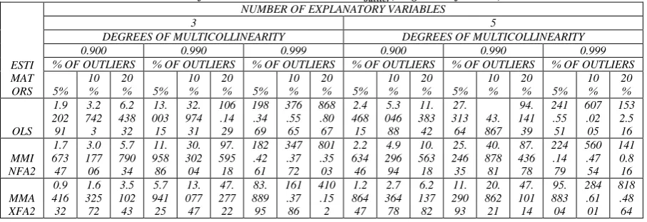
DISCUSSION OF RESULTS

The average of the estimated MSE of OLS and seventy-two (72) other robust generalized ridge estimators over

the number of parameters of a varying number of predictors at different sample sizes, the magnitude of outliers,

levels of multicollinearity and percentage of outliers are presented in Table 1 to Table 9 at the Appendix. From

Table 1 to Table 9, we observed that, at a fixed magnitude of outliers, number of explanatory variables, levels of

multicollinearity and percentage of outliers, as sample size increase, the AMSE of the estimators’ decreases. The

AMSE of the estimators increases with an increase in the magnitude of outliers.

Also, AMSE increases as the number of explanatory variables increase and as levels of multicollinearity increases.

𝛼̂

𝐿𝐴𝐷𝐹𝐴1𝑚𝑎𝑥

Consistently has the smallest values of AMSE, even though

𝛼̂

𝐿𝐴𝐷𝐹𝐴1𝑚𝑖𝑑

compete with it favourably. OLS

consistently has the largest values of AMSE, at all the levels of sample size, magnitude of outliers, number of

explanatory variables, levels of multicollinearity and percentage outliers considered.

CONCLUSSION

In this study, the performances of some forms of Generalized Ridge parameters proposed by Fayose and Ayinde

(2019) when combined with Robust estimators to jointly combat the problems of multicollinearity and outliers

were evaluated and compared using the MSE criterion.

[Badawairea* 6(12): December, 2019] ISSN 2349-4506

Impact Factor: 3.799

G

lobal

J

ournal of

E

ngineering

S

cience and

R

esearch

M

anagement

REFERENCES

1.

Agullo, J. (2001), ‘New algorithms for computing the least trimmed squares regression estimator’,

Computational Statistics and Data Analysis

36(4), 425–439.

2.

Atkinson, A. & Weisberg, S. (1991), simulated annealing for the detection of multiple outliers using

least squares and least median of squares fitting,

in

W. Stahel & S. Weisberg, eds, ‘

Directions in Robust

Statistics and Diagnostics’

, Springer-Verlag, New York.

3.

Ayinde, K., Lukman, A. F.

and Arowolo, O.T. (2015). Robust regression diagnostics of influential

observations in linear regression model.

Open Journal of Statistics

, 5, 1-11.

4.

Batah, F., Ramanathan, T. and Gore, S. (2008). The efficiency of modified Jacknife and Ridge Type

Regression Estimators: A Comparison, Surveys in Mathematics and its Applications, 24(2),

F.

157 – 174.

5.

Belsley, D. A., Kuh, E., & Welsch, R. E. (1980). Regression Diagnostics: Identifying Influential Data

and Sources of Collinearity.

Wiley Series in probability and Mathematical Statistics

. New York: John

Wiley & Sons.

6.

Chatterjee, S. and Hadi, A.S. 2006. Regression by Example. 4

th

_{Edition, A Wiley-Interscience}

Publication, John Wiley and Sons.

7.

Chatterjee, S., Hadi, A.S. and Price, B. 2000. Regression by Example. 3

rd

_{Edition, A Wiley-Interscience}

Publication, John Wiley and Sons.

8.

Cizek, P. (2005), ‘Least trimmed squares in nonlinear regression under dependence’,

Journal of

Statistical Planning and Inference

136(11), 3967–3988.

9.

Dorugade, A. V. (2014). New Ridge Parameters for Ridge Regression. Journal of the Association of

Arab Universities for Basic and Applied Sciences, 15(1), 94 – 99.

10.

Firinguetti, L. A (1999). Generalized Ridge Regression Estimator and its Finite Sample Properties.

Communications in Statistics. Theory and Methods 28(5), 1217 – 1229.

11.

Fomby, T. B., Hill, R. C. and Johnson, S. R. 1984. Advance Econometric Methods. Springer-Verlag,

New York, Berlin, Heidelberg, London, Paris,Tokyo.

12.

Habshah Midi & Marina Zahari. “A Simulation Study on Ridge Regression Estimators in the Presence

of Outliers and Multicollinearity.”

Jurnal Teknologi

. 47(C): 59-74, 2007.

13.

Helland I. S. 1990. Partial least squares regression and statistical methods. Scandinavian Journal of

Statistics, 17, 97 – 114.

14.

Holland, P. W. (1973). Weighted ridge regression: Combining ridge and robust regression methods.

NBER Working Paper Series 11, 1-19.

15.

Hoerl, A. E. & Kennard, R.W. "Ridge Regression Biased Estimation for Nonorthogonal

Problems",

Technometrics

,Vol.12, 55-67, 1970.

16.

Huber, P. H. 1964. ‘‘Robust estimation of location parameter.’’ The Annals of Mathematical Statistics,

35 7 101.

17.

Jung, K. (2005), ‘Multivariate least-trimmed squares regression estimator’,

Computational Statistics and

Data Analysis

48(2), 307–316.

18.

Li, L. (2005), ‘An algorithm for computing exact least-trimmed squares estimate of simple linear

regression with constraints’,

Computational Statistics and Data Analysis,

48(4), 717–734.

19.

Lukman, A.F, Arowolo, O. and Ayinde, K. (2014). Some robust ridge regression for handling

multicollinearity and outlier. International Journal of Sciences: Basic and Applied Research 16(2),

192-202.

20.

Lukman, A.F, and Ayinde, K. (2017). Review and Classifications of the Ridge Parameter Estimation

Techniques. Haccetteppe Journal of Mathematics and Statistics, 46 (5), 953 – 967.

21.

Lukman, A. F., Ayinde, K., Binuomote, S. and Onate, A. C., (

2019

). Modified ridge‐type estimator to

combat multicollinearity: Application to chemical data

. Journal of Chemometrics

, e3125.

22.

Maddala, G. S. 2002. Introduction to Econometrics. 3

rd

_{Edition, John Willey and Sons Limited, England.}

23.

Maronna, R.A. “Robust Ridge Regression for High-Dimensional Data.”

Technometrics

, 53(1): 44- 53,

2011.

24.

Massy, W.F. (1965). Principal Components Regression in exploratory statistical research. J. Am. Stat.

Assoc., 60, 234-256.

[Badawairea* 6(12): December, 2019] ISSN 2349-4506

Impact Factor: 3.799

G

lobal

J

ournal of

E

ngineering

S

cience and

R

esearch

M

anagement

26.

Neykov, N. & Neytchev, P. (1991), ‘Least median of squares, least trimmed squares and S estimations

by means of BMDP3R and BMDPAR’,

Computational

Statistics Quarterly

4, 281–293.

27.

Nomura, M. (1988). On the Almost Unbiased Ridge Regression Estimator. Communication in Statistics

– Simulation and Computation, 17(3), 729 – 743.

28.

Pfaffenberger, R. C., & Dielman, T. E. “A comparison of regression estimators when both

multicollinearity and outliers are present.” In

Robust regression:Analysis and applications

, K. Lawrence

& J. Arthur (Eds.), 243-270. New York: Marcel Dekker, 1990.

29.

Phatak, A. and Jony, S. D. 1997. The geometry of partial least squares. Journal of Chemometrics, 11,

311 – 338.

30.

Rousseeuw, P. J. & van Driessen, K. (1999), ‘A fast algorithm for the minimum covariance determinant

estimator’,

Technometrics

41(3), 212–223.

31.

Rousseeuw, P. & van Driessen, K. (2006), ‘Computing LTS regression for large data sets’,

Data Mining

and Knowledge Discovery

12(1), 29–45.

32.

Rousseeuw p. j., and Yohai, 1984. ‘‘Robust regression by means of S estimators in Robust and Nonlinear

Time Series Analysis’’, Franke J. Hardle, W. and Martin, R. D. Lecture Notes in Statistics, 26, New

York: Springer-Verlag 256 - 274.

33.

Rousseeuw, P. J. and Van Driessen K., ‘‘Computing LTS for Large Data Sets.’’ Technical Report,

University of Antwerp, submitted, 1998.

34.

Samkar, H. and Alpu, O. (2010). Ridge regression based on some robust estimators. Journal of Modern

Applied Statistical Methods: 9(2), 495-501.

35.

Stein, C. M. (1960). Multiple Regression, Contributions to Probability and Statistics, Stanford

University Press, 424-443.

36.

Stromberg, A. (1993), ‘Computing the exact least median of squares estimate and stability diagnostics

in multiple linear regression’,

SIAM Journal on Scientific Computing

14(6),

1289–1299.

37.

Taiwo, S. F. and Kayode Ayinde (2019). Different Forms Biasing Parameter for Generalized Ridge

Regression Estimator. International Journal of Computer Applications, 181(37), 0975 – 8887.

38.

Tibshirani, R. (1996).

Regression shrinkage and selection via the LASSO

. J. Royal. Statist. Soc B., Vol.

58, No. 1, p 267-288).

39.

Troskie, C. G. and Chalton, D. O. (1996). A Bayesian Estimate for the Constants in Ridge Regression.

South African Statistical Journal, 30, 119 – 137.

40.

Yohai, V. J. ‘‘High breakdown point and high efficiency robust estimates for regression.’’ The Annals

of Statistics, 15, 642 – 656, 1987.

41.

Wold, H. (1966). Estimation of Principle Components and Related Models by Iterative Least Squares.

In P. R. Krishnaiaah (Ed.). Multivariate Analysis. (pp.391420) New York, Academic Press.

APPENDIX

Table 1: AMSE of the estimators when n = 20 and 𝝈𝒐𝒖𝒕𝒍𝒊𝒆𝒓𝟐 ( magnitude of outliers) = 10

ESTI MAT ORS

NUMBER OF EXPLANATORY VARIABLES

3 5

DEGREES OF MULTICOLLINEARITY DEGREES OF MULTICOLLINEARITY

0.900 0.990 0.999 0.900 0.990 0.999

% OF OUTLIERS % OF OUTLIERS % OF OUTLIERS % OF OUTLIERS % OF OUTLIERS % OF OUTLIERS

5% 10 %

20

% 5%

10 %

20

% 5%

10 %

20

% 5%

10 %

20

% 5%

10 %

20

% 5%

10 %

20 %

OLS 1.9 202 91

3.2 742 3

6.2 438 32

13. 003 15

32. 974 31

106 .14 29

198 .34 69

376 .55 65

868 .80 67

2.4 468 15

5.3 046 88

11. 383 42

27. 313 64

43. 867

94. 141 39

241 .55 51

607 .02 05

153 2.5 16

MMI NFA2

1.7 673 47

3.0 177 06

5.7 790 34

11. 958 86

30. 302 04

97. 595 18

182 .42 61

347 .37 72

801 .35 03

2.2 634 46

4.9 296 94

10. 563 18

25. 246 35

40. 878 81

87. 436 78

224 .14 79

560 .47 54

141 0.8 16

MMA XFA2

0.9 416 32

1.6 325 72

3.5 102 43

5.7 941 25

13. 077 47

47. 277 22

83. 889 95

161 .37 86

410 .15 2

1.2 864 47

2.7 364 78

6.2 137 82

11. 290 93

20. 862 21

47. 101 14

95. 883 04

284 .61 01

[Badawairea* 6(12): December, 2019] ISSN 2349-4506

Impact Factor: 3.799

G

lobal

J

ournal of

E

ngineering

S

cience and

R

esearch

M

anagement

MMI DFA2

1.0 506 62

1.7 775 99

3.7 609 4

5.9 635 05

13. 221 88

47. 821 83

83. 991 75

161 .71 46

410 .63 37

1.3 841 77

2.9 379 98

6.4 282 57

11. 349 54

21. 054 58

47. 422 67

95. 969 41

284 .73 8

818 .73 43

MMF A2

1.6 093 1

2.6 953 13

5.4 253 32

11. 351 34

26. 427 17

82. 010 56

159 .61 79

327 .41 81

710 .05 7

2.0 385 35

4.1 709 41

8.8 682 4

21. 831 84

36. 899 91

69. 320 83

186 .65 23

437 .69 29

103 1.2 92

MGM FA2

1.4 497 41

2.4 310 05

4.8 909 83

9.0 729 7

19. 665 86

65. 757 4

106 .81 28

218 .88 22

504 .25 14

1.9 913 35

4.0 857 6

8.5 163 66

15. 423 66

28. 339 96

57. 475 73

109 .32 78

304 .35 02

849 .11 99

MHM FA2

1.7 535 82

2.9 469 29

5.6 486 14

12. 768 1

32. 577 09

105 .28 94

198 .12 74

376 .14 11

867 .97 13

2.3 184 06

5.0 423 96

10. 892 91

27. 159 39

43. 582 28

93. 660 36

241 .40 72

606 .70 1

153 1.9 49

MMI NFA1

1.1 221 67

1.9 814 48

4.0 401 87

7.6 459 53

18. 826 8

64. 120 16

117 .22 33

223 .31 27

540 .91 44

1.5 801 98

3.5 067 29

7.8 248 79

16. 837 99

29. 041 8

64. 269 45

151 .91 09

396 .43 43

104 5.0 39

MMA XFA1

0.8 146 81

1.4 684 02

3.2 264 69

5.6 436 13

12. 945 76

46. 778 84

83. 795

161 .06 49

409 .69 73

1.1 794 39

2.5 025 8

5.9 917 45

11. 237 83

20. 688 93

46. 811 09

95. 803 09

284 .49 15

818 .25 62

MMI DFA1

0.8 221 23

1.4 783 33

3.2 437 59

5.6 524 22

12. 953 8

46. 809 44

83. 800 9

161 .08 44

409 .72 67

1.1 866 88

2.5 191 65

6.0 073 37

11. 241 56

20. 700 99

46. 831 41

95. 808 78

284 .49 99

818 .27 26

MMF A1

0.9 514 36

1.6 715 38

3.6 570 95

6.8 676 7

15. 083 92

51. 891 71

95. 959 9

196 .99 21

458 .51 2

1.3 424 96

2.7 945 62

6.4 836 74

13. 240 07

24. 219 94

50. 494 69

113 .16 38

308 .00 32

848 .74 16

MGM FA1

0.8 830 23

1.5 730 12

3.4 136 94

5.9 317 09

13. 441 87

48. 322 04

85. 210 27

164 .71 48

415 .74 69

1.3 168 82

2.7 584 3

6.3 635 95

11. 561 09

21. 359 94

47. 776 74

96. 634 54

285 .75 42

820 .32 59

MHM FA1

1.0 859 87

1.8 396 97

3.8 229 42

10. 495 71

28. 063 31

94. 883 8

194 .78 08

369 .82 38

855 .20 36

1.6 754 39

3.6 609 99

8.3 022 38

25. 370 91

40. 436 33

88. 188 67

239 .38 91

602 .34 4

152 4.1 73 MM

MINF A2

1.7 596 34

2.9 985 51

5.7 208 6

11. 895 57

30. 128 87

96. 778 34

181 .48 3

344 .75 09

793 .65 17

2.2 464 02

4.8 929 38

10. 436 4

25. 117 06

40. 561 22

86. 404 39

222 .88 15

554 .67 1

138 8.9 58 MM

MAX FA2

0.7 635 57

1.1 139 97

2.1 021 14

4.1 904 65

7.8 009 62

23. 596 61

57. 924 43

95. 081 6

190 .42 46

0.9 150 36

1.8 079 71

3.0 077 07

7.4 559 75

11. 487 36

22. 783 02

64. 755 68

160 .79 14

338 .06 6 MM

MID FA2

0.9 002 49

1.3 202 51

2.5 416 09

4.4 040 01

7.9 936 95

24. 351 43

58. 048 66

95. 504 6

191 .11 13

1.0 545 43

2.1 168 37

3.4 045 04

7.5 320 91

11. 768 46

23. 284 27

64. 863 43

160 .97 11

338 .46 41 MM

MFA 2

1.5 817 29

2.6 068 2

5.2 565 5

11. 206 9

25. 564 59

76. 443 28

155 .03 92

320 .96 87

672 .55 57

1.9 684 04

3.9 204 41

7.8 627 79

21. 150 3

35. 532 73

59. 598 13

179 .14 5

388 .28 97

738 .80 75 MMG

MFA 2

1.3 936 21

2.2 556 54

4.4 651 25

8.4 362 77

16. 875 79

52. 122 66

87. 744 47

176 .11 56

346 .88 98

1.9 067 66

3.8 031 05

7.2 522 19

12. 993 24

23. 225 17

40. 122 71

82. 339 03

190 .28 48

393 .93 69 MMH

MFA 2

1.7 445 97

2.9 191 36

5.5 610 33

12. 764 23

32. 572 83

105 .28 11

198 .12 72

376 .14 04

867 .97 01

2.3 101 52

5.0 25

10. 853 14

27. 158 36

43. 579 22

93. 655 32

241 .40 71

606 .70 07

153 1.9 49 MM

MINF A1

0.9 901 03

1.6 163 75

3.0 358 72

6.5 993 28

15. 751 41

49. 565 53

101 .42 86

182 .38 1

408 .38 52

1.3 371 8

2.9 733 12

6.0 057 89

14. 853 67

24. 294 06

51. 359 05

136 .69 69

328 .09 94

765 .56 67 MM

MAX FA1

0.6 113 65

0.8 992 14

1.6 488 83

4.0 070 52

7.6 309 63

22. 941 53

57. 808 84

94. 689 71

189 .78 7

0.7 696 38

1.4 617 77

2.6 231 45

7.3 878 07

11. 244 56

22. 352 73

64. 656 2

160 .62 53

337 .69 93 MM

MID FA1

0.6 195 72

0.9 107 81

1.6 727 05

4.0 175 17

7.6 411 33

22. 980 07

57. 816 02

94. 714

189 .82 67

0.7 788 49

1.4 842 99

2.6 476 77

7.3 925 63

11. 261 04

22. 381 74

64. 663 27

160 .63 71

337 .72 54 MM

MFA 1

0.7 757 74

1.1 686 48

2.3 581 38

5.5 803 83

10. 606 26

30. 427 81

73. 455 2

144 .92 12

269 .38 09

0.9 947 14

1.8 969 52

3.5 080 51

10. 075 08

16. 775 43

28. 409 51

87. 368 43

195 .82 57

393 .22 96 MMG

MFA 1

0.6 913 09

1.0 322 58

1.9 384 52

4.3 635 51

8.2 948 57

25. 066 35

59. 557 43

99. 400 87

198 .72 62

0.9 581 58

1.8 415 73

3.2 840 2

7.8 115 04

12. 230 08

23. 853 43

65. 701 83

162 .41 56

[Badawairea* 6(12): December, 2019] ISSN 2349-4506

Impact Factor: 3.799

G

lobal

J

ournal of

E

ngineering

S

cience and

R

esearch

M

anagement

MMH MFA 1

0.9 451 68

1.4 308 24

2.6 744 84

10. 196 87

27. 545 3

93. 636 22

194 .72 52

369 .66 69

854 .89 24

1.4 815 39

3.1 970 93

7.0 025 14

25. 245 25

40. 083 79

87. 545 68

239 .36 69

602 .28 09

152 4.0 73

SMIN FA2

1.7 700 2

3.0 089 4

5.7 320 37

11. 973 98

30. 267 15

96. 944 68

182 .18 95

346 .56 14

795 .15 64

2.2 589 38

4.9 056 66

10. 461 63

25. 241 73

40. 769 47

86. 585 14

224 .15 32

556 .55 91

139 1.5 42

SMA XFA2

0.9 521 96

1.3 408 53

2.3 521 87

5.7 988 36

11. 207 73

27. 508 2

75. 429 88

140 .28 3

227 .29 81

1.1 604 29

2.1 895 21

3.5 724 02

10. 704 22

16. 809 76

27. 085 02

99. 019 65

213 .04 67

418 .95 38

SMID FA2

1.0 604 22

1.5 208

2.7 581 32

5.9 688 44

11. 366 59

28. 225 14

75. 539 58

140 .64 86

227 .93 64

1.2 706 92

2.4 538 66

3.9 433 42

10. 768 76

17. 039 66

27. 562 11

99. 109 06

213 .20 39

419 .32 02

SMF A2

1.6 155 68

2.6 507 52

5.2 878 48

11. 379

26. 218 5

77. 453 17

158 .27 37

325 .51 3

679 .69 01

2.0 160 31

4.0 151 91

8.0 516 52

21. 807 77

36. 395 32

61. 417 54

187 .62 54

406 .74 15

786 .53 05

SGM FA2

1.4 584 39

2.3 383 6

4.5 419 82

9.1 212 96

18. 839

54. 437 74

100 .49 23

205 .88 55

373 .49 08

1.9 637 21

3.9 110 81

7.4 888 37

15. 169 5

26. 215 44

43. 340 59

112 .55 95

237 .84 43

470 .34 03

SHM FA2

1.7 555 42

2.9 327 92

5.5 770 95

12. 768 83

32. 576 01

105 .28 29

198 .12 74

376 .14 08

867 .97 03

2.3 167 57

5.0 315 63

10. 860 5

27. 159 1

43. 581

93. 656 28

241 .40 72

606 .70 08

153 1.9 49

SMIN FA1

1.1 319 47

1.7 787 51

3.2 144 31

7.6 791 42

17. 893 51

52. 024 66

112 .01 38

210 .92 03

431 .21 54

1.4 960 8

3.1 878 11

6.3 440 89

16. 663 09

27. 083 84

53. 785 69

154 .21 7

354 .60 4

810 .93 17

SMA XFA1

0.8 334 55

1.1 520 89

1.9 292 95

5.6 492 65

11. 069 2

26. 883 15

75. 327 57

139 .94 27

226 .70 46

1.0 465 47

1.8 896 52

3.2 096 46

10. 645 73

16. 607 4

26. 671 12

98. 936 78

212 .90 11

418 .61 63

SMID FA1

0.8 396 57

1.1 623 81

1.9 519 51

5.6 579 41

11. 077 43

26. 920 05

75. 333 92

139 .96 37

226 .74 16

1.0 536 58

1.9 096 5

3.2 329 91

10. 649 84

16. 621 28

26. 699 21

98. 942 68

212 .91 15

418 .64 03

SMF A1

0.9 618 39

1.3 885 87

2.5 887 79

6.8 867 54

13. 561 99

33. 968 75

88. 539 02

180 .86 25

300 .86 86

1.2 233 3

2.2 657 55

4.0 398 28

12. 830 4

21. 026 94

32. 377 05

116 .37 33

242 .47 26

469 .68 92

SGM FA1

0.8 953 47

1.2 693 32

2.2 005 23

5.9 368 37

11. 617 01

28. 902 65

76. 852 88

143 .95 78

235 .00 99

1.1 944 46

2.2 183 22

3.8 309 27

11. 001 48

17. 411 94

28. 100 44

99. 794 39

214 .45 68

421 .73 4

SHM FA1

1.0 948 51

1.6 102 6

2.8 792 26

10. 523 18

27. 905 59

93. 875 26

194 .76 75

369 .76 73

854 .94 97

1.6 139 96

3.3 821 31

7.2 353 74

25. 341 85

40. 289 5

87. 652 04

239 .38 69

602 .30 26

152 4.0 83 LTSM

INFA 2

1.7 876 24

3.0 399 86

5.7 847

12. 109 72

30. 581 17

97. 987 47

183 .95 39

350 .63 62

802 .43 13

2.2 953 54

4.9 767 96

10. 611 34

25. 603 48

41. 374 33

87. 850 77

227 .31 18

566 .71 55

141 4.7 2 LTSM

AXFA 2

1.1 779 56

1.8 262 82

3.2 934 13

7.5 462 74

16. 536 68

46. 776 47

105 .69 76

204 .23 96

391 .26 97

1.6 196 19

3.2 740 44

6.2 058 89

16. 064 77

26. 151 6

49. 795

147 .74 4

360 .77 89

794 .07 41 LTSM

IDFA 2

1.2 548 66

1.9 525 69

3.5 723 27

7.6 714 84

16. 656 85

47. 311 57

105 .77 31

204 .50 07

391 .75 64

1.6 827 56

3.4 277 01

6.4 246 02

16. 104 15

26. 298 94

50. 106 28

147 .80 01

360 .87 35

794 .30 94

LTSM FA2

1.6 640 43

2.7 597 6

5.4 218 89

11. 639 92

27. 415 82

82. 763 58

164 .97 46

334 .31 29

710 .78 77

2.1 299 23

4.3 698 29

8.9 520 85

23. 175 12

38. 365 51

71. 171 74

202 .73 97

473 .65 79

101 7.8 34 LTSG

MFA 2

1.5 442 24

2.5 294 38

4.8 481 38

9.9 561 42

22. 028 5

65. 985 05

122 .80 75

249 .35 71

492 .69 84

2.0 963 12

4.3 036 48

8.5 923 2

18. 850 91

31. 957 84

60. 051 23

156 .24 02

375 .71 53

825 .44 85 LTSH

MFA 2

1.7 760 17

2.9 783 03

5.6 576 05

12. 780 86

32. 587 44

105 .30 11

198 .12 82

376 .14 26

867 .97 21

2.3 379 68

5.0 718 05

10. 920 22

27. 164 04

43. 592 55

93. 668 58

241 .40 79

606 .70 19

153 1.9 5 LTSM

INFA 1

1.3 059 39

2.1 327 4

3.8 896 32

8.9 128 89

21. 352 28

64. 261 23

130 .93 07

252 .81 25

532 .40 41

1.8 128 25

3.8 595 64

7.8 766 76

19. 801 24

32. 491 32

66. 487 79

181 .93 7

443 .68 85

103 2.8 85 LTSM

AXFA 1

1.0 944 44

1.6 913 64

3.0 016 62

7.4 356 69

16. 430 05

46. 295 61

105 .62 72

203 .99 61

390 .81 56

1.5 535 74

3.0 991 55

5.9 910 98

16. 029 19

26. 020 46

49. 519 74

147 .69 19

360 .69 12