Improvement of Localization Algorithm for Wireless Sensor Networks Based on DV-Hop

Improvement of Localization Algorithm for Wireless

Sensor Networks Based on DV-Hop

https://doi.org/10.3991/ijoe.v15i06.9681

Xin Qiao

Chaohu University, Anhui, China

Fei Chang(*₎

Inspur Group Company Limited, Shandong, China

[email protected]

Jing Ling

Chaohu University, Anhui, China

Abstract—DV-Hop localization algorithm is a typical representative of range-free algorithms, which can be applied to large-scale wireless sensor net-work location monitoring with random distribution of nodes, such as geological hazard monitoring, water pollution monitoring, forest fire monitoring and more. In order to get a higher positioning accuracy, a new method is used to determine the average hop distance of anchor nodes firstly. Secondly, the estimated dis-tances between nodes are calculated by using the correction value correspond-ing to the average hop distance; finally, in the positioncorrespond-ing stage, when the num-ber of anchor nodes is small, the Min-Max (Minimum-Maximum) method is used to obtain the estimated coordinates; on the contrary, the ML (Maximum Likelihood) method is used to calculate the estimated coordinates. One is to re-duce the amount of calculation; the other is to keep the accuracy stable. Finally, the Quasi-Newton method is used to iteratively optimize the coordinates of un-known nodes. The results indicate that the accuracy of algorithm is about 15%-20% higher than that of the original DV-Hop algorithm.

Keywords—Min-max method, localization, quasi newton method

1

Introduction

WSNs (Wireless sensor networks) are widely used in various fields because of its convenient data collection and transmission, and simple networking. However, in any field, all kinds of information associated with data are indispensable, and location information is the most important of this information [1]. Therefore, location technol-ogy is a hot and difficult point in the research of wireless sensor networks, and it is the basis of acquiring various monitoring objects information [2].

algorithm [6], DV-Hop algorithm and more [7]. Range-based localization algorithm requires high hardware equipment and multiple measurements to obtain reasonable positioning accuracy, so the computation and communication costs are very high. Compared with the ranging-free algorithm, the location method is simple, does not need additional hardware equipment, and has less communication overhead. There-fore, this location method has attracted more and more attention. Among them, DV-Hop has many advantages in rang-free algorithm and is widely used in large WSN [8].

DV-Hop is a range-free algorithm that does not require additional hardware to lo-cate only according to network connectivity. It is a coarse-grained estimation and localization algorithm. At present, experts and scholars at home and abroad have tried to improve the DV-Hop algorithm, and a lot of research work has been done. The localization accuracy is much higher than that of traditional algorithm. Liu Yan-hong and Liu Bing-ri of Jilin University proposed to replace the one-hop distance of anchor node in DV-Hop algorithm with RSSI ranging technology and to use hyperbola meth-od instead of trilateral measurement to achieve positioning [9]. To a certain extent, the positioning accuracy has been greatly improved. Su Kai and Cao Yuan of Nanjing University put forward a hybrid location system based on UWB and DGPS [10]. Lin Jin-chao of Chongqing University of Posts and Telecommunications uses Taylor series method to iteratively refine the coordinates of unknown nodes by calculating the initial values of the location results obtained by least square method [11]. The above improvements only improve the DV-Hop algorithm step by step without con-sidering its location accuracy. This paper mainly improves the DV-Hop algorithm from two aspects and simulates the comprehensive improvement. Compared with the original algorithm, the positioning accuracy and stability of the proposed algorithm are greatly improved.

2. DV-Hop Algorithm Description

The positioning process is as follows:

Step 1: Distance vector switching protocol: According to the distance vector

routing switching protocol, anchor nodes send packets to all other nodes in the net-work.

Step 2: Calculate the average hop and the distance: After obtaining the

coordi-nates and hops of other anchor nodes, the average hop distance of each anchor node is calculated by formula 1. Through the second flooding method, all the obtained anchor node information and the average hop distance are sent to the network. In order to ensure that the unknown node receives the average hop distance of the nearest anchor node, only the first received average hop distance is saved.

(1)

, 1 2

( )

N

ij ij j i i

i

ij

h d HS

h

¹ =

*

Among them, and is the coordinate between . is the minimum hop( ). When the average hop distance of anchor node is obtained from formula 1, the estimated distance can be obtained by average hop distance and hop count [12].

Step 3 Positioning stage: The estimated distance between anchor node and

un-known node is obtained by the second stage, so it can be solved by node coordinate estimation algorithm.

2

Improved Algorithm-CNDV-Hop (Corrected Quasi Newton

DV-Hop)

In this paper, CNDV-Hop algorithm is simulated from the following two aspects and the positioning accuracy are greatly improved.

2.1 Improved average hopping distances

The traditional algorithm makes the unbiased estimation criterion calculate the av-erage distance per hop. However, in random distributed wireless sensor networks, the estimation error of average hop distance is Gaussian distribution, and it is reasonable to use mean square error to estimate the average hop distance [13]. Therefore, the minimum mean square error criterion is used to calculate the distance instead of the unbiased estimation criterion.

Namely,

(2)

Let , the average hop distance of anchor node can be re-represented

as:

(3) The average hop distance can be recalculated by formula 1，the minimum hop

number between and are three hops; between are three hops, and between are six hops. The average hop distance are:

2 2

( ) ( )

ij i j i j

d = x x- + y y- ( , ),( , )x y_{i i} x y_{j j}

,

i j

h

i j

¹

2

(

)

j i

f

d

HS h

¹

=

å

-

×

0

i

f

HS

¶

=

¶

i

, 1 2

(

)

N

ij ij j i i

i

ij

h d

HS

h

¹ =

*

=

å

i

j

j k

,

,

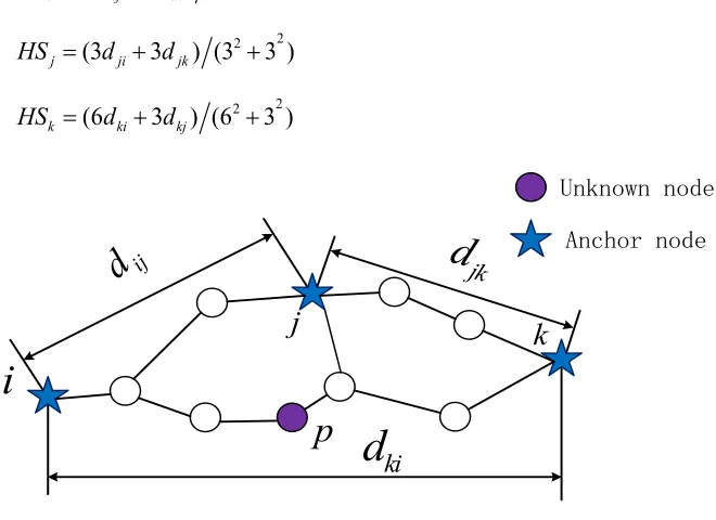
Fig. 1. Network topology diagram

In the second phase, the unknown node regards the first anchor node’s average hop distance as its own. Considering the hop distance information of multiple anchor nodes, the positioning accuracy can be improved [14]. The number of anchor nodes that can communicate with unknown nodes is k, and the average hop correction for k anchor nodes is:

(4) Combined with formula (4), the improved average hop distance is as follows:

(5) In the formula, the improved average hop distance will be closer to the actual aver-age hop distance of the whole network if the anchor node participates in the modifica-tion and improvement of calculating the average hop distance.

From the above conclusions and combined with Figure 1, the average hop distance

of the improved anchor nodes are:

2 2

(3

6 ) (3 6 )

i ij ik

HS

=

d

+

d

+

2 2

(3

3 ) (3 3 )

j ji jk

HS

=

d

+

d

+

2 2

(6

3 ) (6 3 )

k ki kj

HS

=

d

+

d

+

Unknown node

Anchor node

p

k

j

i

ij

d

d

ki

d

1

i k i i

HS

k

v

=

=

=

å

'

2

i i

HS

HS

=

+

v

, , Therefore,

to the anchor nodes are estimated to be: ,

and .

2.2 Improvement of positioning calculation

Performance comparison between ML algorithm and Min-Max algorithm:

Traditional position calculation methods mostly use trilateral location method or ML algorithm to obtain coordinates [12]. Trilateral location method is simple in calcula-tion and low in posicalcula-tioning accuracy. Maximum likelihood estimacalcula-tion method relies on ranging error, which requires a large number of floating-point operations and a large amount of computation. The biggest advantage of Min-Max algorithm is that it can obtain better positioning results without a lot of calculation, but the accuracy is not high when the number of anchor nodes is large. Based on this conclusion, the paper proposes that when the number of anchor nodes is small, the minimum-maximum method is used to obtain the estimated coordinates, and when the number of anchor nodes is high, the maximum likelihood method is used to obtain the coordi-nates. Finally, the quasi Newton method is used to iteratively optimize the estimated coordinates.

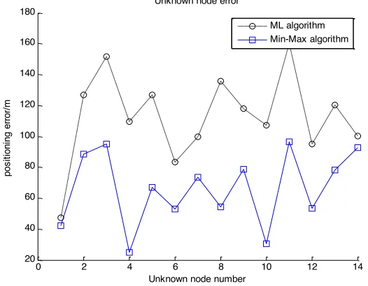
In order to verify the positioning accuracy of anchor node by using maximum size (Min-Max) and maximum likelihood estimation (ML), this two kinds of positioning algorithms are simulated and analyzed in this paper. The simulation area is set to 200 * 200, simulation 100 times to take the mean.

Assuming that the communication radius is 40m, 20 random nodes are randomly deployed in the 200 * 200 meter area. In Figure 2 and Figure 3, 15 and 6 anchor nodes are respectively deployed. The simulation uses Min-Max method and ML method to solve unknown nodes. It can be seen from these two figures that ML positioning method has higher accuracy when there are more anchor nodes, and the highest accu-racy is about 20 meters higher than Min-Max method. Min-Max positioning accuaccu-racy is higher than ML method when there are fewer anchor nodes, and the highest accura-cy is about 50 meters. It can be seen that in the case of low proportion of anchor nodes, low computational complexity and low computational load, Min-Max method is usually used, which not only reduces the communication cost, but also reduces energy consumption. When the proportion of anchor nodes is high, ML method should be used to improve the positioning accuracy. Therefore, when solving un-known node coordinates, it is necessary to select the appropriate algorithm according to the network deployment.

'

(

) / 2

i i

HS

=

HS

+

v

(

) / 2

j j

HS

=

HS

+

v

(

) / 2

k k

HS

=

HS

+

v

p

i j k

, ,

d

=

3

´

HS

d

=

2

´

HS

'

3

pk k

Fig. 2. Error comparison of two localization algorithms when the anchor node is 15

Fig. 3. Error comparison of two localization algorithms when anchor nodes are 6

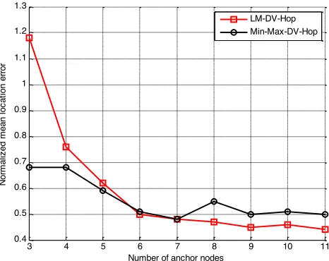
In order to further determine the relationship between the ratio of anchor node and the accuracy of the two algorithms, the normalized average positioning error of the two algorithms is simulated in Figure 4 when the number of anchor nodes is increased from 3 to 11. It can be seen from the figure that ML algorithm more dependent on the

0 2 4 6 8 10 12 14

0 20 40 60 80 100 120

Unknown node number

pos

itioni

ng er

ror

/m

Unknown node error

ML algorithm Min-Max algorithm

0 2 4 6 8 10 12 14

20 40 60 80 100 120 140 160 180

Unknown node number

pos

iti

oni

ng er

ror

/m

Unknown node error

ratio of anchor nodes. When the number of anchor nodes is small, the error of ML algorithm is large.

Fig. 4. Contrast Diagram of Two Algorithms with the Number of Anchor Nodes

Table 1. Comparison of the two algorithms of normalized average localization error

Communication radius Proportion of Anchor nodes 20% Proportion of Anchor nodes 30% ML-DV-Hop Min-Max-DV-Hop ML-DV-Hop Min-Max-DV-Hop 35 1.0520 0.9320 0.8576 0.8697 40 0.8176 0.8152 0.6641 0.6527 45 0.7158 0.6315 0.5469 0.5221 50 0.6310 0.6023 0.4432 0.4815 55 0.5178 0.5680 0.3928 0.4361

As shown in Table 1, the better the performance of Min-Max-DV-Hop algorithm is, the lower the proportion of anchor nodes is, the higher proportion of anchor nodes is, and the better performance of ML-DV-Hop algorithm is. The network area is 200*200m, and the critical proportion of anchor nodes is 30% when the total number of nodes is 20.

Iterative refinement based on Quasi Newton method: The distance between the

anchor node and the unknown node is found. Assuming that the unknown node in K anchor nodes participates in the localization, the equation set shown in (6) can be used.

When the distance between the anchor node and the unknown node is found, if there are k anchor nodes in which the unknown node p participates in, the equation (6) can be used.

3 4 5 6 7 8 9 10 11

0.4 0.5 0.6 0.7 0.8 0.9 1 1.1 1.2 1.3

Number of anchor nodes

Nor

m

al

iz

ed m

ean l

oc

at

ion er

ror

(6)

The equation (6) is transformed into a nonlinear optimization problem, namely:

(7)

Among them, the coordinates of anchor node are ; is the distance be-tween unknown node and anchor node. For the optimization problem, it needs to obtain the optimal solution of the objective

func-tion .

In this algorithm, in order to make the positioning accuracy higher and solve the objective function quickly, the estimated coordinate is set as the initial point approximation of the Quasi-Newton algorithm firstly, and is regarded as the convergence criterion of the algorithm. A new approximation point is obtained and the gradient fall of is guaranteed until the opti-mal solution is obtained by finite iteration [12].

3

Simulation and Experiment

3.1 Simulation environment and evaluation indicators

In this paper, the improved positioning algorithm is simulated by using MATLAB simulation platform, and compared with the classical improved DV-Hop algorithm in recent two years. Reference [15] is recorded as ORDV-Hop. The performance of the algorithm can be fully demonstrated by simulating and analyzing the simulation envi-ronment, topology and node characteristics of wireless sensor networks. The network topology is set as follows: 100 nodes are randomly generated in the network, and the network parameters such as the sum-up points, anchor nodes and communication radius are the same in each simulation.

CNDV-Hop algorithm is evaluated by calculating the average location error, the normalized average location error, the root mean square error by equations

， and

2 2 2

1 1 1

2 2 2

( ) ( )

( _k ) ( _k ) _k

x x y y d

x x y y d

ì - + - =

ï í

ï - + - =

î

!

2 2 2 2

1

( , ) (( ) ( ) )

min ( , ) k

i i i

i

f x y x x y y d

f x y

=

ü

= - + - - _ï

ý ï þ

å

i

( , )

x y

d

( , )

X x y* * *

,y

( , ),

f x y x R

Î

Î

R

(0) 0 0

( , )

X x y

1

(

)

f x

£

e

(1) 1 1

( , )

X x y f x y( , )

( , )

X x y* * *

1 1

N K i i j i T T

AE KN = = -=

åå

i M e i r i

3.2 Simulation analysis

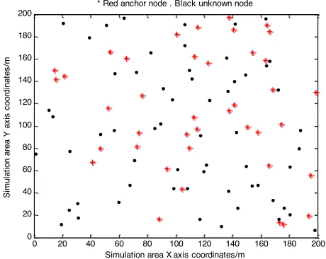
Figure 5 is the topological structure of wireless sensor networks, which is set as 200 * 200, and the area is distributed with 100 nodes randomly. Figures 6 and Figure 7 simulate the deviation between the actual and estimated positions of the unknown nodes in DV-Hop and CNDV-Hop algorithms respectively. From these two figures, it can be seen that the localization accuracy of CNDV-Hop algorithm is significantly higher than DV-Hop algorithm.

Fig. 5. Random distributions of network nodes

0 20 40 60 80 100 120 140 160 180 200

0 20 40 60 80 100 120 140 160 180

200 * Red anchor node . Black unknown node

Simulation area X axis coordinates/m

Si

m

ul

at

ion ar

ea Y

ax

is

c

oor

di

nat

es

/m

0 20 40 60 80 100 120 140 160 180 200

0 20 40 60 80 100 120 140 160 180 200

Simulation area X axis coordinates/m

Si

m

ul

at

ion ar

ea Y

ax

is

c

oor

di

nat

es

Fig. 7. Error chart for the Actual Position and Estimated Position of CNDV-Hop Algorithms

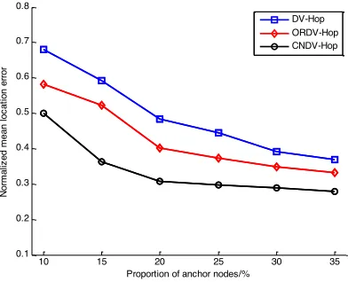
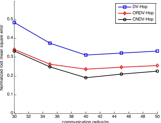
In Figure 8, it sets the ratio of anchor nodes is 30%. When R (communication radi-us) is 30 meters, the influence of the anchor node on the positioning results is simulat-ed in different proportions. It can be calculatsimulat-ed from the simulation that the normali-zation error of DV-Hop algorithm is 0.5164; the ORDV-Hop algorithm is about 0.4147 and the CNDV-Hop algorithm is 0.3829. In Figure 9, when R is 40 meters. The normalization error of DV-Hop algorithm is about 0.2958, and the ORV-Hop algorithm is about 0.2530. However, CNDV-Hop algorithm proposed in the paper is only 0.1753. In Figure 10, the proportion of anchor nodes is 30%. The simulation results show that the normalized root mean square error of CNDV-Hop algorithm is the lowest. When the communication radius is 40, the normalized root mean square error of DV-Hop algorithm is 0.3221, while the normalized root mean square error of CNDV-Hop algorithm is only 0.1765.

Fig. 8. The influence of anchor node proportion change on positioning error when R is 30

0 20 40 60 80 100 120 140 160 180 200 0

20 40 60 80 100 120 140 160 180 200

Simulation area X axis coordinates/m

Si

m

ul

at

ion ar

ea Y

ax

is

c

oor

di

nat

es

/m

10 15 20 25 30 35 0.1

0.2 0.3 0.4 0.5 0.6 0.7 0.8

Proportion of anchor nodes/%

Nor

m

al

iz

ed m

ean l

oc

at

ion er

ror

Fig. 9. The influence of anchor node proportion change on positioning error when R is 40

Figure 10 The influence of communication radius on root mean square error when the pro-portion of anchor nodes is 40%.

10 15 20 25 30 35

0.1 0.15 0.2 0.25 0.3 0.35 0.4 0.45 0.5

Proportion of anchor nodes/%

Nor

m

al

iz

ed m

ean l

oc

at

ion er

ror

DV-Hop ORDV-Hop CNDV-Hop

30 32 34 36 38 40 42 44 46 48 50 0

0.1 0.2 0.3 0.4 0.5

communication radius/m

Nor

m

al

iz

ed r

oot

m

ean s

quar

e er

ror

4

Conclusion

In this paper, a WSN localization algorithm based on DV-Hop is proposed, and the average hop distance and location calculation are corrected respectively. The im-proved average hop distance makes full use of the optimized anchor node information and has higher positioning accuracy than single anchor node. In the location calcula-tion method, the improvements of the algorithm mainly include initial value estima-tion and final estimaestima-tion of node coordinates. In the initial estimaestima-tion, when there are fewer anchor nodes, Min-Max algorithm is used to solve the problem, and ML algo-rithm is used to solve the problem when there are more anchor nodes. At this time, through simulation, the localization algorithm of the proportion of anchor nodes in different situations is given. In the final estimation, the Quasi-Newton algorithm is used to iteratively optimize the initial value. Experiments show that the algorithm is a simple and efficient ranging-free positioning algorithm for wireless sensor networks.

5

Acknowledgement

The work was supported by Projects of Natural Science Foundational in Higher Education Institutions of Anhui Province (KJ2017A449);

6

References

[1]Zhong-min Pei, Yi-bin Li, Shuo Xu. (2013). A fast localization algorithm for large-scale wireless sensor networks, Journal of China University of Mining & Technology, Vol. 42(2), pp. 314-319

[2]En-jie Ding, Xin Qiao, Fei Chang. (2014). Improved Weighted Centroid Localization Al-gorithm Based on RSSI Differential Correction, International Journal on Smart Sensing and Intelligent Systems, Vol. 7(3), pp. 1156-1173 https://doi.org/10.21307/ijssis-2017-699

[3]Capkun S, Hamdi M, Hubaux J P. (2001). GPS-free positioning in mobile Ad-Hoc net-works, Proc Hawaii International Conference on System Sciences, Maui, HW, USA, pp. 3481-3490.

[4]Doherty L, Pister K, and Ghaoui L, (2001). Convex Position Estimation in Wireless Sensor Networks, Proc. of the IEEE INFOCOM, Anchorage, AK, USA, pp. 1655-1663.

https://doi.org/10.1109/INFCOM.2001.916662

[5]Harter A, Hopper A, Steggles P, (2002). The Anatomy of a Context-Aware Application, Wireless Network, pp. 187-197. https://doi.org/10.1023/A:1013767926256

[6]He T, Huang C D, Blum B M, (2003). Range-Free Localization Schemes for Large Scale Sensor Networks, Proceedings of the Ninth Annual International Conference on Mobile Computing and Networking San Diego, United states, pp. 81-95. https://doi.org/10. 1145/938985.938995

[8]Xin Qiao, Han-Sheng Yang, Zheng-Chuang Wang, (2017). Iterative L-M Algorithm in WSN – Utilizing Modifying Average Hopping Distances, International Journal of Online Engineering, Vol. 10(13), pp. 4-20. https://doi.org/10.3991/ijoe.v13i10.7006

[9]Yan-heng Liu, Bing-ri Liu, etc, (2010). Improved DV-Hop algorithm in localization accu-racy in WSN, Journal of Jilin University (Engineering and Technology Edition), Vol. 40(3), pp. 763-768.

[10]Kai Su, Yuan Cao, etc, (2010). On hybrid localization based on UWB and DGPS, Com-puter Applications and Software, Vol. 27(5), pp. 212-215.

[11]Jin-Zhao Lin, Xiao-Bing Chen, Hai-Bo Liu, (2009). Iterative algorithm for locating nodes in WSN based on modifying average hopping distances, Journal on Communications, Vol. 30(10), pp. 107-113.

[12]Xin Qiao, Fei Chang, En-Jie Ding, (2014). Modifying Average Hopping Distances Based Iterative Algorithm for Quasi-Newton in WSN, Chinese Journal of Sensors and Actuators, Vol. 27(6), pp. 797-801.

[13]Wei-Wei JI, Zhong Liu. (2008). Study on the application of DV-Hop localization algo-rithms to random sensor networks, Journal of Electronics& Information Technology, 30(4):970-974.

[14]Xin Qiao, (2015). Localization Algorithm of Wireless Sensor Network and Its Improve-ment Based on DV-Hop, China University of Mining and Technology, Xuzhou.

[15]Yu-Cheng Wu, Jiang-Wen Li, (2012). Improved DV-Hop Localization Algorithm Based on Optimal Communication Radius of Nodes, Journal of South China University of Tech-nology (Natural Science Edition), Vol. 40(6), pp. 36-42.

7

Authors

Ms. Xin-Qiao, was born in 1988, Suzhou City, Anhui Province, China. She is a

Lecturer and having a Master’s degree. She has been published a number of high-level papers and her research interests are wireless sensor network positioning tech-nology, ZigBee technology etc. She is with School of Electronic Engineering, Chaohu University, Chaohu, 238000, Anhui, China.

Fei-Chang is with Inspur Group Company Limited, Jinan, 250000, Shandong,

China.

Jing--Ling is with School of Electronic Engineering, Chaohu University, Chaohu,

238000, Anhui, China.