A New Model for Software Reliability Evaluation Based on NHPP with Imperfect Debugging

(1)

8thSASTech 2014Symposium on Advances in Science & Technology-Commission-IV Mashhad, Iran

A New Model for Software Reliability Evaluation Based on

NHPP with Imperfect Debugging

Shiva Akhtarian

MSc Student, Department of Computer Engineering and Information Technology, Payame Noor University, Iran

[email protected]

TahereYaghoobi

Assistant Professor, Department of Computer Engineering and Information Technology Payame Noor University, Iran

[email protected]

Abstract — In new software products, the necessity of high reliability software development is increasingly important to all software developers and customers. Software reliability modeling based on Non Homogenous Poisson Process (NHPP) is one of the successful methods in predicting software reliability. One of the most important assumptions in modeling software reliability is imperfect phenomenon which describes the probability of introducing new faults to the software during debugging process. In this paper a new imperfect model is proposed by considering complexity and dependency between faults. Estimating the model parameters has been done by using failure data sets of four real software projects through MATLAB software. Comparison of the proposed model is done with two existing models using various criteria. The results show that the proposed model better fits the real data and then providing more accurate information about the software quality.

Keywords — Software Reliability, Non Homogenous Poisson Process, simple and complex faults, dependency, time delay, imperfect debugging

1. I

NTRODUCTION

An important approach in evaluating software quality and performance is to determine the software reliability. Software reliability defined as the probability of error free software operation in a specified environment for a specified time (Yamada, 2014). In the last three decades various software reliability growth models (SRGMs)1 have been developed. Most of the SRGMs based on NHPP present the reliability diagram as concave or S-shaped curve (Goel, 1985; Pham, 2006; Kapur, et al., 2011; Lai, et al., 2012). If the reliability is uniformly growth, concave models are used otherwise it would be S-shaped. In 1985 Goel and Okumoto proposed a concave model which assumed that total faults in the software are independent and probability of detecting faults in a unit of time is constant (Goel, 1985). They also assumed detected faults are immediately removed and no new faults are introduced during debugging (perfect debugging). In an S-shaped model detected faults are

1

Software Reliability Growth Model

immediately removed and perfect debugging is used but fault detection rate is time dependent (Yamada, et al., 1983; Yamada, et al., 1984; Yamada, et al., 1985). In lots of recent researches imperfect debugging is considered in modeling, which shows the probability of introducing new faults to the software during fault correction and removal (Yamada, et al., 1992; Pham, 2006; Pham, 2007; Gaggarwal, et al., 2011; Gupta, et al., 2011).

In some of developed models detected faults are categorized according to their dependency or complexity. Ohba proposed the idea of fault dependency in 1984 by assuming that independent faults can be removed immediately after they are detected but dependent faults cannot be removed until their leading faults are eliminated (Ohba, 1984). Kapour and Younes in 1995 affected fault dependency into G-O model (Kapur, et al., 1995). They noticed that time delay effect factor between detecting and removing dependent faults is negligible. In studies by Hung and Lin dependent and independent faults are modeled based on NHPP with some various times dependent delay functions (Huang, et al., 2004; Huang, et al., 2006).

Karee and his colleagues proposed an S-shaped model with fault complexity by categorizing faults as simple and hard. In their model simple faults can be removed immediately but they affected two steps of observing and removing to eliminate hard faults (Kareer, et al., 1990). Kapur In 1999 developed a model by considering software testing as a three step process, including observing, isolating and removing faults. Based on this assumption, he proposed a model with three types of faults categorized based on their complexity. In which simple faults can be removed immediately after they are detected, hard faults are those that need a time delay factor between observing and isolating the fault and complex faults need a time delay effect factor between observing, isolating and removing the fault (Kapur, et al., 1999).

(2)

presented based on some assumptions.

In software reliability modeling there are unknown parameters that can be determined by Maximum Likelihood Estimation (MLE) or least squared estimation methods (Zacks, 1992; Pham, 2006). The unknown parameters of the proposed model are determined by using four real software fault data sets by MLE. Then some of statistical criteria are used to compare the goodness of fit of the new model and two basic models. The estimated time to stop testing for software is evaluated by the proposed model.

The remainder of paper is as follows: In Section 2, a generic NHPP software reliability model is explained. Section 3 is dedicated to one application of software reliability estimation, estimating time to stop software testing. In Section 4, the parameters, assumptions and our modeling is described in details. The next two sections, 5 and 6are specified to model estimation, and model validation respectively. The paper is concluded in Section 7.

2. S

OFTWARE RELIABILITY

M

ODELING BASED

ON

NHPP

The basic assumption in NHPP modeling is that the failure process is described by the NHPP.

Most of software reliability growth models follow the general assumptions regarding the fault detection process which can be considered as follows.

Detecting / removing faults are modeled by NHPP. All faults are independent from each other and they are equally recognizable.

The number of faults detected at any time is proper with the number of remaining faults in the software. Each time a failure occurs an error that led to it is immediately and completely removed and no new errors introduced in the meantime (perfect debugging).

Assume that N(t) is the number of detected errors (failures observed) at time t and m(t) is the mean number of detected faults until time t, then its Min Value Function (MVF) is:

n m t m t

Pr N t n e n 0,1, 2,

n !

(1)

Where

0

t

m t s ds and is failure intensity

function (number of failures per unit of time). dm t

λ t

dt (2) Therefore, the overall reliability model based on NHPP is

obtained by solving the following differential equation with the initial condition m (0) =0:

dm t

λ t b t . a m t

dt (3)

In which, "a" represents the total number of initial faults in the software before testing. Expression [a–m(t)] shows

the mean number of remaining faults in the software at time t, and b(t) is fault detection rate.

General solution for the differential equation 3 is as follows:

β t β t

m t e [C ab t e dt](4)

In which:

β t b t dt

And C is the constant of integration.

Finally the software reliability is achieved through the following formula:

t

0 λ s ds

R t

e

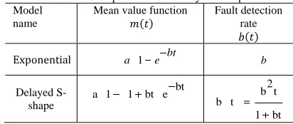
(5)

Table1 [3] shows details of two basic models for software reliability, Goel - Okumoto exponential model and delayed S-shaped model.

Table 1. Details of exponential and delayed s-shape models Model

name

Mean value function Fault detection rate

1 bt

a e b

Delayed S-shape

bt

a 1 1 bt e b t2

b t 1 bt

3. E

STIMATING

T

IME TO

S

TOP

S

OFTWARE

T

ESTING

Software testing is a costly process, so it's necessary to terminate it in a suitable time. One of the applications of estimating software reliability is to determine the appropriate time to terminate software testing.If the software reached to an acceptable level of reliability at the specified time, then decision to terminating the test can be taken. To achieve this goal, the conditional reliability function, R x t| is used. This function assumes that the last failure has occurred at time t and no new failure happens at time interval t t, x Therefore (Pham, 2006):

| 0 m t x m t

R x t Pr N t x N t e (6)

4.T

HE

P

ROPOSED

M

ODEL

In this section, first the model parameters and assumptions are presented and then, according to the provided assumptions, the modeling is carried out.

4.1.PARAMETERS OF THE PROPOSED MODEL

a : total number of initial faults in the software.

1

a ,a2,a3: total number of initial simple, independent

complex, dependent complex faults.

1 2 3

b , b , b : fault detection rate for Simple, independent complex, dependent complex faults

1 2 3

α , α , α : fault introduction rate for simple, independent complex, dependent complex faults.

(3)

: proportion of independent complex and dependent complex.

1

φ t : time lag for complex independent faults.

2

φ t : time lag for complex dependent faults.

m t : mean value function for total software faults.

1

m t : mean value function for simple faults.

2 1

m t φ t mean value function for independent complex faults.

3 2

m t φ t : mean value function for the dependent complex faults.

4.2.ASSUMPTIONS OFTHE PROPOSED MODEL

Our proposed model assumptions are as follows: i. Detecting / removing faults is modelled by NHPP. ii. Software faults are divided into simple and complex

faults. This division was done by considering the amount of effort needed to remove them.

iii. Simple faults can be corrected and deleted immediately after detection.

iv. Complex faults may need more effort to be removed. This kind of fault is considered in dependent and independent.

v. Independent complex faults need more times than simple faults to be removed. Therefore the time delay factor

φ t

1 is affected to show the amount of

efforts is needed for this type of faults.

vi. Dependent complex faults arise due to the presence of an independent complex fault. This kind of fault cannot be removed unless its leading fault is eliminated. According to the effort required in removing this type of fault, time delay factor is not negligible, therefore the latency

φ t

₂ will be

affected

vii. During the debugging process, introducing new faults is possible to show the imperfect phenomenon.

4.3.MODELING

The total number of detected faults during the time (0, t) is equal to

(7)

1 2 1 3 2

m t = m t + m t - φ t + m t - φ t

Let a be the total number of initial faults before testing and a1,a2,a3 describe total number of initial simple,

independent complex and dependent complex faults respectively. So we have:

1

a = pa a = 1 - p qa₂ a = 1 - p₃ 1 - q a

Detection and removal process of simple faults follows the general reliability modeling (Equation 3) with constant fault detection rate.

Of course time lag to remove faults is negligible and imperfect debugging is affected by new faults introduced to software during debugging as shown in equation (8):

1

1 1 1 1 1

dm t

= b a + α m t - m t

dt

(8)

By solving the differential equation (8), the mean value function of the detected faults is created as follows

1 1 1 1

-b t 1-α -b t 1-α

1 1

a pa

m t = 1 - e = 1 - e

1 - α 1- α (9)

Software debugging team requires more time to discover the causes of complex faults to remove them. For this type of faults general model of reliability can be used, however it is necessary to affect time delay factor and imperfect debugging in removal process.

Assuming that the mean value function of the independent complex faults is proportional to the remaining number of independent complex faults and new faults introduced to the system, so:

2

2 2 2 2 2

dm t

= b a + α m t - m t dt

(10)

By solving the differential equation (10), in initial condition m2 0

0

will have:

2 2 -b t 1-α 2

2

a m t = 1 - e

1 - α

2 2

-b t 1-α

2

1- p qa

= 1- e

1- α (11)

Time delay factor in debugging of independent complex faults is considered as ascending functionφ t . Thus 1

the finalequation (12) is obtained:

Ln 1 + b t 2 φ t =

1

b 2

2 2 2 1-α -b t 1-α

2 1 2

2 1 - p qa

m t - φ t = 1- 1+ b t e

1 - α (12)

Based on assumption v, the general modeling of reliability is not directly applicable on removing dependent complex faults.

The mean value of dependent complex faults is proportional to the number of remaining dependent complex faults, the mean value of independent complex faults and new introduced faults to the system. Also, time delay factor φ₂ t and imperfect debugging are

affected to remove this kind of faults. So the differential equation for modeling these faults is as follows:

3 2 1

3 3 3 3 3

2 3

dm t m t - φ t

= b a + α m t - m t

dt a + a

(13)

By solving equation (13), we obtain

3 3

3 a

m t = ×

1 - α (14)

2 2 2

2

1 1 2 3 3

2 0

2 3 2 3

1

1 exp (1

1

) 1

1

t

b s

a b s

b s e ds

a a b s

(4)

equation of complex dependent faults. So we have:

3 Ln 1 + b t φ_{2 t} =

b3

3 2

m t - φ t = (15)

2 ₂

1 1 2 1

3 2 3 3 2 2

1 exp (1 1

2

1 1 ₀ 1

3 2 3 2 3

t t

a a b s _{b s}

b s e ds

a a b s

According to equation (7), the mean value function of total software’s faults is obtained by calculating all three mean value functions.

5. M

ODEL ESTIMATION

The proposed model is tested on four real software failure data sets, real-time command and control system (Ohba, 1984a), IBM (Musa, et al., 1987), OCS (Pham, et al., 2003) and Misra (Misra, 1983) and its parameters are estimated by Matlab2012 software. Table (2) presents estimated parameters for the proposed model, exponential model and delayed S-shaped model.

Table2.Parameter estimation based on failure datasets

Real time IBM OCS Misra Model name ˆ 150 a

ˆ _{0 / 5} 1

b

ˆ _{0 / 13} 2

b

0 / 01 3

ˆ ₀₀

b

ˆ 0 / 42

s

ˆ 0 / 94

q

ˆ₁ 0 / 03

0 / 01 2

ˆ 00

ˆ₃ 0 / 85 ˆ 71

a

ˆ _{0 / 03} 1

b

ˆ _{0 / 09} 2

b

ˆ _{0 / 99} 3

b

ˆ 0 / 43

s

ˆ 0 / 56

q

0 / 01 1

ˆ 00

0 01 2

ˆ / 0

0 01 3

ˆ / 0

ˆ 380

a

ˆ _{0 / 18} 1

b

ˆ _{0 / 19} 2

b

0 / 01 3

ˆ ₀₀

b

ˆ 0 / 17

s

ˆ 0 / 34

q

0 / 01 1

ˆ 00

0 / 01 2

ˆ 00

0 01 3

ˆ / 0

ˆ 378

a

ˆ _{0 / 69} 1

b

ˆ _{0 / 16} 2

b

ˆ _{0 / 09} 3

b

ˆ 0 / 06

s

ˆ 0 / 21

q

ˆ₁ 0 / 06

ˆ₂ 0 / 54

ˆ₃ 0 / 99

New model

ˆ 142

a

ˆ _{0 / 12}

b

ˆ 400

a

ˆ _{0 / 005}

b

ˆ 242

a

ˆ _{0 / 06}

b

ˆ 922

a

ˆ 0 / 007

b G-O model

ˆ 136

a

ˆ _{0 / 28}

b

ˆ 71

a

ˆ _{0 / 1}

b

ˆ 153

a

ˆ _{0 / 31}

b

ˆ 285

a

ˆ _{0 / 08}

b

Delayed

S-shaped model

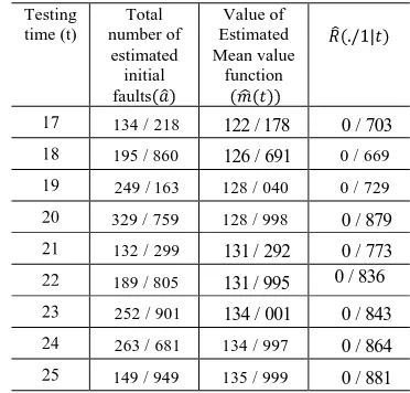
Now using obtained parameters, mean value function and software reliability can be estimated in a time interval

, 0.1

t t . Thus, the time termination of software testing is specified. Table (3) presents the information of software testing process obtained by using proposed model on real-time command and control system from

time 17 to 25 to estimate the software testing time termination.

Table Obtained information after each test of real-time command and control system to determine the terminating time of testing process

using proposed model

Value of Estimated Mean value function Total number of estimated initial faults Testing time (t)

0 / 703 122 / 178

134 / 218

0 / 669 126 / 691

195 / 860

0 / 729

128 / 040

249 / 163

0 / 879

128 / 998

329 / 759

0 / 773 131 / 292

132 / 299

0 / 836 131 / 995

189 / 805

0 / 843 134 / 001

252 / 901

0 / 864

134 / 997

263 / 681

0 / 881

135 / 999

149 / 949

6. M

ODEL

V

ALIDATION

To show the validation of the proposed model assumptions, we compare it with exponential model and delayed S-shaped model which are considered as basic models in predicting software reliability, based on NHPP. Figures (1) to (4) shows the proposed model's goodness of fit compared with the exponential model and delay S-shaped model on all four data sets mentioned in the last section.

Figure1.proposed model's goodness of fit compared with, Exponential model and delay S- shaped model on real time command and control

dataset

(5)

Figure 3.proposed model's goodness of fit compared with, Exponential model and delay S- shaped model on OCS dataset

Figure 4.proposed model's goodness of fit compared with, Exponential model and delay S- shaped model on Misra dataset

It can be seen from figures, the proposed model is properly consistent on data sets.

For accurate model comparison, other criteria can be used. Three common ones are PRR1 (Pham, et al., 2003), SSE2 (Pham, 2006) and MSE3 (Pham, 2006), which can be expressed as follows:

"y" is total number of faults observed at time "t" according to real dataset and "m(t)" is estimated cumulative number of faults at time "t" and "n" is the number of observations.

In model comparison, smaller values for each of three criteria on the same dataset, represents more appropriate model.

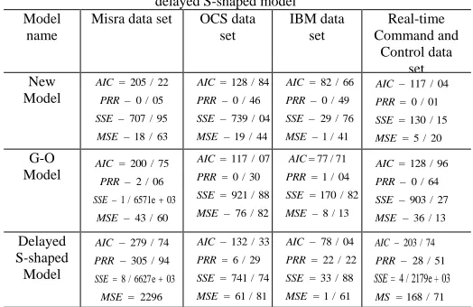
Table (4) shows the obtained values of criteria for proposed model, exponential model and delayed S-shaped model on all four datasets.

1_{Prediction Ratio Risk} 2

Sum of Squared Errors

3_M

ean Squared Errors

Table3.values of criteria for proposed model, exponential model and delayed S-shaped model

Real-time Command and

Control data set IBM data

set OCS data

set Misra data set

Model name

117 / 04 AIC

0 / 01 PRR

130 / 15 SSE

5 / 20 MSE 82 / 66 AIC

0 / 49 PRR

29 / 76 SSE

1 / 41 MSE 128 / 84 AIC

0 / 46 PRR

739 / 04 SSE

19 / 44 MSE 205 / 22 AIC

0 / 05 PRR

707 / 95 SSE

18 / 63 MSE New Model

128 / 96 AIC

0 / 64 PRR

903 / 27 SSE

36 / 13 MSE 77 / 71 AIC

1 / 04 PRR

170 / 82 SSE

8 / 13 MSE 117 / 07 AIC

0 / 30 PRR

921 / 88 SSE

76 / 82 MSE 200 / 75 AIC

2 / 06 PRR

1 / 6571e 03 SSE

43 / 60 MSE G-O Model

203 / 74 AIC

28 / 51 PRR

4 / 2179e 03 SSE

168 / 71 MS 78 / 04 AIC

22 / 22 PRR

33 / 88 SSE

1 / 61 MSE 132 / 33 AIC

6 / 29 PRR

741 / 74 SSE

61 / 81 MSE 279 / 74 AIC

305 / 94 PRR

8 / 6627e 03 SSE

2296 MSE Delayed S-shaped Model

According to the results of Table 4,it can be seen thatthe proposed model has a good fitness on mentioned datasets and works better than the exponential model and delayed S-shaped model.

7. C

ONCLUSION

Software reliability growth models can be used to determine software performance and control the testing process of software.

Based on these models, reliability is estimated in quantitative methods. Some measurements such as number of initial faults, failure intensity, software reliability in a specified period of timeand mean time between failures can be determined by using SRGMs. By now, various models have been developed by researchers based on software testing conditions.

New software reliability model proposed in this paper, categorizes software faults into simple, independent complex and dependent complex. The model is also affected by imperfect debugging and time delay factor in complex faults removal modelling.

By considering new assumptions more realistic model proposed, which considers both complexity and dependency of faults in its fault removal modelling. Imperfect debugging and time delay factor in removing complex faults are two other important assumptions in new model. So by making this model more closer to real software conditions it can estimate software reliability more accurate than compared basic models.

R

EFERENCE

[1] S. Yamada, Software reliability modeling: Fundamentals and Applications.: Springer, 2014. [2] A. L. Goel, "Software Reliability

Models:Assumptions, Limitations and applicability," IEEE Trans.on software engineering, vol. 11, pp. 1411-1423, 1985.

[3] H. Pham, System Software Reliability. London: Springer-Verlag, 2006.

(6)

Software Reliability Models," Journal of Software, vol. 7, pp. 1296-1306, 2012.

[6] S. Yamada, M. Ohba, and S. Osaki, "S-shaped Reliability Growth Modeling for Software Error Detection," IEEE Trans on Reliability, vol. 32, no. 5, pp. 475-484, 1983.

[7] S. Yamada, M. Ohba, and S. Osaki, "S-shaped Software Reliability Growth Models and their Applications," IEEE Trans.Reliability, vol. R-33, pp. 289-292, 1984.

[8] S. Yamada and S. Osaki, "Software reliability growth modeling: models and applications," IEEE Trans Softw Eng, pp. 1431-1437, 1985.

[9] S. Yamada, K. Tokunou, and S. Osaki, "S-Imperfect debugging models with fault introduction rate for software reliability assessment," International Journal of Science, vol. 23, no. 12, pp. 2241-2252, 1992.

[10] H. Pham, "An imperfect-debugging fault detection dependent parameter software," International Journal of Automation and computing, pp. 325-328, 2007.

[11] A. Gaggarwal, P. K. Kapur, and A. S. Garmabaki, "Imperfect Debugging software reliability growth model for multiple release," in 5th national conference, India, 2011.

[12] A. Gupta and S. Saxena, "Software Reliability Estimation Using Yamada delayed S Sape Model under Imperfect Debugging and Time Lag," in International Coference on Advanced Computing & Communication technologies, vol. 5, 2011, pp. 317-319.

[13] M. Ohba, "Software Reliability Analysis Models," IBM Journal of Research and Development, vol. 28, pp. 428-443, 1984.

[14] P. K. Kapur and S. Younes, "Software Reliability Growth Model with error dependency," Elsevier Science, vol. 35, pp. 273-278, 1995.

[15] C. Y. Huang, C. T. Lin, J. H. Lo, and C. C. Sue, "Effect of Fault Dependency and Debugging Time Lag on Software Error Models," IEEE Trans on Reliability, pp. 243-246, 2004.

[16] C. Y. Huang and C. T. Lin, "Software Reliability Analysis by Considering Fault Dependency and Debugging time Lag," IEEE Trans on Reliability, vol. 55, pp. 436-450, 2006.

[17] N. Kareer, P. K. Kapur, and P. S. Grover, "An S-shaped software reliability growth model with two types of errors," Microelectron Reliab, pp. 1085-1090, 1990.

[18] P. K. Kapur, R. B. Garg, and S. Kumar, Contributions to hardware and software reliability. Singapore: Word Scientific, 1999.

[19] S. Zacks, Introduction to Reliability Analysis.: Springer-Verlag, 1992.

[20] M Ohba, Software reliability analysis models.: IBM Development, 1984a.

[21] J D Musa, A Lannino, and K Okumoto, Software Reliability: Measurement, prediction, and application. New York: Mac Graw-Hill, 1987.

[22] H Pham and C Deng, "Predictive ratio risk criterion for selecting software reliability models," in Ninth International Conf on reliability and quality in design, 2003.

[23] P. N. Misra, "Software reliability analysis," IBM System Journal, pp. 262-270, 1983.