Continuous Time Markov Chain Models of Voltage Gating of Gap
Junction Channels
Henrikas Pranevicius
Department of Applied Informatics, Vytautas Magnus University,
Department of Business Informatics Research in Systems, Kaunas University of Technology, Studentų St. 56, LT – 51424 Kaunas, Lithuania,
e-mail: [email protected]
Mindaugas Pranevicius
Department of Anestesiology, Albert Einstein College of Medicine, 1300 Morris Park Ave., Bronx, NY 10461, USA,
e-mail: [email protected]
Osvaldas Pranevicius
Department of Anestesiology, New York Hospital Queens, 56-45 Main Street, Flushing, NY 11355, USA,
e-mail: [email protected]
Mindaugas Snipas
Department of Business Informatics Research in Systems and
Department of Mathematical Research in Systems, Kaunas University of Technology Studentų St. 50, LT – 51368 Kaunas, Lithuania
e-mail: [email protected]
Nerijus Paulauskas
Institute of Cardiology, Lithuanian University of Health Sciences, Department of Business Informatics, Kaunas University of Technology,
Studentų St. 56, LT – 51424 Kaunas, Lithuania, e-mail: [email protected]
Feliksas Bukauskas
Department of Neuroscience, Albert Einstein College of Medicine, 1300 Morris Park Ave., Bronx, NY 10461, USA,
e-mail: [email protected]
Abstract. The major goal of this study was to create a continuous time Markov chain (CTMC) models of voltage gating of gap junction (GJ) channels formed of connexin protein. This goal was achieved by using the Piece Linear Aggregate (PLA) formalism to describe the function of GJs and transforming PLA into Markov process. Infinitesimal generator of CTMC was used to automate construction of Markov chain model from description of the system using PLA formalism. Developed Markov chain models were used to simulate gap junctional conductance dependence on transjunctional voltage. The proposed method was implemented to create models of voltage gating of GJ channels containing 4 and 12 gates. CTMC modeling results were compared with the results obtained using a discrete time Markov chain (DTMC) model. It was shown that CTMC modeling requires less CPU time than an analogous DTMC model.
Keywords: Continuous time Markov chain; PLA formalism; gap junction channel; steady-state probabilities.
1. Introduction
Connexins (Cxs) is large family of integral membrane proteins that provide a direct pathway for electrical and metabolic signaling between cells [2]. 21 Cx isoforms in humans [14] form gap junction (GJ) channels. Each GJ channel is composed of two hemichannels (HCs), each oligomerized of six Cxs. Cxs have four alpha helical transmembrane domains (M1 to M4), intracellular N- and C-termini (NT and CT), two extracellular loops (E1 and E2), and a cytoplasmic loop (CL) [15]. Docking of HCs from neighboring cells leads to formation of the GJ channels composed of 12 Cxs.
Sensitivity to transjunctional voltage (Vj), called
voltage-gating, appears to be common to all GJ channels. Symmetric reductions in junctional
conductance (gj) for either polarity of Vj have been
explained by the presence of a Vj-sensitive gate in
each apposed hemichannel [1]. Gap-junctional communication plays important roles in many processes, such as impulse propagation in the heart, communication between neurons and glia, metabolic exchange between cells in the lens lacking blood circulation, organ formation during development, and regulation of cell proliferation.
Earlier, we developed stochastic 4- and 16-state models of voltage gating, containing 2 and 4 gates in series in each GJ channel, respectively. These models contain a certain number (>10) of parameters and to estimate them global optimization (GO) algorithms should be used [4]. Typically, thousands of iterations should be used in performing GO to estimate a global minimum. If a single iteration of the model lasts up to 10 s, then a search for a global minimum can take several hours or days. Thus, the reduction of computation time necessary to perform a single simulation is an important task.
Preliminary studies showed [6] that modeling of GJ channels gating using the Markov chain formalism requires over 100 – fold less CPU time than a simulation using DTMC model [5,13] describing the GJ channel containing 12 gates. In this model, differently from 4- and 16-state models, it is assumed that each connexin protein of GJ channel contain the gate. Since all 12 gates operate at the same time, construction of the transition matrix is not a trivial
task. Therefore, transition matrix P is dense, and the
run-time complexity of calculation of steady-state
probabilities is O
n3 if direct methods, i.e. Gaussianelimination, are applied.
In this study, we use CTMC, instead of DTMC, to model gating of GJ channels. The CTMC model has an advantage over DTMC, because construction of infinitesimal generator (transition rates matrix) is relatively easy, since no more than a few transitions can happen at any state of an infinitesimal time period. Moreover, the run-time complexity of a steady-state solution is significantly lower than with DTMC, since
the infinitesimal generator matrix Q is sparse. In some
cases, matrix Q is tridiagonal, which allows achieving
run-time complexity in the order of O
n to calculatesteady state probabilities.
We used Piece Linear Aggregate formalism
(PLA) [11, 12] in order to describe system behavior and to create an infinitesimal generator matrix of CTMC model of the GJ channel. Formal specification can be applied for verification of liveness of CTMC model, using special tools, e.g., Simple Promela
Interpreter (SPIN) model checker [3, 8, 9].
PLA, in essence, is equivalent to piece-linear Markov process. If duration of operations used in PLA specifications are distributed by exponential law, then the piece-linear Markov process becomes a linear CTMC process with a discrete set of states. These presumptions allow transforming a PLA specification to the specification of Markov processes and the automatic creation of a state-space graph of the analyzed system.
As reported earlier [7], automated creation of an infinitesimal generator matrix can be achieved in the following steps: 1) formal specification of the system, 2) creation of state-space graph, and 3) state-space graph transformation into the infinitesimal generator matrix. PLA formalism and its theoretical background are presented in Section 2. CTMC models of GJ channels are presented in Section 3. We also present formal specification of CTMC models using PLA formalism.
2. PLA formalism for creation of continuous
time Markov chain models
presented. We also define necessary conditions allowing transformation of PLA model into CTMC.
2.1. PLA formalism
Using the aggregate approach, the system can be represented as a set of interacting PLAs. The PLA is
characterized by a set of states zZ, input signals
X
x , and output signals
y
Y
, which varies over aset of time moments tT . To describe proper
changes of PLA properties over time, transition H and output G operators must be known.
The state zZof the PLA is the same as the state
of a piece-linear Markov process, i.e. z
t
t,z t
,where
t is a discrete state component taking valueson a countable set of values, and
z
t
is a continuouscomponent comprising of z1
t,z2 t,,zk
tcoordinates.
When there are no inputs, the state of the aggregate changes in the following manner:
t const ,
dt t
dz , (1)
where
1,2,,k
is a constant vector.The state of the aggregate can change when an input signal arrives or when a continuous component acquires a definite value.
Controlling sequence approach permits to define the continuous coordinates of PLA as follows:
tm
w
e1,tm
,we2,tm
, ,w
ef,tm
;z (2)
where
w
e
i
,
t
m
is the time moment in which the eventi
e
occurs.When the state of the system is known (z
tm ,m = 0, 1, 2, …), then the moment, tm1 , is
determined by an input signal arrival or by the following equation:
i m
m we t
t 1=min , , 1i f . (3)
The class of the next event, em1, is determined by
an input signal if it arrives at the time moment tm1 or
by the control coordinate, which acquires minimal
value at the moment
t
m, i.e. if w
ei,tm
acquiresminimal value, then em1ei.
The operator H conditions the new state:
tm H
z
tm ei
z 1 , , eiEE. (4)
The output signal
y
i from the set of output signals( Y
y1,y2,,ym
) can be generated by anaggregate only at moments of events from the subsets of internal and external events – E’ and E’’,
respectively. The operator G determines the content of
the output signals:
ztm ei
G
y , , eiE'E'', yY. (5)
PLA can be changed to Markov process with continuous time discrete state if durations of operations are distributed according to exponential law
i
tj i
i e t P t
F
1 , (6)where
i
1 is an average duration of the ith operation,
k is the number of active operations at the state z(t).
Probability, that an event will occur at system state z(t), is equal to
kk
t m
m t t e
t P
1
1 . (7)
Then, it follows that
t
t w
e t w
e t
z ; , , , f,
" "
1
, (8)
here
t is the discrete component of the state, and
e t w i,'' is defined as follows:
. otherwise ,
0
; moment at active is operation the
if , ,
'' ith t
t e
w i
i
(9)
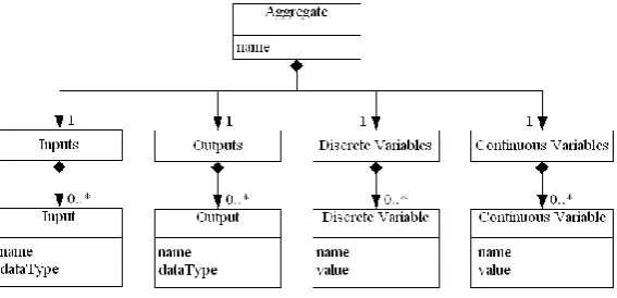
Meta-model of PLA formalism is presented below and is described using the UML notation as reported in [10].
The class diagram is demonstrated in Fig. 1. It includes inputs, outputs as well as discrete and continuous variables of an aggregate.
Continuous variables are used to describe moments during which the internal events occur after operations terminate.
Input signals cause external events.
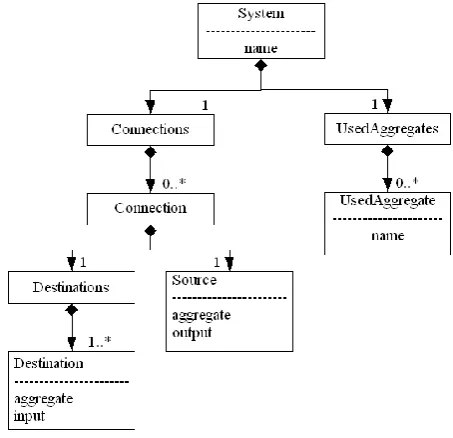
The modeling system consists of interconnected aggregates as shown in Fig. 2.
Figure 2. The system of aggregates interacting throughout shown connections
Fig. 3 shows the structure of input and output signals’ data.
Figure 3. The structure of input and output signals
2.2. Generation of state graph of CTMC
The main concept for generation of open and
closed states of gates from PLA, referred as a state
graph, is based on the fact that the subset of internal events, initiating transition among states, is known in every state.
The states graph of CTMC is described as
Z,
G , where Z is a set of system states and is a
set of transition rates (
0
:Z Z ) .
The generation of the Markov chain graph involves the following steps:
1. Collection of information about:
1.1. The set of internal events E.
1.2. The initial state of the system z(0).
1.3. The set of generated states of the system Zg,
which initially has only one member, z(0),
i.e., Zg
z
0 .1.4. The set of analyzed states Za, which initially
is empty, i.e., Za .
2. The search of neighboring states:
2.1. Choose a non-analyzed state zZg\Za
2.2. Search for eE|
e,t 0 , which canoccur in the state z:
2.2.1. Generate the set of states Z into
which the system can pass in a single step:
| , , : 0
i i i e we
e z H z z
Z ;
2.2.2.
z
Z
:2.2.2.1. Add zto Za, i.e.,
z Z Za: a
2.2.2.2. Add the new transition rate from
state z to z, i.e., :
w
ei
.3. Testing criteria defining termination of the
algorithm: ZaZg.
3. The model of the GJ channel containing 12
connexins
for different values of Vjs and obtained data compared
with results acquired using DTMC model [13].
3.1. Conceptual model of the GJ channel containing 12 connexins
Gap junctions form clusters (junctional plaques) of individual channels arranged in parallel in the junctional membrane of two adjacent cells. The GJ channel is composed of 2 hemichannels (left and right) arranged in series. Each hemichannel is composed/oligomerized from six Cxs forming a hexamer with the pore inside. We envision that each hemichannel forms the gate, which is composed of six subgates arranged in parallel, i.e. to each connexin the subgate is attributed and the GJ channel contains two gates and 12 subgates. Each subgate operates between
open (o) and closed (c) states. For simplicity, we
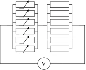
assume that only subgates in the left hemichannel operate [4], while subgates in the right hemichannel are always open (see Fig. 4).
V
Figure 4. Electrical scheme of the GJ channel composed of two hemichannels each formed of 6 connexins. Transjunctional voltage (Vj) controls both hemichannels
from which only Cxs in the left hemichannel operate between open and closed states, while Cxs in the right
hemichannel are always open
The GJ channel gates in response to Vj by
performing o↔c transitions for each subgate. Each
subgate has a possibility for four transitions as shown in Fig. 5:
O C
oc p
co p oo
p
cc p
Figure 5 The graph illustrating open (o) and closed (c) states of the gate and probabilities of transitions
As reported earlier [5], probabilities of shown transitions can be described as follows:
) , , , ( 1
) , , , ( ) , , , (
0 0 0
V V P A k
V V P A k K V V P A p
left left oc left
, (10)
) , , , ( 1 ) , , ,
(APV V0 p APV V0
poo left oc left , (11)
) , , , ( 1 ) , , , (
0 0
V V P A k
K V
V P A p
left left
co , (12)
) , , , ( 1 ) , , ,
(APV V0 p APV V0
pcc left co left . (13)
In (10) and (12), k is
) 0
0 (
) , ,
(PV V eA PVleft V k left
, (14)
where P is a gating polarity (+1 or -1); A is a
coefficient characterizing gating sensitivity to voltage
(1/mV); K is a constant used to change kinetics of
c↔o transitions (K can accelerate or decelerate c↔o
transitions but does not affect conditions of the steady
state); Vo is a voltage across the
hemichannel/connexin at which probabilities for o and
c states are equal (mV); Vleft is variable voltage
across the subgate (mV).
Each subgate, depending on a voltage across it (Vleft/right), can gate by changing stepwise between the
open state with conductance go and the closed state
with conductance gc. It was assumed that go and gc
values rectify, i.e., depend on Vleft/right exponentially:
Ro V
o right
left o
right left V P
e g P V
g
/
0 , / , )
(
,
C left
R V P V c left
c V P g e
g
, 0
) ,
( , (15)
where Vleft/right is a voltage across the left or right
hemichannel, go,V=0 and gc,V=0 are conductances at
right left
V / =0, and Ro and Rc are rectification
constants.
The conductance of the left hemichannel, when n
Cxs are closed, can be described as follows
n n g
V
n P
n
g
V
n P
gleft c left , 6 o left , . (16)
Similarly, the conductance of the right hemichannel is
n g
V
n P
gright 6 o left , . (17)
During gating, conductances of subgates range
between go(Vleft/right,P) and gc(Vleft,P) , and the total
conductance of the GJ channel can be found using steady-state probabilities of Markov chain model of the left hemichannel (see the section 3.2):
6
0
n left n
left g n
g , (18)
where n is a steady-state probability for n Cxs in
the left hemichannel to be closed.
3.2. CTMC model of the GJ channel containing 12 connexins
In order to create a CTMC model of GJ, we use the following relation in describing probabilities and rates of subgate’s transitions (see Fig. 6):
oc òc p and co co p
, (19)
where τ is a short period of time, in which the
probability to observe multiple transitions is
negligible, i.e. for i j, pij
0 if 0.O C
oc
co
Figure 6. The graph illustrating open (o) and closed (c) states of a gate with transition rates
Assuming a CTMC model allows using PLA formalism for automatic model creation, an aggregate specification of the continuous time Markov chain model of GJ channel is presented below.
1. The set of input signals: X = Ø. 2. The set of output signals: Y = Ø. 3. The set of external events: E' = Ø. 4. The set of internal events:
"2 " 1,
" e e
E ,
where "
1
e is a transition from the closed to the open
state of the subgate in the left hemichannel; "
2
e is a
transition of the subgate in the left hemichannel from the open to the closed state.
5. The transition rates between states of the system:
t
V
n
t
ne" l co left l
1 e
6nl
t
oc
Vleft
nl
t
"
2 .
6. The discrete component of the state:
t
nl
t ;
t 0,6nl , where nl
t is the number of Cxs inclosed state in the left hemichannel. 7. The continuous component of the state:
t
w
e t we t
z , , "2,
" 1
.
8. Initial state of the system:z
t
0,0,6oc
Vleft
0
.9. Internal transition operators:
" 1e
H : / transition from closed to open state in the
left hemichannel /
; , , 0 , 1 0 otherwise t n t n if t n t n l l l l
e1",t0
n
t 1
V
n
t 1
;w l co left l
e2",t0
7n
t
V
n
t 1
.w l oc left l
" 2e
H : / transition from open to closed state in the
left hemichannel /
; , , 0 , 1 0 otherwise t n t n if t n t n l l l l
e1",t0
n
t 1
V
n
t 1
w l co left l
;
. , 0 , 1 , 1 1 0 , " 2 otherwise t n if t n V t n t ew left l l
l oc l
Aggregate specification can be applied to
automatically construct the infinitesimal generator Q.
Formation of matrix
q , i,j 1,n,ij
Q by the
aggregate specification is achieved using the following relations:
t i;nl nl
t0
j; w
e1''
t qij; (20)where i is row index; j is column index; qij is
entry of the matrix Q.
The infinitesimal generator matrix 𝐐 of CTMC
model of the GJ channel with 12 gates is as follows
* 6 0 0 0 0 0 * 5 0 0 0 0 0 2 * 4 0 0 0 0 0 3 * 3 0 0 0 0 0 4 * 2 0 0 0 0 0 5 * 0 0 0 0 0 6 * 12 co oc co oc co oc co oc co oc co oc Q (21)
where diagonal entries (denoted as *) are equal to the negated sum of the non-diagonal entries in that row.
Transition rates of the matrix 𝐐 in (21) depend on
the voltage across the left and right hemichannels, i.e.
left l
ococ
V n
and
co
co
Vleft
nl
.Since infinitesimal generator 𝐐 is a tridiagonal
matrix,it can be stored in compact format as shown in
Figure 7.
Memory requirements to store the entire
infinitesimal generator matrix Q are equal to𝑛 , while
the compact storage scheme requires to store only 3n
elements.
3.3. The comparison of numerical solution and results of DTMC and CTMC models
The steady-state solution of vector π of CTMC can
be found from
0
Q
π
, (22)where Q is infinitesimal matrix of transition rates,
describing a continuous time Markov chain; 0 denotes
a zero row vector of length n.
Since Q is a singular matrix (rank
Q n1), anadditional condition is used to obtain the unique solution 1 1 n i i
1
2
3
1
2
3
....
....
n
q11 q12
0
q22 q23 q21
q32 q33 q31
.... .... ....
.... ....
....
qn2
0
qn1Column indices: Row indices: Matrix entries nn n n n n n n n n n n n n q q q q q q q q q q q q q q 1 1 1 1 2 1 1 2 2 2 33 32 23 22 21 12 11 0 0 0 0 0 0 0 0 0 0 0 0 0 0 0 0 0 0 0 0 0 0 Q
Figure 7. Compact storage scheme of an infinitesimal generator A
The transition probability matrix P for DTMC
model of the GJ channel is dense [13], i.e. the matrix
P consists of nonzero entries. Therefore, the matrix P
must be stored in a two-dimensional array of size 𝑛 ,
and the run-time complexity of a direct algorithm (e.g., Gaussian elimination) for calculating the
steady-state solution is equal to O
n3 [16].Conversely, the infinitesimal generator matrix Q
for CTMC model of the gap junction channel is a tridiagonal matrix (21). In that case, the run-time complexity of an algorithm for solving (22) is equal to
O(n) [16]. It can be achieved by using the following
recursive procedure:
.
,
1
,
;
,
3
,
;
;
1
1 1 1 1 1 1 2 2 21 11 1 2 1n
i
r
r
n
i
q
q
r
q
r
r
q
q
r
r
r
n i i i i i i i i i i i i i
(24)Recursive procedure (24) can easily be
imple-mented if the infinitesimal generator Q is stored in
compact format. In that case, j indices of entries qij
must be replaced as follows:
. 1 , 3 ; 0 , 2 ; 1 , 1 j i if j i if j i if j (25)
We calculated conductance of GJ channel at
different Vj values using compact storage schemes and
system of equations indicated as (24) to find steady-state probabilities of CTMC. The results were compared to the results of DTMC model presented in [13]. Calculation was performed using a PC with Intel Core i5-3450 CPU @ 3.09 GHz with 4 cores, 3.41 GB of RAM available. We used MATLAB programming
language in order to form transition matrix (for DTMC) or infinitesimal generator (for CTMC), to estimate steady state probabilities and to calculate conductance at single voltage value. Modeling results were identical (with 0.0001 precision) to the modeling results obtained by DTMC model [13], but CTMC modeling required significantly less CPU time. It required 15.2 ms on average to calculate conductance of DTMC model at chosen voltage value, while the same calculation took 0.49 ms if CTMC model was used.
3.4. CTMC model of the GJ channel containing 4 gates
The GJ channel is composed of two hemichannels (left and right), with two gates (k1 and k2) in the left and two gates (k3 and k4) in the right hemichannel (see Fig. 8). Each connexin can be in two states, open and closed. In this model, we assume that all gates operate in response to applied voltage.
Figure 8 Electrical scheme of the GJ channel composed of two hemichannels each containing two gates
Gating probabilities and conductance of open and closed gates can be calculated as described using equations (10)-(15). Conductance of the GJ channel with four gates, depending on the number of open and closed gates on the left and right side, can be found from:
1 ,4 1 1 , o c n m g n m g n m g (26)
where m (m0,2) is the number of closed gates on
the left side; n (n0,2) is the number of closed gates
Stationary conductance g of the GJ can be found from
2 0 2 0 , , m n n m n mg
g
, (27)where
m,n is a steady-state probability for m and nnumbers of gates closed in the left and right hemichannel, respectively.
An aggregate specification of the continuous time Markov chain model of GJ channel containing 4 gates is presented below:
1. The set of input signals: X = Ø. 2. The set of output signals: Y = Ø. 3. The set of external events: E' = Ø.
4. The set of internal events:
"
4 " 3 " 2 "1, , ,
" e e e e
E ,
where "
1
e - transition from closed to open state in the
left hemichannel,
" 2
e - transition from open to closed state in the
left hemichannel,
" 3
e - transition from closed to open state in the
right hemichannel,
" 4
e - transition from open to closed state in the
right hemichannel.
5. The transition rates between states of the system:
n t
V
n
t
e1" 2 l col left l ,
nlt ocl Vleftnlt e"2 ,
t n V t ne right l
r co r
2 "
3 ,
t n V t ne right l
r oc r
"
4 .
6. The discrete component of the state:
t
nl
t,nr t
; nl
t 0,2; nr
t 0,2,where nl
t is the number of connexins in closed statein the left hemichannel;
tnr is the number of connexins in closed state in the
right hemichannel
7. The continuous component of the state:
t
w
e t we t we t we t
z , , , , , , "4," 3 " 2 " 1 .
8. Initial state of the system: z
t 0,0,,,,
.9. Internal transition operators:
" 1e
H : / transition from closed to open state in the left
hemichannel /
; , , 0 , 1 0 otherwise t n t n if t n t n l l l l
t
n
tnr 0 r ;
; , 0 , 0 , 1 1 0 , " 1 otherwise t n if t n V t n t ew left l l
l co l
; , , , 0 , 1 3 0 , " 2 " 2 otherwise t e w t n if t n V t n t ew left l l
l oc
l
e t
we t w , 0 "3,"
3 ;
e t
we t w , 0 "4,"
4 .
" 2e
H : / transition from open to closed state in the left
hemichannel /
; , , 2 , 1 0 otherwise t n t n if t n t n l l l l
t
n
tnr 0 r ;
; , , , 2 , 1 1 0 , " 1 " 1 otherwise t e w t n if t n V t n t ew left l l
l co l
; , 0 , 2 , 1 1 0 , " 2 otherwise t n if t n V t n t ew left l l
l oc l
e t
we t w 3", 0 "3, ;
e t
we t w "4, 0 "4, .
" 3e
H : / transition from closed to open state in the right
hemichannel /
t
n
tnl 0 l ;
; , , 0 , 1 0 otherwise t n t n if t n t n r r r r
e t
we t w 1", 0 1", ;
e t
we t w "2, 0 2", ;
; , 0 , 0 , 1 1 0 , " 3 otherwise t n if t n V t n t ew right r r
r co r
. , , , 0 , 1 3 0 , " 4 " 4 otherwise t e w t n if t n V t n t ew right r r
r oc
r
" 4e
H : / transition from open to closed state in the right
hemichannel /
t
n
tnl 0 l ;
; , , 2 , 1 0 otherwise t n t n if t n t n r r r r
e t
we t w , 0 1","
1 ;
e t
we t w "2, 0 2", ;
; , , , 2 , 1 1 0 , " 3 " 3 otherwise t e w t n if t n V t n t ew rightt r r
r co r
. , 0 , 2 , 1 1 0 , " 4 otherwise t n if t n V t n t ew right r r
r oc r
3.5. Modelling results of the GJ channel model
containing 4 gates
An infinitesimal generator matrix Q 4 of CTMC
.
* 2 0 2 0 0 0 0 0
* 0
2 0 0 0 0
0 2 * 0 0 2 0 0 0
0 0 * 2 0 0
0
0 0
* 0
0
0 0 0
2 * 0 0
0 0 0 2 0 0 * 2 0
0 0 0 0 2 0 *
0 0 0 0 0 2 0 2 *
4
r co l
co
r oc r
co l
co
r oc l
co
l oc r
co l
co
l oc r
oc r
co l
co
l oc r
oc l
co
l oc r
co
l oc r
oc r
co
l oc r
oc
Q
(28)
Transition rates of the matrix 𝐐 in equation (28)
depend on voltages across the left and right
hemichannels, i.e. l
left
l
co l
co
V n
,
l left l oc l
oc
V n
cor cor
Vright
nr
, ocr ocr
Vright
nr
and Vright
nr VVleft
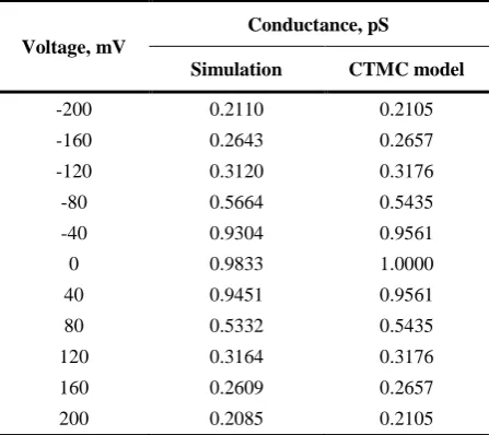
nl .Results are presented in Table 1, which shows
calculated conductances at different Vj values.
Modeling results are obtained from CTMC model and simulation of the GJ channel [4].
Table 1. Voltage-dependent conductance in the GJ channel containing 4 connexins: comparison of simulation and CTMC modeling results
Voltage, mV
Conductance, pS
Simulation CTMC model
-200 0.2110 0.2105
-160 0.2643 0.2657
-120 0.3120 0.3176
-80 0.5664 0.5435
-40 0.9304 0.9561
0 0.9833 1.0000
40 0.9451 0.9561
80 0.5332 0.5435
120 0.3164 0.3176
160 0.2609 0.2657
200 0.2085 0.2105
Table 1 shows that CTMC model and simulation produce similar results. Calculation was performed using a PC with Intel Core 2 Duo CPU T9400 @
2.53 GHz 2.53 GHz and 4 GB of physical RAM.
Preliminary data showed [6] that continuous time Markov chain modeling required significantly less CPU time than simulation.
4. Conclusion
Our results shows that the CMCT model of GJ channel is less complex than an analogous DTMC model, so it is possible to apply Markov model creation tools using a/the PLA method. Creation of
infinitesimal generator is derived from the description of system behavior.
In this paper, we showed that the use of CTMC (instead of DTMC) to model GJ channels enables to reduce computation time ~30 times. This can be achieved since the infinitesimal generator of CTMC arising from GJ channel model, is sparse. This ensures
faster creation of infinitesimal generator Q of CTMC
model than the transition matrix P of analogous
DTMC model of GJ channel. Sparsity of Q also
allows using efficient numerical methods to calculate steady-state probabilities.
Acknowledgments
This work was supported by the Research Council of Lithuania for collaboration Lithuania and USA scientists under grant MIT-074/2012.
References
[1] F. F. Bukauskas, V. K. Verselis. Gap junction channel gating. Biochimica et Biophysica Acta-Biomembranes, 2004, Vol. 1662, No. 1-2, 42-60. [2] J. F. Ek-Vitorin, T. J. King, N. S. Heyman, P. D.
Lampe, J. M. Burt. Selectivity of connexin 43 channels is regulated through protein kinase C-dependent phosphorylation. Circulation Research, 2006, Vol. 98, No. 12, 1498-1505.
[3] K. Bang, J. Choi, C. Yoo. Comments on "The Model Checker SPIN". IEEE Transactions on Software Engineering, 2001, Vol. 27, No. 6, 573-576.
[4] N. Paulauskas, H. Pranevicius, J. Mockus, F. F. Bukauskas. Stochastic 16-State Model of Voltage Gating of Gap-Junction Channels Enclosing Fast and Slow Gates. Biophysical Journal, 2012, Vol. 102, No. 11, 2471-2480.
[5] N. Paulauskas, M. Pranevicius, H. Pranevicius, F. F. Bukauskas. A Stochastic Four-State Model of Contingent Gating of Gap Junction Channels Containing Two "Fast" Gates Sensitive to Transjunctional Voltage. Biophysical Journal, 2009, Vol. 96, No. 10, 3936-3948.
[6] H. Pranevicius, F. F. Bukauskas, O. Pranevicius, M. Pranevicius, S. Vaiceliunas. Markov models of voltage gating of gap junction channels. Invited presentation at 25th Conference on Operational Research (EURO-2012), Vilnius, Lithuania, 2012. [7] H. Pranevicius, V. Germanavicius, G. Tumelis.
specified by PLA method. In: 12th International Conference on Analytical and Stochastic Modelling Techniques and Applications (ASTMA 2005), Nottingham, United Kingdom, 2005, pp. 118-124. [8] H. Pranevicius, R. Miseviciene. Verification of
business rules using logic programming means. In: Modelling of Business, Industrial and Transport Systems, Riga, Latvia, 2008, pp. 99-106.
[9] H. Pranevicius, S. Norgela. Applications of Finite Linear Temporal Logic to Piecewise Linear Aggregates. Informatica, 2012, Vol. 23, No. 3, 427-441.
[10] H. Pranevicius, V. Pilkauskas, G. Guginis. Creating simulation models specified by PLA using UML. In: International Conference on Operational Research: Simulation and Optimisation in Business and Industry, Kaunas, Lithuania, 2006, pp. 87-92.
[11] H. Pranevicius, L. Simaitis, M. Pranevicius, O. Pranevicius. Piece-Linear Aggregates for Formal Specification and Simulation of Hybrid Systems:
Pharmacokinetics Patient-Controlled Analgesia. Elektronika ir Elektrotechnika, 2011, No. 4, 81-84. [12] H. Pranevicius, E. Valakevicius, M. Snipas.
Complexity of embedded chain algorithm for computing steady state probabilities of Markov chain. Information Technology and Control, 2011, Vol. 40, No. 2, 110-117.
[13] A. Sakalauskaite, H. Pranevicius, M. Pranevicius, F. Bukauskas. Markovian Model of the Voltage Gating of Connexin-based Gap Junction Channels. Elektronika ir Elektrotechnika, 2011, No. 5, 103-106. [14] G. Sohl, K. Willecke. Gap junctions and the connexin
protein family. Cardiovascular Research, 2004, Vol. 62, No. 2, 228-232.
[15] G. E. Sosinsky, B. J. Nicholson. Structural organization of gap junction channels. Biochimica et Biophysica Acta-Biomembranes, 2005, Vol. 1711, No. 2, 99-125.