TWO-DIMENSIONAL VECTOR QUANTIZER WITH VARIABLE
LENGTH LOSSLESS CODE FOR LAPLACIAN SOURCE
Milan R. Dincic, Zoran H. Peric
Faculty of Electronic Engineering, University of NisAleksandra Medvedeva 14, 18000 Nis, Serbia e-mail: [email protected], [email protected]
Abstract. The main aim of this paper is to apply variable length lossless code on output points of the sional vector quantizer for Laplacian source. This problem is not yet solved in the literature. In this paper two-dimen-sional quantizer is designed using Helmert transform and its optimization is done. New lossless code is introduced. It is very simple but very close to the ideal code since it gives the bit-rate very close to the entropy. It is applied on the two-dimensional quantizer. It is shown that our two-two-dimensional quantizer can achieve the same performances as scalar uniform and nonuniform quantizers, but using much smaller number of points per dimension. Therefore, two-dimen-sional quantizer has smaller execution complexity.
Keywords: vectorquantizer, lossless code, Golomb-Rice code, execution complexity.
1. Introduction
Quantization is very important step in the process of analog to digital conversion. Quantization is used in almost all modern telecommunication systems. Good choice of quantizer can increase signal quality and decrease bit-rate.
Quantizers can be scalar and vector. Design of some types of scalar quantizers were analyzed in [1, 2, 3]. Vector quantizers give better performances (higher signal-to-quantization noise ratio (SQNR) for the same bit-rate) compared to scalar quantizers, since they have a higher degree of freedom for choosing the re-construction values and the decision regions [4]. But, vector quantizers are, in general case, more complex than scalar quantizers, and their complexity increases with increase of quantizer dimension [4]. Two-dimen-sional quantizers are the simplest, and therefore the most often used vector quantizers.
Lossless compression codes can be used for coding of symbols of discrete sources, decreasing bit-rate. Representation points of quantizer can be considered as symbols of discrete source, and therefore they can be coded with lossless codes. Huffman code is the most popular lossless code [5, 6, 7, 8, 9]. But, the complexity of Huffman code drastically increases when the number of symbols increases, since it is needed to form code tree in coder, as well as in de-coder. Also, probability for each symbol has to be calculated. Because of that, Huffman code is inap-plicable for sources with large number of symbols. Huffman code can be used for coding of levels of
scalar quantizer, if the number of levels is not too large (for example, few tens). But, the number of points of two-dimensional quantizers can be very large. Because of that, Huffman code is practically inapplicable for scalar quantizers with large number of levels and for two-dimensional quantizers.
A simple lossless code was proposed in [10] and it was applied on scalar, but not on vector quantizers. Another important lossless code is Golomb-Rice code. It is much simpler for realization than Huffman code, since this code is computed with a few logical operations and there is no need to form code tree [11, 12, 13]. This feature is especially important for the decoder, which has to be simple and fast. It was proved that Golomb-Rice code is especially suitable for Laplacian source. Due to all these facts, Golomb-Rice code is included in many modern compression standards, such as JPEG-LS [14], MPEG-4 ALS (Au-dio Lossless Coding) [15], and CCSDS (Consultative Committee for Space Data Systems) recommendation for lossless data compression [16]. Also, Golomb-Rice code can be used for compression of test data [17]. Golomb-Rice code was applied on scalar quantizer in [18, 19]. But, application of Golomb-Rice code on vector quantizers has not been analized by now, as we know. So, we can conclude that application of lossless code on vector quantizer is an open problem, not yet solved in the literature. In this paper we propose a solution for this problem.
dimensional quantizer. Firstly, design of two-dimen-sional quantizer is done for memoryless Laplacian source, using Helmert transform [20]. The quantizer is designed in the way that one coordinate (denoted with r) is quantized using hybrid quantizer (combination of uniform and nonuniform quantizers) and the other coordinate (denoted with u) is quantized using uni-form quantizer. It is proved in this paper that hybrid quantizer is the best solution for r coordinate, better than uniform and nonuniform quantizers. The comp-lexity of the hybrid quantizer is between complexities of the uniform and the nonuniform quantizers. Quan-tizer’s cells are placed in concentric rectangular rings. Optimization of the number of cells in each ring is done. After that, a new lossless code is defined. This lossless code is a modification of Golomb-Rice code, but it is more flexible than Golomb-Rice code. Our code gives the bit-rate which is very close to the entropy of the source. The main advantage of our lossless code is its simplicity. It is drastically simpler than Huffman code since there is no need to form a code tree and also there is no need to calculate probabilities of representation points. Therefore, the lossless code can be very easily applied on two-di-mensional quantizers with large number of points. It is shown in the paper that two-dimensional quantizer with variable length codewords can achieve much better performances, compared to scalar uniform and nonuniform quantizers, using the same number of points per dimension (or, in other words, our model can achieve the same performances using much smaller number of points per dimension). For example, our model can satisfy the G.712 standard using in average 92 points per dimension, which is much smaller compared to 128 points needed for scalar nonuniform quantizer or 256 points needed for scalar uniform quantizer. Therefore, our model has smaller execution complexity, and it is faster.
This paper is organized as follows. In Section 2, design of two-dimensional quantizer is described using Helmert transform, expressions for distortion are derived, optimal numbers of cells in rings are calculated and the lossless code is described. Section 3 gives some numerical results. In Section 4, some addi-tional explanations are given and execution comp-lexity of our model is discussed. Section 5 concludes the paper.
2. Design of the two-dimensional quantizer with the lossless code
2.1. Helmert transform
The 2-D (two-dimensional) probability density function for independent identically distributed La-place random variables (source) with zero mean and the unity variance is given as
1 2 2 2 1 )
( e x x
f x , (1)
where is the source vector with elements and . To simplify the vector quantizer, the Helmert transform [20] is applied on the source vector. This transform is defined as mapping
, so that x
) ,S
1 x
2 x
,
(x1 x2 (r,u,A)
1 2
2 1
x x
r ;
1 2
2 1
x x
u ;AS, (2)
t
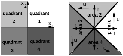
where S represents the quadrant where the point is placed. S can take values from the set . These quadrants are presented in Figure 1(left). A represents the area where the point is placed, and A also can take values from the set
. These areas are presented in Figure 1(right). Point ) from the quadrant i is map-ped into poin ,u) in the area i, . These additional information S and A about quadrants in
domain and about areas in domain are needed to provide one-to-one mapping, i.e. to provide uniquely defined transform. Based on the expression (2) and Figure 1b, we can conclude that
) , (x1 x2
} 4 , 3 , 2 , 1 {
} 4 , 3 , 2 , 1 {
) , (x1 x2
) , (r u
4 ,
(x1 x2 (r
i1,2,3,
) , (r u
r 0
and rur,r.
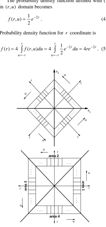
Effect of Helmert transform is rotation of the coor-dinate system for 45 degrees clockwise, i.e. coordinate system is obtained by rotation of (
coordinate system for 45 degrees clockwise. This is shown in Figure 2.
) , (r u
) , 2 1 x x
quadrant
4 quadrant
2
quadrant
3
quadrant
1 x 1 x2
ar
e
a
1
area 2
are
a 3
area 4 r r
r
r
u u
u
u
Figure 1. Quadrants in the domain (left) and areas in the domain (right)
) , (x1 x2 ) u , (r
Inverse mapping (r,u,A)(x1,x2,S) is defined as:
r u
x
2 1
1 ; x
ru
2 1
2 ;S A. (3)
Based on S and using (3), and are calculated in the following way:
1
x x2
1 x 1
x if S{1,4};
1
1 x
x if S{2,3}; x2 x2 if S{1,2};
2
2 x
The probability density function defined with (1), in (r,u) domain becomes
r e u r
f 2
2 1 ) ,
( . (4)
Probability density function for r coordinate is
r r
r u
r r
r u
re du e du
u r f r
f 2 4 2
2 1 4 ) , ( 4 )
(
. (5). . . . . .
. . .
. . .
. . .
. . .
u
u u
r r
r
x2
x1 r u
. . .
. . .
. . .
. .
.
. .
.
. . .
. . .
. . .
. . .
area 4
ar
ea
3
area 2
u u
u
r r
r
r u
ar
ea
1
. . .
Figure 2. Due to Helmert transform, coordinate system is obtained by rotation of coordinate
system for 45 degrees clockwise
) , (r u
) , 2 1 x (x
2.2. Two-dimensional (2D) quantizer
Now, we will define two-dimensional quantizer in domain. The total number of cells of that quan-tizer is N. For
) , (r u
r coordinate, hybrid quantizer will be applied. For u coordinate, uniform quantizer will be applied.
Quantization of rcoordinate. As it was said, hybrid quantizer is used for quantization of r
coordinate. This hybrid quantizer is combination of a uniform and a nonuniform companding quantizers. r*
denotes the value of r coordinate which is the border between uniform and nonuniform quantizers. Uniform quantizer consists of L1 levels for r coordinate. Thre-sholds for this uniform quantizer are denoted by
1 ,..., 0
,i L
ri and they can be calculated as
. It is valid that and .
Representation levels for uniform quantizers are . Nonuniform quanti-zer for
1 *
/L ir ri
) 2 / 1 (i
mi
0 0
r *
1 r rL
1 1
*/L ,i 1,...,L
r
r coordinate is companding quantizer with
optimal compression function ,
which is defined as [1]:
) 1 , 0 (
)
, * r ( : ) (r g
* *
) (
r r
r r g
) (r f
) (r g
3 3
) (
) (
dr r f
dr r f
. (6)
For defined with (5), compression function becomes
3
2 , 3 2 E 3
3 2 , 3 1 E
1 *
* *
r
r r
2*/3
e r
2 ) (r
g
3 2 , 3 2 E 3 2 /3
3 / 1
*
r e
r
r r
, ( E a
2
L
, (7)
where is exponential integral
function, which is very suitable for numerical computation. Nonuniform companding quantizer has
levels. Thresholds for this nonuniform quantizer are denoted by
1
) e t dt
z zt n
* L r
r 1 rL11...rL1L21
2
1 L
L r
1 1 1 L
L m
m
. Representation levels are denoted by
2 1
... 2 mLL
. Thresholds and
represen-tation levels for nonuniform quantizer can be found by numerical solving of the following equations:
2 1
) (r i g i
L L
,iL11,...,L1L2 1, (8)
2 1 1
1 2
,..., 1 ,
2 1 1
) (m
g i i L i L L L
L
.(9)
There are totally L1L2 levels for r coordinate.
Each level for r coordinate makes one ring in two-dimensional plane. Therefore, we have totally L1L2
concentric rings. The area which consists of the first rings (where
1
L r coordinate is uniformly quantized) is called uniform part of 2D quantizer, and the area which consists of L2 rings where r coordinate is non-uniformly quantized is called nonuniform part of 2D quantizer.
Quantization of coordinate. Inside each ring, uniform quantization of ucoordinate is done. On the i-th ring we have levels for u coordinate, in each of four areas. Thresholds for u coordinate on
u
i
the i-th ring ( ) are denoted by and representation levels are
denoted by . For rings
2 1
,...,
1 L L
i
i
i
M j1,...,
j
i j M
u, , 0,..., , ˆi,j
u i1,...,L1L21, quantization cells Si,j
ri1,ri
;
ui,j1,ui,j
1
are rect-angular, which is shown in Figure 3 (up). The quan-tization stepsize for u coordinate on the i-th ring,
, is ,...,
1 1 2
L L
i
i i i
i i i
M r r
4 /
1
1
L
i
u
M r (
4 1
2
L
r)
. (10)
On the ( )-th ring, quantization cells
L2,j
2 1 L
L
L j 1 u
, 1
2 ,
u L L
u 1 ;
,
L L1 21
j L
L r
S 1 2, are also
rectangular, but unbounded on the one side. This is shown in Figure 3 (down). For the ( )-th ring, the quantization stepsize for coordinate is
2 1
2 1 2
1 2 1 1
4 /
L L L
j i S,
1 N
N
D
3 D1
2 1 L
L
3 D
2 1 L
L
u
, (mi
2 1
11
2
L L
L i
N
2
N
1 D
D
D
1
2 1L L
D D1 D
1
8
L L
L L
M r
2
L
M r
) ˆi,j u
N
4
i
M
2D
3 D
2
1 D
. (11)
Within each cell there is one representation point . There are four overload cells which are presented in Figure 3 (down). Within each of these four overload cells there is one representation point, which will be defined later. The total number of quantization cells of two-dimensional quantizer is
denoted with . is the total
number of cells in the uniform part, and
is the total number of cells in the
nonuniform part. Additional four cells in the expres-sion for are overload cells.
2
1
L
i
N 1
1
i
M
2 D 2.3. Distortion
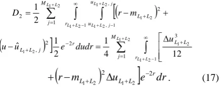
The total distortion consists of three parts, i.e., . is distortion in the first rings where cells are bounded; is distortion in the ( )-th ring, where cells are unbounded; is distortion in four overload cells. This is shown in Figure 4. All these distortions ( , , and ) are distortions per dimension. Usually, for vector quantization, distortion is given per dimension, to simplify comparison of performances of vector quantizers with different dimensions.
Distortion is given with the following expression:
2
1
1 2
1
i m r
D
1 1 1
, ,
M
j r
r u
u i i
i j i
j i
2 1
1 L
L
i
j 2 e2rdudr
2 1
u
uˆi, . (12)
. . . . . .
r
i
-1+
r
i
r
i
u
r
. .
.
. . .
. . .
. . .
. . .
u u
u
r
r
r . . .
r
i -1
ui
cells cells
cells .
. .
. . .
mL1+L2 r
r r
r rL1+L2-1
unbounded unbounded
unbounded unbounded
. . .
. . . cells
overload overload overload
overload cell cell
cell
cell
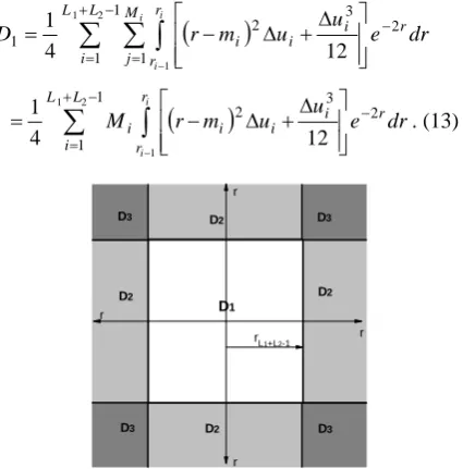
Figure 3.Rectangular cells on the i-th ring, i1,..., 1
2
1L
L (up); unbounded rectangular cells and four overload cells on the (L1L2)-th ring (down) The factor 1/2 at the beginning of the expression (12) means that is distortion per dimension. After integration by uit is obtained:
1
D
1
1 1
2 3 2
1
2 1
1 12
4 1L L
i M
j r
r
r i i i
i i
i
dr e u u m r D
1
1
2 3 2
2 1
1 12
4 1L L
i
r
r
r i i i i
i
i
dr e u u m r
M . (13)
r
r r
r rL1+L2-1
D1
D2
D2
D2
D2
D3
D3
D3
D3
Figure 4. Regions where distortions , and are defined
1
For ui defined with (10), we obtain:
1 1 2 1 1 2 1 1 ) ( L L i r r i i i i i m r r r D
e dr M r r r i i i 2 2 2 1 3 ) (4
. (14)
Finally, after basic integration, the following expres-sion is obtained:
2 2 1 2 1 1 1 1 2 2 1 2 1 1 ) ( 3 2 ) 1 )( ( 2 1 4 1 ) ( 3 2 ) ( 2 1 1 i i i r i i i i L L i i i i r i i M r r e m r m r M r r e r r D i i
1 2( )(1 )
4 1
i i i
i m r m
r
. (15)Previous expression (15) can be written as
, where (*)
denotes the expression under summation in (15). denotes distortion in the uniform part (i.e. in the first
rings) and using expressions for and which were defined in Subsection 2. 2., it is obtained that
11 12 1 1 1 1 1 1 2 1 1 1 2 1 * ** D D
D L L L i L i L L i
1L ri
11 D i m
2 1 * 1 * 2 2 2 1 * 1 2 1 * 1 * ) 1 ( 2 1 * 11 2 1 1 4 1 ) / ) 1 2 (( 3 2 2 1 1 4 1 ) 1 2 ( 1 * 1 1 * L r L r e M L r i L r L r e L r i D L r i i L i L r i 2 2 1 * ) / ) 1 2 (( 3 2 i M L r i. (16)
12
D represents distortion in rings L11,...,
; and defined with (8) and (9) should be used in calculation of .
1
1
L L2 ri mi
12 D
Distortion in the ( )-th ring where cells are unbounded, denoted as , is defined as:
2 1 L L 2 D
2 1 1 2 1 2 1 2 1 2 1 1 2 1 , 2 1 1 , 2 1 2 1 1 3 2 2 , 1 2 2 12 4 1 2 1 ˆ 2 1 L L L L L L L L j L L j L L M j r L L r j L L M j r u u L L u dudr e u u m r D . (17)
r mL L
uL L
e rdr2 2 2 1 2 1
After integration and summation, and using (11), it is obtained:
2
2 1 2 1 2 2 1 2 1 1 2 1 2 1 3 16 L L L L r L L M r e r
D L L
2( )(1 ))
1 ( 2 1 2 1 2 1 2 1 2
1 L 1 L L L L 1 L L
L m r m
r .(18)
The overload distortion represents distortion in four overload cells. In each overload cell there is one representation point. To minimize distortion, this representation point should be placed on the bisector of the overload cell. Therefore, values of r and u coordinates of the representation point are equal and denoted with c. The overload distortion can be
calculated as , where
3 D half 3 D 3 D 3 8
D D3half
21
1 1 21
2 2 2 1 2 1 L
L L L
r r r u r e c u 2 c
r dudr
repre-sents distortion in the half of the one overload cell. This is shown in Figure 5.
(c,c)
Dhalf3
representation point
Figure 5. One overload cell with the representation point placed on the bisector of the overload cell After integration, it is obtained that
1 2 1 2
3 1 2 1 2
1 2 1 2 4 7 L L L L r r r e
D L L
1
. (19)2
2 1 2
2
c c crL L
Minimizing D3, 2 2 2 1 0
3 2 1 L L r c c D , we
obtain the optimal value for parameter c
1
2 1 1
rL L
c . (20)
Changing this into (20), we obtain the following expression for the overload distortion
1 2 1 2 3 4
3
rL L
e
D . (21)
The total distortion D is equal to the sum of expressions (15), (18) and (21). Signal-to-quantization noise ratio (SQNR), for unit variance, is defined as:
D
2.4. Optimal number of cells on rings
In this subsection, optimal values of the number of cells on each ring, denoted with Mi,i1,...,L1L2
1 1 1 N M L i i
, will be found, in the way to minimize distortion D.Two condition must be fulfilled: and
. So, minimization of D with these
constraints should be done, and this will be done using the technique of Lagrange multipliers. Firstly, we define function J in the following way:
4 2 1 2 1 1
N M L L L i i , ) 4 ( 2 1 1 1 1 2 2 1 1 1
L L L i i L i i N M N M D J (23)where 1 and 2 are Lagrange multipliers. Now,
minimization of J will be done. For Mi,i1,...,L1 it is valid that
. 0 ) 1 2 ( 3 4 1 2 ) 1 ( 2 3 1 * 3 1 11 1 1 * 1 * L r i L r i i i i i e e L r i M M D M D M J (24)
From (24) it follows that
3 2 3 2 1 * 3 1 1 3 4 ) 1 2 ( 1 1 * 1 *
L
r
L r i
i e e
L r i M , . (25)
Changing these values in the condition ,
it is obtained that
1 ,..., 1 L i
1 1 1 L j j N M
1 1 * 1 * 1 3 2 3 2 1 * 1 3 1 ) 1 2 ( 1 3 4 1 L j L r j L r e j e L r N . (26)Changing this in expression (25), we obtain expressions for the optimal values of the numbers of cells in rings in the uniform part:
1 1 * 1 * 1 3 2 3 2 1 ) 1 2 ( ) 1 2 ( L j L r j L r i i e j e i NM ,i1,...,L1. (27)
For Mi,iL11,...,L1L21 it is valid that
2 12 2 i i i M D M D M J
03 4 2 2 2 3 1 3
1
ri ri
i i i e e r r
M . (28)
From the previous expression it follows that
3
2 2
1 3 2 1 3 4 1 i i r r i i
i r r e e
M
,
iL11,...,L1L21. (29)
For ML1L2 it is valid that
. 0 3 32 2 2 3 1 3 2 2 2 1 2 1 2 1 2 1 2 1 2 1 2 1 L L r L L L L L L L L L L e r M M D M D M J (30)
It follows that
3 2 1 3 2 1 2 1 2 1 2 1 3 4
2
L L L rL L
L r e
M
. (31)
Changing expressions (29) and (31) into condition
, it is obtained that
2 1 1 1 2 4 L L L j j N M 1 3 2
2 3 2 1 2 1 2 1 3 4 2 4
1 rL L
L L e r N
1 13 2 2
1 2 1 1 1 3 4 L L L j r r j j j j e e r
r . (32)
Changing this into (29) and (31), we obtain optimal values of cells number for rings in the nonuniform part: , 2 ) ( ) )( 4 ( 3 2 1
3 2 2
1 1
1
3 2 2
1 2 1 2 1 2 1 1 2 1 1 1
j j L Li i r L L r r L L L j j j r r i i i e r e e r r e e r r N M 1 ,...,
1 1 2
1
L L L
i , (33)
1
3 2
1
2 1 2
1 2 1 2 1 2
1 ( 4)2 2L L
r L
L L
L N r e r
M L L
1
1
3 2 2
1
3 2 1 2
1 1 1 2 1 L L L j r r j j
rL L j j
e e r r
e . (34)
2.5. Regions making and modification of the number of cells
first L1 rings), we make S L1/k regio c
ns, by joining
k conse utive rings in one region. It is valid that the
i
-th region (i1,.. nsists of rings . The whole nonuniform part (with rings and cells) is one, the (S
., ) co
ik
2 N k i 1) ( ,
1
2 L k ) 1 i
( 2,...,
1 S
1
)-th region. Four overload cells also belong to )-the (S1)-th region. Therefore, we have totally S
k j M
1
regions. , denotes the number of cells
in the -th region. It is valid that for
, where are given with (27). Also, it is valid that .
i
Q i1
S
1 QS
1 ,...,S
j M
2 N i
,..., 1
ik
i j i Q
) 1 (
i
To apply the lossless code, one condition should be fulfilled: the number of cells within each region must be a power of two, i.e. Q 2 i, i1,...,S1;
i
i
. Firstly, we will consider regions in the uniform part. For given with (27), this condition is not satisfied in general case. Therefore, we should modify the number of cells in regions in the uniform part. With ] is denoted the nearest number of which is the power of two. [x] is the nearest integer of the real number x. Now, instead of
cells, each region in the uniform part has Qi* ce
Since the number of cells in regions is modified, the number of cells in rings also should be modified. The modified number of cells in the j-th ring, which is in
the i-th region, is ,
; . So, inside the -th
region, the total number of cells is changed by
*
cells, and this change is equally distributed on all rings inside this region, i.e., the number of cells in each ring in this region is changed by
. It is valid that . The
modified number of cells within the uniform part is
. So, on the beginning of the design
process the cells number in the uniform part was set to the initial value . This initial value is chosen to achieve required performances (for example, if the G.712 standard should be satisfied, SNR higher that 34 dB should be achieved). But during the design process this initial value is modified, and we obtain new number of cells in the uniform part, denoted with
*
. * is usually very close to the initial value .
j
M
[log2
2
k i1)
1
N
* Qi
i Q
i Q
j( 1,...,
i Q
i1,...,
i
i Q
Q
k
Q Qi i
( *
1
1 * 1
L
i
N
1
N N1
lls.
k Q Q
Mj i i
j ( )/
*
*
ik i
ik
k i j
j
i M
Q
1 ) 1 (
* *
1
N
1
N M
S
/ )
M k
*
i
Since the whole nonuniform part is one region, the number of cells in the nonuniform part must be a power of two. If the initial number of cells is not a power of two, it should be changed with *
, the
nearest integer to which is a power of two. So, . Then, modified numbers of cells in rings
in the nonuniform part are ,
2 N
N2
2 N
2 L
* 2 *
1 N
QS
1 1,..., L j
2 * 2 2 *
/ )
(N N L
M
Mj j
1 L
.
Now, modified values M*j, j1,...,L1L2
1
i
should be used in expressions (15) and (18), instead of initial values Mi.
2.6. Lossless code with the variable length codewords
In this section the lossless code will be described. As it was said, we have regions. Within the i-th region there are representation points (one point in each cell). One index
S
*
i Q
( ) can be
assigned to each point in the i-th region. Points are coded with codewords using the following coding rule:
1 0i Qi*
1 1
Rule 1). Point from the i-th region, ( iS ) with index i is coded with codeword ,
where is the natural binary code of the index
* 2
log 1
... 0 1 ... 1
i
Q i
x x
2
log
... x
i
*
i
Q
x
. All points within one region are coded with codewords with the same lengths li ilog2Qi*.
i
This lossless code is a modification of Golomb-Rice code. In Golomb-Golomb-Rice code [8] numbers of cells in each region should be the same, i.e.
* *
. In our code, numbers of cells in different regions can be mutually different. Therefore, our code is more flexible than Golomb-Rice code and there are more possibilities to obtain required per-formances by adjusting the number of cells in regions.
1
S
2 * 1 Q
Q ...Q
Now, we will explain how to assign index to points in some region. Let’s consider the i-th (1iS) region in the uniform part. In this region there are k rings: (i1)k1,...,ik. Index assignment procedure is defined with the following three rules:
Rule 2). Rings are coded in increasing order, i.e. ring (i1)k1 is coded firstly, after that ring
2 ) 1 (i k
(
M
2 ) 1 (i k
M
1 *
2 ) 1 (i k M
2 ) 1 (
,…, and finally ring ik. This means that
the first * indexes ( ) are
assigned to the points in the ring ; the next
*
indexes (
) are assigned to the points in the ring
1 ) 1
k
i 0 1
* 1 ) 1
(
i M i k
1 ) 1 (i k
(* 1) 1
* 1 ) 1
(i k i M i k
M
k
i
1
*
i
i Q
;…; the last indexes (
) are assigned to the points in the ring
*
ik
1
1 *
) 1 (
k
j
j k i
M
Rule 3). Within each ring, points from Area 1 are coded firstly, after that points from Area 2, after that points from Area 3 and finally from Area 4. For example, in the ring (i1)k1, indexes 0i
i
2 /
are assigned to the points in Area 1,
indexes to the
points in Area 2, indexes
to the points in Area 3 and indexes
to the points in Area 4. Using this rule, information about the area where some point belongs is included in index (and therefore in the codeword) and there is no need to transmit additional information about the area. Based on the received codeword, receiver can determine to which area this point belongs. Recall that the receiver must know information about the area for calculation of the inverse Helmert transform (see Subsection 2.1.).
1 4 /
* 1 ) 1 (i k
M
k
i M(* 1)
1 4 / 3M(*i1)k1
k
i
M /4
3 (*1) 1
i *
) 1 (i M
1 *
1 ) 1 (i k
1/4
i 3M
1 2 /
1
k
k i
M(* 1) 1
Rules 2) and 3) can be joined in the following rule:
Rule 2-3). Indexes which are assigned to the points in the i-th region, in the ring, in the
m-th area ( ; ; 4 ) should
satisfy the following condition:
p k i1) (
k m1,2,3 S
i1,..., p1,..., ,
. ,..., 2 for , 1 4 /
4 / )
1 (
; 1 for , 1 4 /
4 / )
1 (
* ) 1 ( 1
1 *
) 1 (
* ) 1 ( 1
1 *
) 1 (
* 1 ) 1 (
* 1 ) 1 (
k p mM
M
M m M
p mM
M m
p k i p
j
j k i
i p k i p
j
j k i
k i
i k i
(35)
Rule 4). Within each area in some ring, order of the points is defined with increase of the u coordinate. This means that within each area in some ring, the smallest index is assigned to the point with the smal-lest u coordinate and the highest index is assigned to the point with the highest u coordinate.
Now we will consider assignment of index i in
the nonuniform part. Index i can take values
. In the nonuniform region, rules 1), 3) and 4) are the same as for the uniform part. Rule 2) should be slightly modified, and it will be denoted as Rule 2’).
1 0i N2*
Rule 2’). Rings are coded in increasing order, i.e. ring L11 is coded firstly, after that ring L12,…,
and finally ring . The highest four indexes
( ) are assigned to
the four overload representation points.
2 1 L
L
, 3
*
2 N ,
4 N2* i
*
2
N 2,N*21
For the nonuniform part, rules 2’) and 3) also can be joined in one rule:
Rule 2’-3). Indexes which are assigned to the points in the -th region, in the ring, in
the m-th area (
) 1
(S L1 p
2
,...,
1 L
p ; ) should satisfy
the following condition:
4 , 3 , 2 , 1
m
,..., 2 for , 4
; 1
p p
i i
) 1
S M*i (i
i
. (
(
2 1
1 * 1
1 *
*
1 1
L M
M mM
m
p
j j L p
j j L
L
1 4 /
/ ) 1
for , 1 4 /
4 / ) 1
* * 1
* 1
1 1 1
1
mM M m
M
p L
p L L
,..., 1 (
* i
Qi
i
(36)
Decoding process in the receiver. There is a decoder for lossless code in receiver. This decoder re-ceives codewords, and it should decide which repre-sentation points were coded with these codewords. The decoder has to know the following
parame-ters: , , k, , .
This requires some memory space, but this memory space is very small (1kbit is enough in the most cases, which is not a problem in today electronic systems). Since , we can store
1 L
Q 2 L
i
*
) ,..., 1 L1L2
2 instead of , to
save the memory space. Decoder uses Rules 1), 2-3), 2’-3) and 4) in the decoding process.
*
i Q
Decoding process is very simple. Decoder receives bit-stream and it should start with decoding process, i.e. it should decode the first codeword. Suppose that decoder knows which bit is the beginning of the first codeword. But, decoder does not know the length of the codeword (since it is variable). Decoder starts decoding of the codeword by counting consecutive 1’s on the beginning of the codeword, until the first 0. This number of consecutive 1’s is denoted with z, and decoder knows (using Rule 1) that . It follows that the region i where the point belongs is
1 i z
1 z
i .
Knowing i, decoder reads from its memory parameter and calculates the length of the codeword as
. Now, decoder knows where the end of the codeword is and where the next codeword begins. The last bits of the codeword is the natural binary code of the index
*
i Q
i
l i*
* 2 log Qi 2
log Q
i
i
, and converting this natural binary code into integer, the index i is
obtained. Knowing the index i and reading
parameters from its memory,
decoder can apply Rule 2-3) if or Rule 2’-3) if
) 2 L
S i 1 ,..., 1
( 1
*
L i
i
M
1
S
2.7. Bit-rate
The bit rate R is defined as
1
1 2 1S
i i iP l
R [bits/sample]. (37)
The factor ½ means that R is bit-rate per
dimension. is the length of the
codewords in the i-th region. is the probability of the i-th region, and it is defined with the following expression
* 2
log i
i i Q
l
i P
* *
*
. 1 ,
) , ( 4
; 1 , ) , ( 4
/
/ ) 1 (
r r
r
r u
S ir
S r i r
r
r u i
S i dudr u r f
S i dudr u r f
P (38)
For defined with (4), expression (38) be-comes
) , (r u f
. 1 ,
2 1
; 1 , / 2 1
/ ) 1 ( 2 1
* 2
* /
2
* /
) 1 ( 2
* * *
S i r e
S i S ir e
S r i e
P
r
S ir S r i
i (39)
3. Numerical results
In this section some numerical results for our two-dimensional quantizer will be given. We will present two examples.
Example 1. Let’s consider two-dimensional quantizer with parameters: N1 9216, ,
11 2 2
N L164,
, . The optimal value for
16 2
L k8 r* is chosen
to optimize performances. For this example, the optimal value is . Using expressions (22) and
(37), it is obtained that and
bits/sample. Entropy is
5 . 4 * r
dB 04276 . 6 2462 . 34 SNR 08946
. 6
R H
i p
2 N
2
N
bits/sample (entropy is calculated using well-known
expression where represents
point’s probability, and summation is done over all points). This quantizer is designed to satisfy the G.712 standard. The modified number of points in the uniform part is . Since is a power of two, there is no need to modify the number of points in the nonuniform part, i.e. .
i
p log2(1/pi)
8444 * 1
* 2
N i
N
Simulation in MATLAB for this example is done for memoryless Laplacian source. Results of the simulation are: SNR34.2447dB and R6.0435
bits/sample. We can see that simulation and theoretical results are very close (almost identical). In that way,
correctness of the theory developed in Section 2 is proven.
The average number of points which is used during
the quantizer’s work is 1 2*
* 1 1)
1
( P N P N
N S S
(explanation – cells in the uniform and in the nonuniform part are not used simultaneously; instead of that, in one moment only cells in the nonuniform part are used with probability given with (39), or only cells in the uniform part are used with the probability
1 S P
1
1PS ). For the aim of comparison with scalar quantizers, we can define equivalent scalar quantizer of our vector quantizer, whose the average number of points used during quantizer’s work is
N
Nav (measured in points per dimension).
shows the execution complexity (complexity of execution of coding and decoding algorithm), which is very important for the speed of the execution. For this example it is obtain that points. So, our model can satisfy the G.712 standard with 92 points per dimension in average. It is known [1] that scalar uniform quantizer can satisfy the G.712 standard using 256 points and scalar nonuniform quantizer using 128 points during the process of execution. So, we can conclude that our model can satisfy the G.712 standard using much smaller number of points per dimension during the execution process, compared to scalar uniform and nonuniform quantizers. Therefore, the time that is needed for coding and decoding process is shorther.
av
N
92
Nav
Example 2. In this example, we will consider the two-dimensional quantizer with the following parameters:
256 1
N , N2 64, L1 8, L2 4, k2
*
. For these parameters, the optimal value for r is
. It is obtained that ,
8 . 2 *
r
7586 . 3
dB 2187 . 19
SNR
R
, 11 {
bits/sample and H bits/sample. Since this quantizer has small number of rings, the design process will be described in more details. In the uniform part we have 8 rings. Using expression (27), we calculate numbers of points in these rings:
678 . 3
} 32 , 36 , 38 , 39 , 39 , 35 , 26 i
M . Now, we join two
successive rings (k2 } 68 , 77 ,
) into one region with
74 , 37 { i
Q
, 32 { *
i Q
224 * 1
N
points. Now, we modify numbers of points in regions to obtain the power of two:
. The modified numbers of points
in rings are: . The
modified number of points in the uniform part is . In the nonuniform part we have four rings with
} 64 , 64 ,
{ *
i
M
, 16 , 16 , 20 { 64
} 32 , 32 , 32 , 32 , 36 , 28 , 24 ,
} 8 8
i
M points and four overload
points. Since is a power of two, there is no need to modify the number of points in the nonuniform part. Here it is valid that points per dimen-sion. It is known [1] that scalar uniform quantizer with 16 points (i.e. bit-rate of 4 bits/sample) gives
2
N
96 . 15
SNR
256 1
N
dB and scalar nonuniform quantizer with 16 points gives dB. So, our model gives much better performances using smaller number of points per dimension, compared to scalar uniform and nonuniform quantizers.
13 . 18
SNR
1
L
*
From these examples we can also conclude that the lossless code is very efficient, since the bit-rate R is very close to the entropy H, i.e. the lossless code is very close to the ideal code.
4. Discussion
In this section we will give some additional explanations and remarks about our model.
1) Why a hybrid quantizer is used for r coordinate
quantization? As it was said, hybrid quantizer is a combination of uniform and nonuniform quantizers. Both of them have some good characteristics. Uniform quantizer is very suitable to use together with lossless code, giving small bit-rate. Nonuniform quantizer gives higher SNR. Hybrid quantizer joins good charac-teristics of both uniform and nonuniform quantizers. Now, two examples will be given (the first where only uniform quantizer is used for r coordinate and the second where only nonuniform quantizer is used for r coordinate), and comparison with Example 2 (where hybrid quantizer is used for r coordinate) will be done.
Example 3. Two-dimensional quantizer where only uniform quantizer is used for r coordinate, with
points and rings. In this case optimal range of the uniform quantizer is . Since there is no nonuniform quantizer in the outer part, when
8
6 *
r
r
r we have overload distortion. It is
obtained that and
bits/sample. These results can be compared with results of Example 2 (where hybrid quantizer for r coordinate was used) We can see that the bit-rate is almost the same, but SNR is much higher (for 5 dB) when hybrid quantizer for r coordinate is used. Therefore, hybrid quantizer for r coordinate is better than uniform quantizer.
dB 2018 . 14
SNR
dB R
6991 . 3
R
Example 4. Two-dimensional quantizer with 256 points and 16 rings, where only nonuniform quantizer is used for r coordinate. Performances are:
and bits/sample. We
can see (from Example 2) that when hybrid quantizer is used for r coordinate, almost the same SNR is achieved with smaller (for 0.47 bits/sample) bit-rate R. Therefore, hybrid quantizer for r coordinate is better than nonuniform quantizer.
1085 . 19
SNR 4.222
So, we can conclude that hybrid quantizer is the best solution for quantization of r coordinate.
2) Execution complexity. It was shown in Section 3 that our model can achieve the same performances using smaller number of points per dimension, com-pared to scalar uniform and nonuniform quantizers.
This means that our model has low execution complexity. Now, we will further analyze execution complexity of the model, which is equal to the sum of the execution complexity of the two-dimensional quantizer and of the lossless coder.
2a) Execution complexity of the two-dimensional quantizer. It is well known that execution complexity of nonuniform quantizer is much higher than that of the uniform quantizer. As it was said, u coordinate is quantized with uniform quantizer, which is simple. r coordinate is quantized with hybrid quantizer, which is the combination of uniform quantizer (which is simple) and nonuniform quantizer. This nonuniform quantizer has small number of levels (equal to ). Furthermore, this nonuniform quantizer is very rarely used, since it is placed in the outer part of the two-dimensional plane (for high r), which has very small probability. The great majority of input vectors (r, u) belong to the uniform part, and then two-dimensional quantizer can be realized as combination of two uni-form quantizers (one for r and one for u coordinate), which is simple. So, we can conclude that nonuniform quantizer for r coordinate does not increase execution complexity of two-dimensional quantizer significantly.
2
L
To better explain this, the quantizer from Example 1 (from Section 3) will be considered. r coordinate is quantized using uniform quantizer with le-vels and nonuniform quantizer with levels. Probability of the nonuniform part is . Now, we will determine how much levels are needed for the uniform quantizer for u coordinate. When we know the ring and the area where some point belongs, uniform quantization for u coordinate should be done only within this area in this ring. So, if the point belongs to the i-th ring, the number of levels of the uniform quantizer is equal to the optimal number of points in that area, which is equal to M , and it varies from one ring to another. For this example, the maximal value of is 65. Therefore, the uni-form quantizer for u coordinate should have maximum 65 levels, but for the most rings this number is smaller. Finally, we can conclude that: in 99.877 % cases, the two-dimensional quantizer is a combination of two uniform quantizers (one with 64 levels for r coordinate and one with maximum 65 levels for u coordinate); in 0.123 % cases the two-dimensional quantizer is a combination of one nonuniform quantizer with 16 levels (for r coordinate) and one uniform quantizer with maximum 65 levels (for u coordinate). Therefore, the execution complexity of this two-dimensional quantizer is smaller compared to scalar uniform quantizer with 256 levels or scalar nonuniform quantizer with 128 levels, which can achieve the same quality (defined with the G.712 standard).
64 1
L
16
0.0012341
1
4 /
*
i
2
L
S P
4 /
*
i M
the complexity of Huffman code is very high, since code tree should be made during the coding process (in transmitter) as well as during the decoding process (in receiver). Because of that, Huffman code is suitable only for discrete sources with small number of symbols. Huffman code can be used for coding of output levels of scalar quantizer if the number of le-vels is not too high. But, the number of representation points for two-dimensional quantizers can be very large. Huffman code is not suitable to be used in combination with two-dimensional quantizers.
Lossless code described in this paper is very simple and it can be very easily applied for coding points of two-dimensional quantizers. For this code there is no need to make a code tree. Coding and decoding processes are very simple – they include counting of 1’s and conversion of index i into
natural binary code (and reverse). This code is a modification of Golomb-Rice code. It is well known that Golomb-Rice code is much simpler than Huffman code [11].
Huffman code also needs knowledge about prob-abilities of every point. Since we have large number of points in two-dimensional quantizer, calculation of these probabilities is very difficult. Our lossless code does not require knowledge of points’ probabilities. This is another reason why our lossless code is much simpler than Huffman code.
It was shown in Section 3 that our lossless code, although very simple, is very efficient, since it gives the bit-rate R very close to the entropy H.
We proved that both the two-dimensional quantizer and the lossless coder have low execution complexity, therefore the total execution complexity of our model is low.
5. Conclusion
In this paper, one solution was given for the problem which had not been considered in literature: application of the lossless code on output levels of the two-dimensional quantizer. Huffman code is inapplic-able for this problem because it is too complex. De-sign of the two-dimensional quantizer was done using Helmert transform, and optimization of the number of cells on rings was done. New lossless code was introduced and applied on the two-dimensional quan-tizer. It is very simple, but it was shown that it is very close to the ideal code, since the bit-rate is very close to the entropy. Simulation in MATLAB was done and theoretic results were proved. It was shown that our two-dimensional model had smaller execution comp-lexity than scalar uniform and nonuniform quantizers, i.e. it could achieve the same performances using much smaller number of points per dimension and faster.
References
[1] N.S. Jayant, P. Noll. Digital Coding of Waveforms.
Prentice-Hall, 1984.
[2] Z. Peric, J. Nikolic, A. Mosic, S. Panic. A switched-adaptive quantization technique using µ-law quantizers. Information Technology and Control, 39(4), 2010, 317-320.
[3] Z. Peric, J. Nikolic, Z. Eskic, S. Krstic, N. Mar-kovic. Design of novel scalar quantizer model for Gaussian source. Information Technology and Cont-rol, 37(4), 2008, 321-325.
[4] A. Gersho, R.M. Gray. Vector Quantization and Sig-nal Compression. Kluwer Academic Publishers, Masa-chusetts, 1992.
[5] D. Hankerson, G.A. Harris, P.D. Jr. Johnson. Introduction to information theory and data comp-ression. CHAPMAN & HALL/CRC, 2ndedition, 2004. [6] K. Sayood. Introduction to Data Compression.
Else-vier Inc., 3rd edition, 2006.
[7] A.R. Elabdalla, M.Irshid. An efficient bitwise Huff-man coding technique based on source mapping.
Computers and Electrical Engineering, 27, 2001, 265-272.
[8] K. Fredriksson, J. Tarhio. Efficient String Matching in Huffman Compressed Texts. Fundamenta Informa-ticae, 63(1), 2004, 1-16.
[9] A. Zolghadr-E-Asli, S. Alipour. An effective method for still image compression /decompression for trans-mission on PSTN lines based on modifications of Huffman coding. Computers and Electrical Enginee-ring, 30, 2004, 129-145.
[10] Z. Peric, M. Petkovic, M. Dincic. Simple Comp-ression Algorithm for Memoryless Laplacian Source Based on the Optimal Companding Technique. Infor-matica, 20(1), 2009, 99-114.
[11] D. Salomon. Variable-length Codes for Data Comp-ression. Springer, 2007.
[12] R.F. Rice, P.S. Yeh, W.H. Miller. Algorithms for high speed universal noiseless coding module. Proc. of
the AIAA Computing in Aerospace Conference, San
Diego, 1993.
[13] H. Malvar. Adaptive Run-Length/Golomb-Rice En-coding of Quantized Generalized Gaussian Sources with Unknown Statistics. Proc. of the Data
Comp-ression Conference (DCC), IEEE Computer Society,
2006, 23-32.
[14] M. Weinberger, G. Seroussi, G. Sapiro. The LOCO-I lossless image compression algorithm: Principles and standardization into JPEG-LS. IEEE Trans. Image Processing, 9, 2000, 1309–1324.
[15] T. Liebchen, Y. Reznik. MPEG-4 ALS: an Emerging Standard for lossless Audio Coding. Proc. of the Data
Compression Conference (DCC), IEEE Computer
So-ciety, 2004, 439-448.
[16] Consultative Committee for Space Data Systems (CCSDS). Lossless Data Compression. Blue Book, Issue 1, 1997.
[17] P.C. Tsai, S.J. Wang, C.H. Lin, T.H. Yeh. Test Data Compression for Minimum Test Application Time.
Journal of Information Science and Engineering, 23,
[18] W.D. Leon-Salas, S. Balkir, K. Sayood, W.M. Hoff-man. An Analog-to-Digital Converter with Golomb-Rice Output Codes. IEEE Transactions on Circuits and Systems-II: Express Briefs, 53, 2006, 278-282. [19] Z. Perić, M. Dinčić, M. Petković. Design of a
hyb-rid quantizer with variable length code. Fundamenta Informaticae 98(2-3), 2010, 233-256.
[20] Z. Peric, M. Novkovic, V. Despotovic. Linearization Method for Two-dimensional Memoryless Laplass Source. Electronics and Electrical Engineering, 73(1), 2007, 41-44.