COMPARATIVE PERFORMANCE OF THREE METAHEURISTIC APPROACHES
FOR THE MAXIMALLY DIVERSE GROUPING PROBLEM
Gintaras Palubeckis
Multimedia Engineering Department, Kaunas University of Technology Studentu St. 50, LT-51368 Kaunas, Lithuania
E-mail: [email protected]
Eimutis Karˇciauskas
Software Engineering Department, Kaunas University of Technology Studentu St. 50, LT-51368 Kaunas, Lithuania
E-mail: [email protected]
Aleksas Riškus
Multimedia Engineering Department, Kaunas University of Technology Studentu St. 50, LT-51368 Kaunas, Lithuania
E-mail: [email protected]
Abstract. Given a set of elements and a symmetric matrix representing dissimilarities between them, the maximally diverse grouping problem asks to find a partitioning of the elements into a fixed number of restricted size-groups such that the sum of pairwise dissimilarities between elements in the same group is maximized. We present multistart simulated annealing, hybrid genetic and variable neighborhood search algorithms for solving this problem. We report on computational experiments that compare the performance of these algorithms on benchmark instances of size up to 2000 elements.
Keywords: combinatorial optimization; maximally diverse grouping; metaheuristics; simulated annealing; genetic algorithm; variable neighborhood search.
1. Introduction
Themaximally diverse grouping problem(MDGP for short) is the problem of partitioning a set of ele-ments into a given number of pairwise disjoint subsets called groups, such that the groups are bounded in size and are as diverse as possible. It can be stated as follows. Suppose there is a setV ofnelements to be grouped. LetD= (dij)be ann×nsymmetric matrix with zero main diagonal and nonnegative off-diagonal entries. It is assumed that dij, i, j ∈ {1, . . . , n}, i=j, summarizes the dissimilarity between element iand elementj. Additionally, suppose that the setV is partitioned intomgroups, each of size at leastaand at mostb. Then the MDGP can be stated as follows:
maximize F = m
k=1 n−1
i=1 n
j=i+1
dijxikxjk (1)
m
k=1
xik= 1, i= 1, . . . , n, (2)
a n
i=1
xikb, k= 1, . . . , m, (3)
xik∈ {0,1}, i= 1, . . . , n, k= 1, . . . , m. (4) In this formulation, the binary variablexikis equal to 1 if and only if elementiis assigned to groupk. Con-straints (2) guarantee that each element belongs to a unique group and constraints (3) enforce each group to be of a specified size.
One of the most studied applications of the MDGP is the assignment of students to groups [2, 6, 18,20–22]. In this context, the goal is to create diverse groups of students, where the diversity is measured on the basis of the dissimilarity matrixD. Also, sev-eral other applications of the MDGP have been iden-tified in the literature. These include exam schedul-ing [10, 21], the construction of reviewer groups [4], the assignment of employees to project teams [2], and VLSI design [20, 21].
It can be seen that the model (1)–(4) is a spe-cial case of the binary quadratic optimization problem (BQOP), as formulated, for example, in [16]. In this case, the underlying set of elements isS ={(i, k)| i = 1, . . . , n, k= 1, . . . , m}. The feasible region of the problem is a certain subset of the power set of S. Using binary variables, this subset is specified by
277
the constraints (2) and (3). The coefficients of the ob-jective function (1) are assigned to pairs of elements inS in one-to-many fashion. The most widely stud-ied cases of the BQOP include unconstrained binary quadratic programming, the maximum diversity prob-lem [3, 5, 12, 14], and the Max-2-SAT probprob-lem [15]. Actually, the MDGP is a generalization of the maxi-mum diversity problem. Indeed, the latter is obtained from the MDGP by setting m = 1 and removing the constraint (2). Then the variablesxikandxjkcan be replaced by the variablesxiandxj, respectively. Moreover, since all the entries of the matrix D are nonnegative, the first inequality in (3) is redundant and the second one transforms into an equality.
The MDGP is an NP-hard problem and is dif-ficult to solve. The application of exact methods to larger instances of the MDGP is unduly time con-suming. Therefore, heuristic algorithms have been de-veloped for finding good but not necessarily optimal solutions. Perhaps the simplest heuristic techniques for the MDGP are the so-called construction algo-rithms. An algorithm of this type starts with a set of empty groups and constructs an assignment by adding one or more elements to groups at a time. Such rithms were given in [13, 18]. The construction algo-rithms are very fast but, however, the quality of solu-tions produced by them is generally unsatisfactory. A quite different approach to the MDGP is to use itera-tive improvement algorithms. There are several algo-rithms of this type developed in the past [1,10,19,21]. The results of computational testing presented in [21] have shown the superiority of the algorithm suggested in [19]. Recently, Fan et al. [6] proposed a hybrid ge-netic algorithm (GA) for solving the MDGP. In their approach, they used a specific crossover and a related encoding scheme. The GA was hybridized with a lo-cal search procedure. However, this procedure makes only one pass through the elements and thus it does not guarantee that the returned solution is locally op-timal (see the appendix in [6]). Hence, the power of local search is exploited insufficiently.
In the current paper, we investigate computation-ally the applicability of three quite different meta-heuristics to the MDGP, namely, simulated annealing, genetic algorithm and variable neighborhood search. The latter was selected as a representative of a group of non-evolutionary metaheuristics based on the local search (LS) technique. Our genetic algorithm is hy-bridized with an effective LS procedure. The empiri-cal results summarized in this paper were obtained by testing the developed algorithms on the dissimilarity matrices taken from the literature.
The remainder of this paper is structured as fol-lows. In Sections 2 to 4, we describe simulated
an-nealing, hybrid genetic and variable neighborhood search algorithms, respectively. In Section 5, we re-port the results of numerical experiments comparing these algorithms. Finally, Section 6 ends the paper with a few concluding remarks.
2. Simulated annealing
The simulated annealing (SA) technique is a metaheuristic search method exploiting an analogy between the physical process of annealing and the process of searching for the global extremum of a function. During annealing, a material is first heated up to a very high temperature and then slowly cooled down to obtain a minimum-energy crystalline struc-ture. The simulated annealing metaheuristic mimics this process by generating a sequence of solutions that eventually converges to the optimum of the objective function.
Before presenting the SA algorithm for the MDGP, we introduce some necessary notations. We will use P = (V1, . . . , Vm)to denote a feasible solution to the problem. Certainly, if the same solution is represented by a 0-1 vector(xik | i = 1, . . . , n, k = 1, . . . , m) satisfying (2) and (3), thenVk ={i∈V |xik= 1}, k = 1, . . . , m. We denote by F(P) the value of the objective function F for a solution P. Suppose that elements i and j belong to different groups of P. Then by interchanging the elements i andj we get a new feasible solution to the problem. We de-note it by P(i, j). The set of all solutions obtained from P in this way is the pairwise interchange(or
2-interchange)neighborhood N2(P)ofP. Suppose now thata < bin (3). Consider an elementi ∈ Vr and a groupVk,k=r. If|Vr|> aand|Vk|< b, then the solution obtained from P by relocating the ele-mentifrom groupVr to groupVk is a feasible one. Let this particular solution be denoted byPk(i). All such solutions constitute therelocation neighborhood N1(P)ofP.
In order to efficiently compute the difference be-tween the values of the objective function at the so-lutions P(i, j) (or Pk(i)) and P, we use an auxil-iary n×m matrixC = (cqk). Its entrycqk repre-sents the sum of the dissimilarities between the ele-ment qand all elements in the group Vk. Formally, cqk = s∈V
kdqs. Assume thati ∈ Vrandj ∈ Vl. Then, usingC, we can write
Δ(P, i, j) :=F(P(i, j))−F(P) = =cil−cir+cjr−cjl−2dij, (5)
δ(P, i, k) :=F(Pk(i))−F(P) =cik−cir. (6) At each iteration of the SA algorithm, the choice be-tween selecting a solutionP(i, j)from the
hoodN2(P)or a solution Pk(i)from the neighbor-hoodN1(P)is made probabilistically. For that pur-pose, the algorithm is supplied with a probability pa-rameterp. Other parameters include the cooling rate α, the minimum temperaturetmin, and the repetition factor R0. Typically, tmin is fixed at a very small positive number. The maximum temperature, tmax, is set to the largest absolute value ofΔ(P, i, j)over a sample of solutions randomly drawn from the 2-interchange neighborhoodN2(P)of a randomly gen-erated initial solutionP.
The computation time of the SA algorithms largely depends on the cooling rate as well as on the repetition factor. However, the stopping rule based on these parameters is not suitable when we want to fairly compare the performance of the SA algorithm with that of other approaches for the MDGP. A uni-versal termination rule is to stop an algorithm after a prescribed time period has elapsed. We adopted this rule in our computational study. In order to be able to apply it in the case of SA, we execute the simulated annealing procedure repetitively. The main algorithm, called MSA (Multistart Simulated Annealing), can be stated as follows.
MSA
1. Randomly generate an initial solutionP to the given instance of the MDGP. InitializeP∗ with P andF∗withF(P).
2. Computetmax = max{|Δ(P, i, j)| |P(i, j) ∈ Q}, whereQis a set of solutions randomly se-lected from the neighborhoodN2(P). SetT :=
(log(tmin) − log(tmax))/logα, and R := R0n.
3. Apply SA(P,P∗,F∗,tmax,T,R,α).
4. Check if the termination condition is satisfied. If so, then stop with the solutionP∗of valueF∗. If not, then randomly generate a new starting so-lutionPfor SA and return to 3.
Our implementation of Step 1 of MSA is based on using a randomly generated permutation of ele-ments. Suppose, for simplicity, thatz = n/mis an integer number. The algorithm splits the permutation intomequally sized parts. Specifically, the firstz el-ements are assigned to the first group, the nextz ele-ments are assigned to the second group, and so on. The same procedure involving generation of a per-mutation and splitting it intomparts is used also in Step 4. The purpose of Step 2 is to prepare the pa-rameters to be passed to the simulated annealing al-gorithm. These parameters are the maximum temper-aturetmax, the number of temperature reductionsT,
and the number of solutions evaluated at a tempera-ture level (denoted by R). The size of the setQ in our experiments was fixed at 1000. Throughout both MSA and simulated annealing procedure SA, the best solution found so far is denoted byP∗and its value by F∗. The procedure SA can be described as follows.
SA(P, P∗, F∗, tmax, T, R, α)
1. Initializef withF(P),twithtmaxandKwith 1.
2. SetL:= 1.
3. With probabilitypgo to 5, otherwise go to 4. 4. Randomly select elements i and j such that
P(i, j) ∈ N2(P). Computeh = Δ(P, i, j)by equation (5). SetP :=P(i, j). Ifh 0, then go to 7. Otherwise go to 6.
5. Randomly select an elementiand groupVksuch thatPk(i)∈N1(P). Computeh=δ(P, i, k)by equation (6). SetP :=Pk(i). Ifh0, then go to 7. Otherwise proceed to 6.
6. Randomly draw a numberξ from the uniform distribution on[0,1]. Ifξexp(h/t), then pro-ceed to 7; else go to 8.
7. ReplaceP withP. Setf :=f+h. Iff > F∗, then setP∗:=PandF∗:=f.
8. IncrementLby 1. IfLR, then go to 3. 9. IncrementK by 1. IfK T, then sett :=αt
and go to 2. Otherwise return withP∗andF∗. The body of SA consists of the initialization step and two nested loops. In the initialization step, the temperature is set equal totmax. The outer loop suc-cessively modifies the temperature by multiplying it by the cooling factorα. Each execution of the inner loop starts with the random selection of the neigh-borhood of the current solution P. The relocation neighborhood N1(P)is selected with probabilityp. If this does not happen, then the 2-interchange neigh-borhoodN2(P)is used. Such a strategy helps to in-crease a level of diversification in the search process. Of course, ifa=bin (3), then the probabilitypmust be forced to zero. The current solutionPis compared with a solution randomly selected from an appropriate neighborhood. The new solutionPis accepted to re-placePif either it is not worse thanPor the condition defined in Step 6 is fulfilled. When moving fromPto P, the matrixC needs to be updated. Suppose that P =P(i, j). Furthermore, let us assume thati∈Vr andj ∈Vl. Then the formulas used forq∈V\ {i, j} are:cqr :=cqr+dqj−dqi,cql:=cql+dqi−dqj. Also, dij is added to both cir andcjl and subtracted from
bothcilandcjr. Similar manipulations are performed whenP=Pk(i). Step 7 also updates the current ob-jective function valuef and, if this value exceeds the previous best, savesP as the best solution found so far. It is easy to see that the time complexity of an it-eration of the inner loop isO(n). The most expensive operations are done in Step 7 of SA.
3. Hybrid genetic algorithm
One of the techniques that offers an alternative to traditional search methods working with only one solution at a time isgenetic algorithm(GA). The key feature of GA is that it works with a population of individuals representing solutions to a problem. Fre-quently, in order to make the GA smarter, it is hy-bridized with a local search procedure. In this sec-tion, we propose a hybrid genetic algorithm (HGA) for solving the MDGP. The algorithm includes the following main steps: creating an initial population, reproducing offspring, applying local search to off-spring, and updating the current population. In the description given below, the population is denoted by Πand its size bypop_size. For the ease of presenta-tion, we denote byH ={(l, r)|l, r= 1, . . . , m}the Cartesian square of the set{1, . . . , m}. The algorithm can be stated as follows.
HGA
1. (Initialization) SetΠ := ∅,λ := 0andF∗ :=
−∞. Whileλ <pop_sizedo the following: 1.1. Randomly generate a solutionPthat
satis-fies (3).
1.2. Apply the local search procedure LS toP. LetPdenote the solution returned by it. 1.3. AddP to the populationΠ. Increment λ
by 1. IfF(P) > F∗, then setP∗ := P andF∗:=F(P).
2. (Parents selection) Randomly choose two indi-viduals, say P1 = (V11, . . . , Vm1) and P2 = (V12, . . . , Vm2), from the current populationΠ. 3. (Mating) Perform the following steps:
3.1. SetW :=V.
3.2. Compute elr = |Vl1 ∩Vr2| for each pair (l, r)∈H.
3.3. Form a setH∗ofmpairs(l, r)∈H such that elr euv for each (l, r) ∈ H∗ and each(u, v)∈H\H∗(in other words, pick themlargest valueselr).
3.4. Letρbe a one-to-one mapping from{1, . . . , m} onto H∗. For each k ∈ {1, . . . , m}, set Vk := Vl1 ∩ Vr2, where (l, r) = ρ(k).
Remove all elements of each Vk, k ∈
{1, . . . , m}, fromW.
3.5. For each groupVkof size less thana, per-form the following steps:
3.5.1. Assuming thatρ(k) = (l, r), form the setUk= (Vl1∪Vr2)∩W. 3.5.2. If |Uk| g := a − |Vk|, then
add all the elements ofUktoVk. Oth-erwise, randomly select g elements from the setUk and add them to Vk. In both cases, remove the added ele-ments from the setW.
3.6. For each groupVkof size less thana, ran-domly selecta−|Vk|elements from the set W and move them fromW toVk.
3.7. If the setW is empty, then go to 4. Other-wise, for each elementi∈W, perform the following steps:
3.7.1. Identify the groups Vl1 ∈ P1 and Vr2∈P2the elementibelongs to. 3.7.2. Consider the groupsVu,u∈ {1, . . . , m},
satisfying the following two condi-tions: 1)|Vu|< b; 2) eitherl =l or r=r, where(l, r) =ρ(u). If such groups exist, then randomly select one of them and move the elementifrom the setW to this selected group. 3.8. If the set W is empty, then go to 4.
Oth-erwise, for each elementi ∈ W, perform the following operations. Randomly select a groupVksuch that|Vk|< b. Assignito Vk.
4. (Local search) Apply the local search procedure LS to the offspring P = (V1, . . . , Vm) con-structed in the previous step. LetP denote the solution returned by LS.
5. (Offspring evaluation) Check whetherF(P)> F∗. If so, then setP∗:=PandF∗ :=F(P). Accept the offspringP only if it is not worse than the worst individual in the current popula-tionΠ. In such a case, replace the worst individ-ual inΠbyP.
6. Check if the termination condition is satisfied. If so, then stop with the solutionP∗of valueF∗. If not, then return to 2.
In the initialization phase of HGA, a starting pop-ulation of individuals is created. Random solutions to the problem are generated using precisely the same mechanism as in Step 1 of MSA. These solutions are improved by a local search procedure and gathered to form the initial populationΠ. Thus, already at the
start of the evolution phase,Πentirely consists of lo-cally optimal solutions. A member ofΠwith the max-imum objective function value is saved as the best so-lution found so far. This soso-lution is denoted byP∗ and its value byF∗. Each iteration of the evolution process starts by choosing two individuals from Π, called parents. In our implementation of the genetic algorithm, they are selected randomly. From the se-lected parents, an offspring is generated. This is done in Step 3 of HGA. There, the offspring is denoted by(V1, . . . , Vm). The groupsVk,k = 1, . . . , m, are initialized with seeds formed in Steps 3.2–3.4. Actu-ally, each seed is obtained as the result of a set in-tersection operation on two groups, one from each of the two parents. Each such pair of groups is evalu-ated by calculating the number of common elements. ForVl1 ∈P1andVr2 ∈ P2, this number is denoted byelr. It is natural to favor pairs of groups with the greatest value of this quantity. When selectingmsuch pairs (Step 3.3), ties are broken at random. In Step 3 of the algorithm,Wstands for the set of elements that are not yet assigned to groupsVk,k= 1, . . . , m. This set is gradually reduced and finally emptied by per-forming a sequence of steps.
Usually all or almost all groupsVk,k= 1, . . . , m, after initialization contain less thanaelements. The minimum required size of each group is achieved in Steps 3.5 and 3.6. First, for each groupVk=Vl1∩Vr2 such that|Vk| < a, an attempt is made to enlarge it by adding some still unassigned elements from either Vl1orVr2. After this operation, the groupVkstill may violate the size lower bound. All such groups are ex-panded to the required size in Step 3.6 using the ran-dom selection rule.
Steps 3.7 and 3.8 of HGA are needed to deal with the case ofa < b. The elements ofW are distributed to groups in two passes. In the first pass, the algorithm strives to assign elementi ∈ W to a group which is constructed starting from the seedVl1 ∩Vr2 such that
ibelongs either toVl1 orVr2. In the second pass, each
unassigned element, if any, is moved to a randomly selected group of size less thanb. Certainly, ifa=b, Steps 3.7 and 3.8 are skipped.
The produced offspring is submitted to a local search procedure for possible improvement. In fact, this procedure can be regarded as a kind of mutation operator. In Step 5, the populationΠis updated by replacing the worst individual inΠby the offspring, unless the latter is worse than all members ofΠ. The evolution process is stopped when the same termina-tion criterion (based on the CPU clock) as in the case of SA is met.
The described algorithm makes multiple calls to a local search heuristic LS. There are various ways to
implement it for the MDGP. The notable features of our implementation are the following: first, LS per-forms an exploration of both the relocation neigh-borhoodN1and the 2-interchange neighborhoodN2; second, the search is stochastic by nature, that is, LS considers elements (and groups) in the order given by a random permutation. The LS procedure consists of the following steps.
LS(P)
1. Randomly generate a permutation of elements, denoted by(β(1), . . . , β(n)), and a permutation of groups, denoted by(γ(1), . . . , γ(m)). Initial-izef withF(P).
2. Fori= 1, . . . , ndo the following:
2.1. Seti :=β(i). LetVrbe the group the el-ementi belongs to. If|Vr| = a, then go to 2.3. Otherwise proceed to 2.2.
2.2. Fork= 1, . . . , mdo the following: 2.2.1. Setk:=γ(k). Ifk=rand|Vk|<
b, then go to 2.2.2. Otherwise repeat from 2.2.1 for the next value ofk. 2.2.2. Compute h = δ(P, i, k) by
equa-tion (6). Ifh >0, then setP˜ :=Pk(i) and go to 3.
2.3. Forj =i+ 1, . . . , ndo the following: 2.3.1. Setj := β(j). Ifj ∈ Vr, then
re-peat from 2.3.1 for the next value of j. Otherwise proceed to 2.3.2. 2.3.2. Compute h = Δ(P, i, j) by
equa-tion (5). If h > 0, then set P˜ := P(i, j)and go to 3.
3. Ifh0, then return with the solutionPof value f. Otherwise, replacePwithP˜, setf :=f+h, and go to 2.
At each iteration of LS, both the neighborhood N1 and the neighborhoodN2 are explored (respec-tively, in Steps 2.2 and 2.3). The result of the relo-cating operation is evaluated only for elements in the groups of size exceeding a. Of course, such an ele-ment is allowed to be moved to groups of size less than b only. Obviously, if a = b, then Step 2.2 is bypassed. Step 2.3 evaluates pairwise interchanges of elements. The increase in the objective function value, denoted byh, is calculated using formula (5). Ifh > 0in Step 3, then LS starts the search for an improving interchange or relocation from the begin-ning. Upon termination, LS returns a locally optimal solution with respect to both neighborhoodsN1 and N2.
We note that the pure genetic algorithm can be obtained from HGA simply by removing Step 4. In
this case, the local search procedure is used solely as a tool for improving individuals in the initial popula-tion.
4. Variable neighborhood search
In this section, we describe an implementation of the variable neighborhood search (VNS) algo-rithm for solving the MDGP. The VNS metaheuristic is a general-purpose optimization method combining neighborhood change mechanism with local search technique. In recent years, algorithms based on the VNS framework have been successfully applied to a variety of optimization problems. The basic schemes of the approach and typical applications are reviewed in [7–9].
Before presenting our VNS algorithm, we first define the r-th neighborhood of a solution to the considered problem. Given such a solution P = (V1, . . . , Vm), let l(i, P)be the index of the group containing elementi ∈ V. Thus, if i ∈ Vk, then l(i, P) = k. Let Ψ be the set of all solutions to the MDGP. Then its subsetNr(P) = {P ∈ Ψ | l(i, P) = l(i, P)for exactly relementsi ∈ V} is called ther-th neighborhoodofPin the search space. Notice that the neighborhoodsN1andN2considered in the previous sections fit this definition.
The developed algorithm comprises initialization step and three phases executed iteratively: shaking, local search, and neighborhood change. The system of neighborhoods used in the algorithm is{Nr},r∈ [rmin, rmax]. For the sake of simplicity in the exposi-tion, we will assume that for any value ofrfrom the above interval, in the shaking phase, the algorithm al-ways succeeds in selecting r/2 pairs of elements such that elements in the same pair belong to dif-ferent groups and no element is selected more than once. Without this assumption, the description given below should be modified slightly. The algorithm can be stated as follows.
VNS
1. Randomly generate an initial solutionP to the given instance of the MDGP. Apply the local search procedure LS toP. LetPdenote the so-lution returned by it. Initialize P∗ withP and F∗withF(P).
2. Setr:=rmin.
3. SetP :=P∗andW :=V.
4. Repeatr/2times the following steps: 4.1. Randomly select elements i, j ∈ W such
that l(i, P) = l(j, P) and interchange them (setP :=P(i, j)).
4.2. RemoveiandjfromW.
5. If eithera = bor ris even, then go to 6. Oth-erwise, search for the element-group pairs(j, u) such thatj∈W,l(j, P)=u,|Vl(j,P)|> aand
|Vu|< b. If no such pair exists, then go to 6. Oth-erwise, select one at random (let it be denoted by(i, k)). Move the elementifromVl(i,P)toVk (setP:=Pk(i)).
6. Apply the local search procedure LS toP. Let Pdenote the solution returned by it.
7. Check whether F(P) > F∗. If so, then set P∗ :=P,F∗ :=F(P)andr:=rmin. If not, then increaserbyrstep.
8. Check if the termination condition is satisfied. If so, then stop with the solutionP∗of valueF∗. Otherwise, if r rmax, then go to 3; else go to 2.
Earlier in this section, we did make an assump-tion regarding the selecassump-tion of element pairs in the shaking phase of VNS. If this assumption is aban-doned, then only a couple of modifications to the de-scription of VNS should be made. First, in Step 4, it is needed to check ifW ⊆Vkfor somek∈ {1, . . . , m}. If this condition is satisfied (which may occur only when ris very close ton), then the algorithm must exit from this step. Second, in Step 5, it may hap-pen that more than one element needs to be moved from its current group to a randomly selected one. Of course, Step 5 is executed only ifais less thanb.
At the beginning of VNS, the initial assignment of elements to groups is generated randomly using the same method as for the SA algorithm. This solution is improved by applying the local search procedure LS described in Section 3. The shaking phase consists of Steps 3 through 5. The algorithm strives to obtain a solution in the neighborhood Nr(P) by perform-ing the maximum number of pairwise interchanges of elements. During this process,W is used to denote the set of elements that were not involved in the in-terchange operation. If ris odd anda < b, then, in addition, one randomly selected element fromW is moved from its current group to a different one. No-tice that if a = b, then it makes sense to consider the neighborhoodsNr(P)for even values of ronly (since Step 5 in this case is skipped). The conditions in Step 5 guarantee that the group to which the se-lected elementiis currently assigned differs from the target group and, after the move, for both of them, the size constraints are met. Step 7 implements the neigh-borhood change principle of the VNS method. IfP does not improve the best solution obtained over the previous iterations, then the value ofris increased. If
rbecomes larger thanrmax, the process proceeds to Step 2, andris switched tormin. The parameters of the algorithm arermin,rstep andrmax. In our imple-mentation, we takermax = ˜rn, wherer˜is a number from the interval[rmin/n,1]. Thus, essentially,r˜ re-placesrmaxin the parameter list.
5. Experimental results
In this section, we report the results of compu-tational experiments aiming at comparing the perfor-mance of the algorithms we have described. All the algorithms have been coded in the C programming language and all the tests have been carried out on a PC with an Intel Core 2 Duo CPU running at 3.0GHz. As a testbed we have chosen two sets of randomly generated dissimilarity matrices that have been used in the recent past for empirical evaluation of various algorithms for solving the maximum diversity prob-lem (see, for example, [3, 5, 14]). The first set was in-troduced by Silva et al. in [17]. The second set is one of the four sets generated by Duarte and Martí [5]. These data can be obtained from the internet (for ex-ample, [11]).
In the experiments, we have used the follow-ing parameter settfollow-ing: α = 0.95, tmin = 0.0001, R0 = 300, p = 0.3 for MSA; pop_size=100 for HGA; rmin = 1, ˜r = 0.3, rstep = 1 for VNS. These parameters were fixed on the basis of prelimi-nary tests. The results presented in this section were obtained by performing 10 runs of each algorithm on each problem instance in the chosen datasets. Maxi-mum CPU time limits for a run were as follows: 60s forn = 100, 300s forn = 200, 600s forn = 300, 900s forn= 400, 1800s forn= 500, and 3600s for n= 2000.
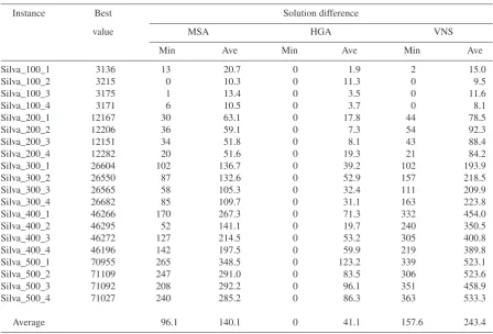
Table 1 summarizes the results of MSA, HGA and VNS on the Silva instances. Each entry of the dissimilarity matrix defining an instance in this se-ries is an integer randomly and uniformly drawn from the interval[0,9]. The number of elementsn∈
{100,200,300,400,500}is included in the name of an instance (first column in the table). For example,
Silva_100_1 denotes the first (out of four) instance with 100 elements. The numerical experiment was conducted for the case where the number of groupsm was fixed at 10. The size of each group was bounded from below by a = 0.8n/m and from above by b= 1.2n/m. The second column of Table 1 contains, for each instance, the value of the best solution ob-tained from all runs of MSA, HGA and VNS. The third (respectively, fourth) column shows the differ-ence between the value displayed in the second col-umn and the value of the best solution out of 10 runs (respectively, the average value of 10 solutions) found
by MSA. The remaining columns give these differ-ences for HGA and VNS. The results, averaged over all problem instances, are presented in the last row of the table.
As seen in Table 1, HGA is definitely superior to both the MSA and VNS algorithms. Basically, the solutions found by HGA appear to be the best in our experiment. Compared with the results of HGA, the MSA and VNS algorithms tie in one and, respec-tively, three cases and produce inferior solutions in all other cases. We can also see from Table 1 that VNS performs better than MSA for instances of size 100 but is worse than MSA for all larger instances in the dataset. Overall, the ranking of the results from best to worst is as follows: "MinHGA", "AveHGA", "Min
MSA", "AveMSA", "MinVNS", and "AveVNS". In Table 2 we show the results obtained for the
Duarte-Martíinstances. All the entriesdijof the dis-similarity matrix D for these instances are integers generated randomly from a uniform distribution be-tween 0 and 10. We should mention that Duarte and Martí have generated 20 dissimilarity matrices of size 2000×2000. We present the results for the first 10 of them. The results of MSA, HGA and VNS for the other 10 matrices are very similar to those reported in Table 2. For our experimentation, we have fixed the number of groups to 50, the minimum group size to 0.8n/m = 32, and the maximum group size to 1.2n/m= 48. The structure of Table 2 is the same as that of Table 1.
From Table 2, we find that, according to solution quality, the algorithms can be ranked in the reverse or-der of that observed in the experiment with theSilva
instances. Now VNS is the best-performing algorithm of the three. Meanwhile, the HGA algorithm shows the worst performance. After analyzing the results of the experiment, we found out that the LS procedure was quite time consuming for the Duarte-Martí in-stances, especially when applied to a solution that is far from local optima. This is probably the main rea-son why the performance of HGA deteriorates sig-nificantly on large-size instances. When applied to
DM_1, for example, HGA was able to invoke the LS procedure within the allotted one hour only 332 times on the average (excluding the calls to LS throughout the construction of the initial population). For com-parison, the average number of LS invocations in the case of the Silva_500_1instance exceeded 688000. When solvingDM_1by the VNS algorithm, the aver-age number of calls to LS was 1748.
We do not present the results of the pure genetic algorithm, which is obtained from HGA by deleting Step 4 (see Section 3) where hybridization with local search occurs. The pure GA generates a huge
Instance Best Solution difference
value MSA HGA VNS
Min Ave Min Ave Min Ave
Silva_100_1 3136 13 20.7 0 1.9 2 15.0
Silva_100_2 3215 0 10.3 0 11.3 0 9.5
Silva_100_3 3175 1 13.4 0 3.5 0 11.6
Silva_100_4 3171 6 10.5 0 3.7 0 8.1
Silva_200_1 12167 30 63.1 0 17.8 44 78.5
Silva_200_2 12206 36 59.1 0 7.3 54 92.3
Silva_200_3 12151 34 51.8 0 8.1 43 88.4
Silva_200_4 12282 20 51.6 0 19.3 21 84.2
Silva_300_1 26604 102 136.7 0 39.2 102 193.9
Silva_300_2 26550 87 132.6 0 52.9 157 218.5
Silva_300_3 26565 58 105.3 0 32.4 111 209.9
Silva_300_4 26682 85 109.7 0 31.1 163 223.8
Silva_400_1 46266 170 267.3 0 71.3 332 454.0
Silva_400_2 46295 52 141.1 0 19.7 240 350.5
Silva_400_3 46272 127 214.5 0 53.2 305 400.8
Silva_400_4 46196 142 197.5 0 59.9 219 389.8
Silva_500_1 70955 265 348.5 0 123.2 339 523.1
Silva_500_2 71109 247 291.0 0 83.5 306 523.6
Silva_500_3 71092 208 292.2 0 96.1 351 458.9
Silva_500_4 71027 240 285.2 0 86.3 363 533.3
Average 96.1 140.1 0 41.1 157.6 243.4
Table 2. Results of running MSA, HGA and VNS on theDuarte-Martíinstances (n= 2000,m= 50,a= 32,
b= 48)
Instance Best Solution difference
value MSA HGA VNS
Min Ave Min Ave Min Ave
DM_1 269990 1160 1424.4 2665 2823.7 0 588.8
DM_2 270409 1509 1877.9 3060 3246.3 0 908.1
DM_3 269710 768 1121.7 2382 2559.6 0 460.1
DM_4 269790 430 1135.5 2053 2507.4 0 644.1
DM_5 269675 495 1175.1 1983 2455.8 0 365.7
DM_6 269933 877 1225.7 2537 2772.8 0 553.5
DM_7 269781 952 1275.8 2405 2705.8 0 558.9
DM_8 270325 1535 1833.4 2718 3050.6 0 748.5
DM_9 269830 866 1209.8 2357 2565.5 0 535.1
DM_10 269892 1106 1417.9 2447 2643.3 0 547.4
Average 969.8 1369.7 2460.7 2733.1 0 591.0
ber of offspring, but each of them is worse than its own parents. This is because the parents are sampled from the initial population which is built using the lo-cal search procedure. The mating mechanism (Step 3 in the description of HGA) is too weak to be able to
produce an offspring that could outperform the fitness of its parents. Thus the performance of the pure GA is poor compared with the described MSA, HGA and VNS implementations.
6. Conclusions
In this paper we have presented simulated an-nealing (MSA), hybrid genetic (HGA) and variable neighborhood search (VNS) algorithms for the max-imally diverse grouping problem. In order to evalu-ate the performance of these algorithms we conducted computational experiments on two sets of problem instances of size up to 2000 elements. The results show that neither of the algorithms is a clear win-ner in all cases. For smaller instances, the best results were achieved using HGA. However, the comparison of the heuristics on larger MDGP instances favors the VNS algorithm. In both cases, MSA is the second best method. Certainly some more experiments, especially by varying group size, could be run to better evaluate the potential of various approaches.
In an additional experiment, we let HGA and VNS run for longer on a number of problem instances in the datasets we have used. The result was that in all cases except for theSilva_100_2andSilva_100_3 in-stances the solutions obtained were better than those reported in Tables 1 and 2. This means that there is some room for improvements and further research on the heuristics for solving the MDGP. For example, different mating mechanism in HGA and various lo-cal search procedures both in HGA and VNS could be tried. Also, the development of new algorithms for the MDGP, based on other metaheuristics than those considered in this paper, is an important line of future work.
References
[1] T. Arani, V. Lotfi. A three phased approach to final exam scheduling.IIE Transactions, 1989,Vol.21, 86– 96.
[2] K.R. Baker, S.G. Powell. Methods for assigning stu-dents to groups: a study of alternative objective func-tions. Journal of the Operational Research Society, 2002,Vol.53, 397–404.
[3] J. Brimberg, N. Mladenovi´c, D. Uroševi´c, E. Ngai. Variable neighborhood search for the heaviest k -subgraph. Computers and Operations Research, 2009,Vol.36, 2885–2891.
[4] Y. Chen, Z.-P. Fan, J. Ma, S. Zeng. A hybrid group-ing genetic algorithm for reviewer group construction problem. Expert Systems with Applications, 2011, Vol.38, 2401–2411.
[5] A. Duarte, R. Martí. Tabu search and GRASP for the maximum diversity problem. European Journal of Operational Research, 2007,Vol.178, 71–84. [6] Z.P. Fan, Y. Chen, J. Ma, S. Zeng. A hybrid genetic
algorithmic approach to the maximally diverse group-ing problem.Journal of the Operational Research So-ciety, 2011,Vol.62, 1423–1430.
[7] P. Hansen, N. Mladenovi´c. Variable neighborhood search: principles and applications.European Journal of Operational Research, 2001,Vol.130, 449–467. [8] P. Hansen, N. Mladenovi´c, J.A. Moreno Pérez.
Variable neighbourhood search: methods and applica-tions.4OR, 2008,Vol.6, 319–360.
[9] P. Hansen, N. Mladenovi´c, J.A. Moreno Pérez. Variable neighbourhood search: methods and ap-plications. Annals of Operations Research, 2010, Vol.175, 367–407.
[10] V. Lotfi, R. Cerveny. A final-exam-scheduling pack-age. Journal of the Operational Research Society, 1991,Vol.42, 205–216.
[11] R. Martí, M. Gallego, A. Duarte. Maximum di-versity problem. http://www.optsicom.es/mdp/. Ac-cessed 25 May 2011.
[12] R. Martí, M. Gallego, A. Duarte, E.G. Pardo. Heuristics and metaheuristics for the maximum diver-sity problem. Journal of Heuristics, 2011, in press, DOI: 10.1007/s10732-011-9172-4.
[13] J. Mingers, F.A. O’Brien. Creating student groups with similar characteristics: a heuristic approach. Omega, 1995,Vol.23, 313–321.
[14] G. Palubeckis. Iterated tabu search for the maximum diversity problem.Applied Mathematics and Compu-tation, 2007,Vol.189, 371–383.
[15] G. Palubeckis. A new bounding procedure and an improved exact algorithm for the Max-2-SAT prob-lem. Applied Mathematics and Computation, 2009, Vol.215, 1106–1117.
[16] G. Palubeckis, D. Rubliauskas, A. Targamadz˙e. Metaheuristic approaches for the quadratic minimum spanning tree problem. Information Technology and Control, 2010,Vol.39, 257–268.
[17] G.C. Silva, L.S. Ochi, S.L. Martins. Experimen-tal comparison of greedy randomized adaptive search procedures for the maximum diversity problem. Lec-ture Notes in Computer Science, 2004,Vol.3059, 498– 512.
[18] R.R. Weitz, M.T. Jelassi. Assigning students to groups: a multi-criteria decision support system ap-proach.Decision Sciences, 1992,Vol.23, 746–757. [19] R.R. Weitz, S. Lakshminarayanan. On a heuristic
for the final exam scheduling problem.Journal of the Operational Research Society, 1996,Vol.47, 599–600. [20] R.R. Weitz, S. Lakshminarayanan. An empirical comparison of heuristic and graph theoretic methods for creating maximally diverse groups, VLSI design, and exam scheduling.Omega, 1997,Vol.25, 473–482. [21] R.R. Weitz, S. Lakshminarayanan. An empirical comparison of heuristic methods for creating maxi-mally diverse groups. Journal of the Operational Re-search Society, 1998,Vol.49, 635–646.
[22] H.K. Yeoh, M.I.M. Nor. An algorithm to form balanced and diverse groups of students. Com-puter Applications in Engineering Education, 2011, Vol.19, 582–590.