A new panel dataset for cross country analyses of national systems, growth and development (CANA)

(1)

Munich Personal RePEc Archive

A new panel dataset for cross-country

analyses of national systems, growth and

development (CANA)

Castellacci, Fulvio and Natera, Jose Miguel

January 2011

Online at

https://mpra.ub.uni-muenchen.de/28376/

(2)

A new panel dataset for cross-country analyses

of national systems, growth and development

(CANA)

Fulvio Castellacci

*

and Jose Miguel Natera

†

*

Norwegian Institute of International Affairs (NUPI), Oslo, Norway. E-mail: [email protected]

†

University Complutense, Madrid, Spain. E-mail: [email protected]

NUPI Working Paper, January 2011

Abstract

Missing data represent an important limitation for cross-country analyses of national systems, growth and development. This paper presents a new cross-country panel dataset with no missing value. We make use of a new method of multiple imputation that has recently been developed by Honaker and King (2010) to deal specifically with time-series cross-section data at the country-level. We apply this method to construct a large dataset containing a great number of indicators measuring six key country-specific dimensions: innovation and technological capabilities, education system and human capital, infrastructures, economic competitiveness, political-institutional factors, and social capital. The CANA panel dataset thus obtained provides a rich and complete set of 41 indicators for 134 countries in the period 1980-2008 (for a total of 3886 country-year observations). The empirical analysis shows the reliability of the dataset and its usefulness for cross-country analyses of national systems, growth and development. The new dataset is publicly available.

The CANA database can be downloaded at the web address:

http://english.nupi.no/Activities/Projects/CANA

Please contact the authors for any question, or suggestion for future improvements.

(3)

“If you torture the data long enough, Nature will confess” (Ronald Coase, 1982)

1. Introduction

A recent strand of research within the national systems literature investigates the

characteristics of NIS in developing countries and their relevance for economic growth

and competitiveness (Lundvall et al., 2009). Some of this applied research makes use of

available statistical data for large samples of countries and carries out quantitative studies

of the economic and social capabilities of nations and the impacts of these on the growth

and development process (Archibugi and Coco, 2004; Fagerberg et alia, 2007; Castellacci

and Archibugi, 2008).

This empirical research faces however one important limitation: the problem of missing

data. This problem, and the related consequences and possible solutions, have not been

adequately studied yet in the literature. The missing data problem arises because many of

the variables that are of interest for measuring the characteristics and evolution of national

systems are only available for a restricted sample of (advanced and middle-income)

economies and for a limited time span only.

As a consequence, cross-country analyses in this field are typically forced to take a hard

decision: either to focus on a restricted country sample for a relatively long period of time,

or to focus on a very short time span for a large sample of economies. Both alternatives

are problematic: the former neglects the study of NIS in developing and less developed

economies, whereas the latter neglects the study of the dynamics and evolution of national

systems over time.

This paper proposes a third alternative that provides a possible solution to this trade off:

the use of multiple imputation methods to estimate missing data and obtain a complete

panel dataset for all countries and the whole period under investigation. Multiple

imputation methods represent a modern statistical approach that aims at overcoming the

missing data problem (Rubin, 1987). This methodology has received increasing attention

in the last decade and has been applied in a number of different fields of research. In

particular, Honaker and King (2010) have very recently proposed a new multiple

imputation algorithm that is specifically developed to deal with time-series cross-section

data at the country-level.

Our paper employs this new method of multiple imputation and shows its relevance for

(4)

new panel dataset (CANA) that contains no missing value. The dataset comprises 41

indicators measuring six key country-specific dimensions: innovation and technological

capabilities, education system and human capital, infrastructures, economic

competitiveness, political-institutional factors, and social capital. The CANA panel

dataset that is obtained by estimating the missing values in the original data sources

provides rich and complete statistical information on 134 countries for the entire period

1980-2008 (for a total of 3886 country-year observations). Our empirical analysis of this

dataset shows its reliability and points out its usefulness for future cross-country studies of

national systems, growth and development. We make the new dataset publicly available

on the web.

The paper is organized as follows. Section 2 briefly reviews the literature and discusses

the missing data problem. Section 3 introduces Honaker and King’s (2010) new method of

multiple imputation. Section 4 presents the CANA dataset and indicators and carries out a

descriptive analysis of some of its key characteristics. Section 5 provides an analysis of

the reliability of the new data material obtained through multiple imputation. Section 6

concludes by summarizing the main results and implications of the paper. A

methodological Appendix contains all more specific details regarding the database

construction, characteristics and quality assessment.

2. Cross-country analyses of national systems, growth and development:

the problem of missing data

The national innovation system (NIS) perspective originally developed during the 1990s

to understand the broad set of factors shaping the innovation and imitation ability of

countries, and how these factors could contribute to explain cross-country differences in

economic growth and competitiveness (Lundvall, 1992; Edquist, 1997). Empirical studies

in this tradition initially focused mostly on advanced economies in the OECD area

(Nelson, 1993). However, the NIS literature has recently shifted the focus towards the

empirical study of innovation systems within the context of developing and less developed

economies (Lundvall et alia,, 2009).1

1

(5)

A well-known challenge for applied research in this field is how to operationalize the

innovation system theoretical view in empirical studies and, relatedly, how to measure the

complex and multifaceted concept of national innovation system and its relationship to

countries’ economic performance. Quantitative applied studies of NIS and development

have so far made use of two different (albeit complementary) approaches.

The first approach is rooted in the traditional literature on technology and convergence

(Abramovitz, 1986; Verspagen, 1991; Fagerberg, 1994). Following a technology-gap

Schumpeterian approach, recent econometric studies have focused on a few key variables

that explain (or summarize) cross-country differences in the innovation ability of

countries as well as their different capabilities to imitate foreign advanced knowledge, and

then analysed the empirical relationship between these innovation and imitation factors

and cross-country differences in GDP per capita growth (Fagerberg and Verspagen, 2002;

Castellacci, 2004, 2008 and 2011; Fagerberg et alia, 2007). Since one main motivation of

this type of studies is to analyse the dynamics and evolution of national systems in a

long-run perspective, they typically consider a relatively long time span (e.g. from the 1970s or

1980s onward), but must for this reason focus on a more restricted sample of countries

(e.g. between 70 and 90 countries). Due to the lack of statistical data for a sufficiently

long period of time, therefore, a great number of developing economies and the vast

majority of less developed countries are neglected by this type of cross-country studies.

The second approach is based on the construction and descriptive analysis of composite

indicators. In a nutshell, this approach recognizes the complex and multidimensional

nature of national systems of innovation and tries to measure some of their most important

characteristics by considering a large set of variables representing distinct dimensions of

technological capabilities, and then combining them together into a single composite

indicator – which may be interpreted as a rough summary measure of a country’s relative

position vis-a-vis other national systems. Desai et alia (2002) and Archibugi and Coco

(2004) have firstly proposed composite indicators based on a simple aggregation (simple

or weighted averages) of a number of technology variables. Godinho et alia (2005),

Castellacci and Archibugi (2008) and Fagerberg and Srholec (2008) have then considered

a larger number of innovation system dimensions and analysed them by means of factor

and cluster analysis techniques. As compared to the first approach, the composite

indicator approach has a more explicit focus on the comparison across a larger number of

countries. Consequently, due to the lack of data availability on less developed countries

(6)

time span (i.e. a cross-section description of the sample in one point in time, e.g. the

1990s and/or the 2000s).

Considering the two approaches together, it is then clear that researchers seeking to carry

out quantitative analyses of innovation systems and development commonly face a

dilemma with respect to the data they decide to use. Either, they can focus on a small

sample of (mostly advanced and middle-income) economies over a long period of time –

or conversely they can study a much larger sample of countries (including developing

ones) for carrying out a shorter run (static) type of analysis. Such a dilemma is of course

caused by the fact that, for most variables that are of interest for measuring and studying

innovation systems, the availability of cross-section time-series (panel) data is limited:

data coverage is rather low for many developing economies for the years before 2000, and

it improves substantially as we move closer to the present.

Both solutions that are commonly adopted by applied researchers to deal with this

dilemma, however, are problematic. If the econometric analysis focuses on the dynamic

behaviour of a restricted sample of economies, as typically done in the technology-gap

tradition, the parameters of interest that are estimated through the standard cross-country

growth regression are not representative of the whole world economy, and do not provide

any information about the large and populated bunch of less developed countries. In

econometric terms, the regression results will provide a biased estimation of the role of

innovation and imitation capabilities. Relatedly, by removing most developing countries

observations from the sample under study (e.g. by listwise deletion), this regression

approach tends to be inefficient as it disregards the potentially useful information that is

present in the variables that are (at least partly) available for developing countries.

By contrast, if the applied study decides to consider a much larger sample of countries

(including developing ones), as it is for instance the case in the composite indicator

approach, the analysis inevitably assumes a static flavour and largely neglects the

dynamic dimension. This is indeed unfortunate, since it was precisely the study of the

dynamic evolution of national systems that represented one of the key motivation

underlying the development of national systems theories.

Surprisingly, such a dilemma – and the possibly problematic consequences of the

solutions that are typically adopted in this branch of applied research – have not been

properly investigated yet in the literature. This paper intends to contribute to this issue by

pointing out a possible solution to the trade-off mentioned above. We construct and make

(7)

the original data sources are estimated by means of a statistical approach that is known as

multiple imputation (Rubin, 1987). Multiple imputation methods for missing data analysis

have experienced a rapid development in the last few years and have been increasingly

applied in a wide number of research fields. The next section will introduce this statistical

method in the context of time-series cross-section data.

3. The multiple imputation method

Multiple imputation methods were firstly introduced two decades ago by Rubin (1987).

They provide an appropriate and efficient statistical methodology to estimate missing

data, which overcomes the problems associated with the use of listwise deletion or other

ad hoc procedures to fill in missing values in a dataset. The general idea and intuition of

this approach can be summarized as follows (see overviews in Rubin, 1996; Schafer and

Olsen, 1998; Horton and Kleinman, 2007).

Given a dataset that comprises both observed and missing values, the latter are estimated

by making use of all available information (i.e. the observed data). This estimation is

repeated m times, so that m different complete datasets are generated (reflecting the

uncertainty regarding the unknown values of the missing data). Finally, all subsequent

econometric analyses that the researcher intends to carry out will be repeated m times, one

for each of the estimated datasets, and the multiple results thus obtained will be easily

combined together in order to get to a final value of the scientific estimand of interest (e.g.

a set of regression coefficients and their significance levels).

Within this general statistical approach, Honaker and King (2010) have very recently

introduced a novel multiple imputation method that is specifically developed to deal with

time-series cross-section data (i.e. panels). This type of data has in the last few years been

increasingly used for cross-country analyses in the fields of economic growth and

development, comparative politics and international relations. However, missing data

problems introduce severe bias and efficiency problems in this type of studies, as pointed

out in the previous section. Honaker and King’s (2010) method is particularly attractive

because its multiple imputation algorithm efficiently exploits the panel nature of the

dataset and makes it possible, among other things, to properly take into account the issue

of cross-country heterogeneity by introducing fixed effects and country-specific time

(8)

Suppose we have a latent data matrix X, composed of p variables (columns) and n

observations (rows). Each element of this matrix, xijt, represents the value of country i for

variable j at time t. The data matrix is composed of both observed and missing values:

X = {XOBS; XMIS}. In order to rectangularize the dataset, we define a missingness matrix

M such that each of its elements takes value 1 if it is missing and 0 if it is an observed

value. We then apply the simple matrix transformation: XOBS = X * (1 – M), so that our

matrix dataset will now contain 0s instead of missing values (for further details on this

framework, see Honaker and King, 2010, p. 576).

Multiple imputation methods typically make two general assumptions on the data

generating process. The first is that X is assumed to have a multivariate normal

distribution: X ~ N (μ; Σ), where μ and Σ represent the (unknown) parameters of the

Gaussian (mean and variance). The useful implication of assuming a normal distribution

is that each variable can be described as a linear function of the others.2

The second is the so-called missing at random (MAR) assumption. This means that M can

be predicted by XOBS but not by XMIS (after controlling for XOBS), i.e. formally:

P (M | X) = P (M | XOBS). The MAR assumption implies that the statistical relationship

(e.g. regression coefficient) between one variable and another is the same for the groups

of observed and missing observations. Therefore, we can use this relationship as estimated

for the group of observed data in order to impute the missing values (Shapen and Olsen,

1998; Honaker and King, 2010). This condition also suggests that all the variables that are

potentially relevant to explain the missingness pattern should be included in the

imputation model.3

The core of Honaker and King’s (2010) new multiple imputation method is the

specification of the estimation model for imputing the missing values in the dataset:

xijMIS = βj xi;-jOBS + γj t + δij + δij t + εij (1)

where xijMIS are the missing values to be estimated, for observation i and variable j, and

xi;-jOBS are all other observed values for observation i and all variables excluding j (we

2

The statistical literature on multiple imputation methods has shown that departures from the normality assumption are not problematic and do not usually introduce any important bias in the imputation model.

3

(9)

have for simplicity omitted the time index t). The parameter βj represents the estimate of

the cross-sectional relation between the variable j and the set of covariates – j; γj is an

estimate of the time trend; δij is a set of individual fixed effects; δij t is an interaction term

between the time trend and the fixed effects, which provides an estimate of the

country-specific time trends (i.e. a different time trend is allowed for each observation); finally, εij

is the error term of the model.4 For clarity of exposition, it is useful to rewrite this model

in its extended form:

xi1MIS = β1 xi;-1OBS + γ1 t + δi1 + δi1 t + εi1

...

xipMIS = βp xi;-pOBS + γp t + δip + δip t + εip (2)

The formulation in (2) makes clear that our imputation model is composed of p equations,

one for each variable of the model. Each variable is estimated as a linear function of all

the others. In each of these p equations, missing values for a given variable are estimated

as a function of the observed values for all the other variables.

The model is estimated through the so-called EM algorithm. This is an iterative algorithm

comprising two steps. In the first (E-step), missing values are replaced by their conditional

expectation (obtained through the estimation of (2)) – given the current estimate of the

unknown parameters μ and Σ. In the second (M-step), a new estimate of the parameters μ

and Σ is calculated from the data obtained in the first step. The two steps are iteratively

repeated until the algorithm will converge to a final solution.

As pointed out above, the key idea common to all multiple imputation methods is that the

imputation process is repeated m times, so that m distinct complete datasets are eventually

obtained – reflecting the uncertainty regarding the unknown values of the missing data.5

Honaker and King’s method implements this idea by setting up the following bootstrap

procedure: m samples of size n are drawn with replacement from the data X; in each of

4

For simplicity, the model specification in equation 1 assumes a linear trend for all variables and all observations. Honaker and King’s method, however, makes it also possible to specify more complex non-linear adjustment processes in order to achieve a better fit of the estimated series to the observed data.

5

(10)

these m samples, the EM algorithm described above is run to obtain μ, Σ and the complete

dataset. Thus, m complete datasets are obtained ready for the subsequent analyses.6

In summary, this new multiple imputation method presents two main advantages. First,

similarly to other related methods, it avoids bias and efficiency problems related to the

presence of missing values and/or the use of ad hoc methods to dealing with them (e.g.

listwise deletion). Secondly, it is specifically developed to deal with time-series

cross-section data. In particular, it is well-suited to deal with the issue of cross-country

heterogeneity, since it allows for both country fixed effects as well as country-specific

time trends.

Despite these attractive features, it is however important to emphasize that this type of

missing data estimation procedures should be applied with caution. Specifically, when the

percentage of missing data is high, the imputation procedure tends to be less precise and

reliable, and it is therefore important to carefully scrutinize the results. We will discuss

this important issue in section 5 and provide all related details in the Appendix.

4. A new panel dataset (CANA)

We now present the main characteristics of the CANA panel dataset, which has been

constructed by applying the method of multiple imputation described in the previous

section. The complete dataset that we have obtained contains information for a large

number of relevant variables, and for a very large panel of countries. Specifically, for 34

indicators we have obtained complete data for 134 countries for the whole period

1980-2008 (3886 country-year observations); for seven other indicators we have instead

achieved a somewhat smaller country coverage (see details below). On the whole, this

new dataset represents a rich statistical material to carry out cross-country analyses of

national systems, of their evolution in the last three decades, and of the relationships of

these characteristics to countries’ social and economic development.

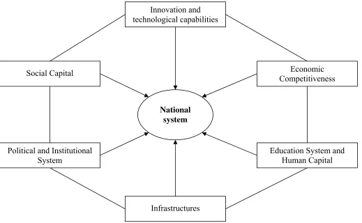
Given that the concept of national systems is complex, multifaceted and comprising a

great number of relevant factors interacting with each other, our database adopts a broad

and multidimensional operationalization of it. Our stylized view, broadly in line with the

6

(11)

previous literature, is presented in figure 1.7 We represent national systems as composed

of six main dimensions: (1) Innovation and technological capabilities; (2) Education and

human capital; (3) Infrastructures; (4) Economic competitiveness; (5) Social capital; (6)

Political and institutional factors. The underlying idea motivating the construction of this

database is that it is the dynamics and complex interactions between these six dimensions

that represent the driving force of national systems’s social and economic development,

and it is therefore crucial for empirical analyses in this field to have availability of

statistical information for an as large as possible number of indicators and country-year

observations.8

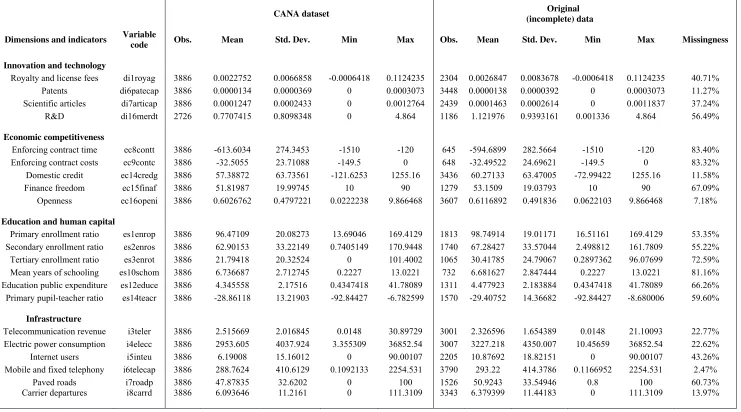
Table 1 presents a list of the 41 indicators included in the CANA database, and compares

some descriptive statistics of the new (complete) panel dataset with those of the

corresponding variables in the original (incomplete) data sources. The last column of the

table shows the share of missing data present in the original data sources, which is in

many cases quite high. A comparison of the left and right-hand sides of the table indicates

that the descriptive statistics of the complete version of the data (containing no missing

value) are indeed very close to those of the original sources – which gives a first and

important indication of the quality and reliability of the new CANA dataset (this aspect

will be analysed in further details in the next section).

< Figure 1 and table 1 here >

The methodology that we have followed to construct the complete dataset and indicators

has proceeded in four subsequent steps (see figure A1 in the Appendix). In the first, we

have collected a total number of 55 indicators from publicly available databases and a

variety of different sources (see the Appendix for a complete list of indicators and data

sources). This large set of indicators covers a wide spectrum of variables that are

potentially relevant to measure the six country-specific dimensions pointed out above.

This initial dataset contains as well-known a great number of missing values for many of

the countries and the variables of interest. In the remainder of the paper, we will for

simplicity refer to it as the observed (or the original) dataset.

7

Other empirical exercises in the NIS literature have previously made use of (at least some of) these dimensions and indicators. See in particular Godinho et alia (2005), Castellacci and Archibugi (2008) and Fagerberg and Srholec (2008).

8

(12)

In the second step, we have run Honaker and King’s (2010) multiple imputation procedure

as described in section 4 above. We have carried out the imputation algorithm for each of

the six dimensions separately.9 In order to achieve a high efficiency level, we have set m

= 15, i.e. fifteen complete datasets have been estimated for each of the six dimensions. We

have then combined these fifteen datasets into a single one, which is our complete CANA

dataset. This is a rich rectangular matrix containing information for all relevant variables

for 3886 observations (134 economies for the whole period 1980-2008).

Thirdly, we have carried out a thorough evaluation of each of these 55 variables in order

to analyse the quality of the imputed data and the extent to which the new complete

dataset may be considered a good and reliable extension of the original data sources. This

evaluation process is discussed in details in the next section. In short, the main result of

this assessment work is that the multiple imputation method has been successful for 34

indicators, which we have then included in the final version of database for the whole

range of 3886 country-year observations (134 countries).

Fourthly, in the attempt to increase the number of “accepted” indicators, we have repeated

the imputation procedure for all the remaining indicators and for a smaller number of

countries – i.e. excluding those countries that have a very high share of missing data in the

original sources. After a careful quality check of this second round of multiple

imputations, we have decided to include seven more indicators in the final version of the

CANA database: R&D (for 94 countries) and six social capital variables (for 80

countries).

In summary, the final version of the CANA database that we make available contains a

total number of 41 indicators (34 with full country coverage and seven for a smaller

sample), whereas the remaining 14 indicators have been rejected and not included in the

database because the results of the imputation procedure has not led to imputed data of a

sufficiently good and reliable quality.

A simple descriptive analysis of the CANA dataset and indicators illustrates the relevance

and usefulness of this new data material to gain new empirical insights on some of the

main characteristics of national systems in such a broad cross-section of countries, and

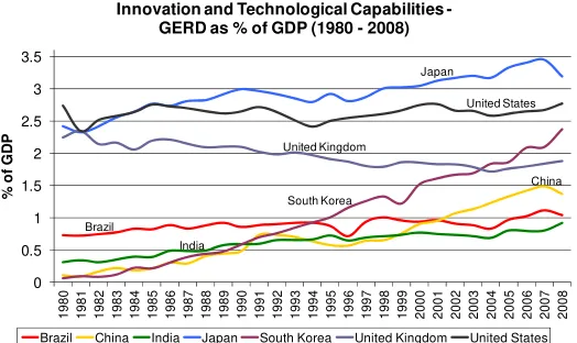
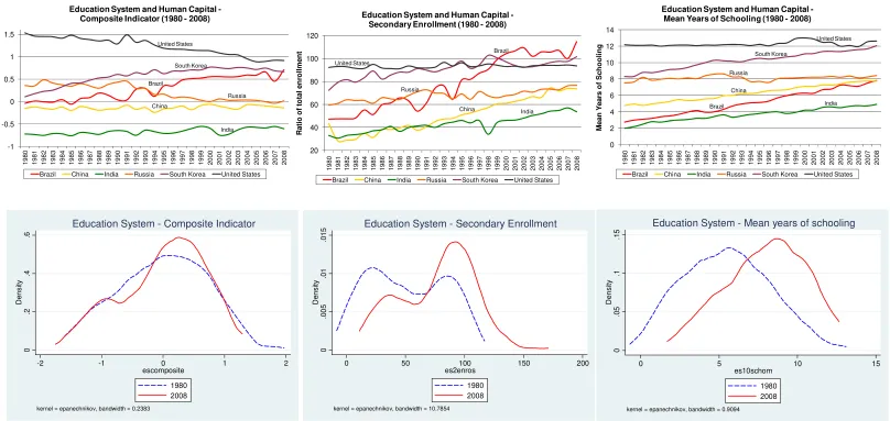
particularly on their dynamic processes over the period 1980-2008. Figures 2 to 7 show

9

(13)

the time path of some of the key variables of interest. For each of the six dimensions, we

also report a composite indicator and its time trend. The composite indicators, calculated

for illustrative purposes only, have been obtained by first standardizing all the variables

included in a given dimension (and for any given year), and then calculating a simple

average of them. The upper part of figures 2 to 7 depicts the time trend for some selected

countries, whereas the lower part plots the cross-country distribution of each dimension at

the beginning and the end of the period (1980 and 2008). In each figure, we report the

composite indicator on the left-hand panel, and two of the selected indicators used to

construct it on the middle and right-hand panels.

Figure 2 focuses on countries’ innovation and technological capabilities. The lower part of

the figure shows that the cross-country distribution of innovative capabilities has not

changed substantially over the period, indicating that no significant worldwide

improvement has taken place in this dimension (Castellacci, 2011). However, the pattern

is somewhat different for the R&D variable, since this focuses on a smaller number of

countries. The upper part of the figure suggests that the technological dynamics process

has been far from uniform and that different countries have experienced markedly

different trends. In particular, the US and Japan are the leading economies that have

experienced the most pronounced increase over time, whereas South Korea and China are

the followers that have experienced the most rapid technological catching up process.

Most other middle-income and less developed economies have not been able to catch up

with respect to this dimension.

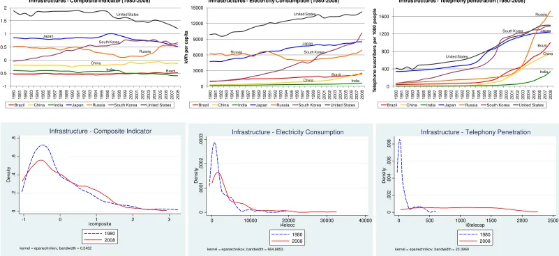
A worldwide and relatively rapid process of convergence is instead more apparent when

we shift the focus to figures 3 and 4, which study the evolution of the human capital and

infrastructures dimensions respectively. The kernel densities reported in the lower part of

these figures show that the cross-country distributions of these two dimensions have

visibly shifted towards the right, thus indicating an overall improvement of countries’

education system and infrastructure level. The time path for some selected economies

reported in the upper part of these figures also show the rapid catching up process

experienced by some developing countries (and many others not reported in these graphs)

with respect to these dimensions.

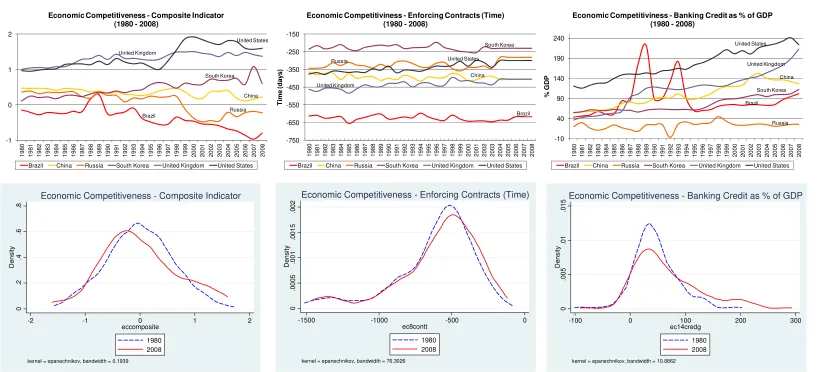
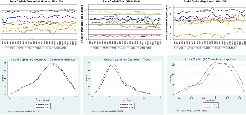
As for the remaining three dimensions – economic competitiveness (figure 5), social

capital (figure 6) and political-institutional factors (figure 7) – the worldwide pattern of

evolution over time is less clear-cut and depends on the specific indicators that we take

(14)

indicator of happiness has on average increased over time, whereas the trust variable has

not.

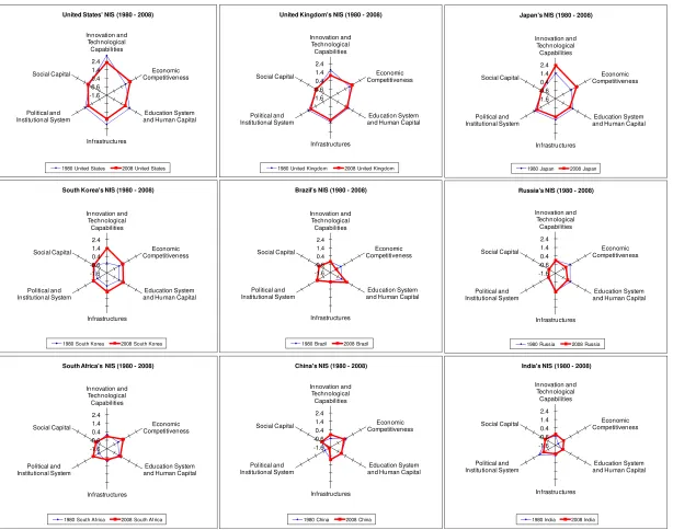
In order to provide a more synthetic view of the main patterns and evolution of NIS,

figure 8 shows a set of radar graphs for some selected countries: four technologically

advanced economies (US, UK, Japan, South Korea) plus the BRICS countries (Brazil,

Russia, India, China and South Africa). For each country, the standardized value of each

composite indicator is reported for both the beginning and the end of the period (1980 and

2008), so that these radar graphs provide a summary view of some key characteristics of

NIS and their dynamic evolution in the last three decades. The graphs are rather

informative. More advanced countries have on average a much greater surface than the

catching up BRICS economies, indicating an overall greater level of the set of relevant

technological, social and economic capabilities. Japan and South Korea are those that

appear to have improved their relative position more visibly over time. By contrast, within

the group of BRICS countries, the catching up process between the beginning and the end

of the period has been more striking for China, Brazil and South Africa, and less so for

Russia and India. It is however important to emphasize that the dynamics looks somewhat

different for each of the six dimensions considered in figure 8, so that our summary

description here is only done for illustrative purposes.

The descriptive analysis of cross-country patterns and evolution that has been briefly

presented in this section will be extended and refined in a number of ways in future

research. However, as previously pointed out, our purpose here is not to carry out a

complete and detailed analysis of the characteristics and evolution of national systems, but

rather to provide a simple empirical illustration of the usefulness of the new CANA panel

dataset, and of how it can be used for cross-country studies of national systems and

development.

(15)

5. An analysis of the reliability of the CANA dataset and indicators

The illustration presented in the previous section has shown some of the advantages of

adopting a method of multiple imputation to estimate missing values and obtain a rich

complete dataset for the cross-country empirical investigation of national systems and

development. However, at the same time as emphasizing the usefulness of the CANA

dataset and indicators that we have constructed, it is also important to assess the quality of

this newly obtained data material and investigate the possible limitations of the multiple

imputation method that has been used to construct it.

As mentioned in the previous section, during the construction of the CANA database we

have initially collected a total number of 55 indicators, which are intended to measure six

different dimensions of countries’ social, institutional and economic development. We

have then carried out a first main round of multiple imputations in order to estimate the

missing values in the original sources. After this first set of imputation estimations, we

have carried out a thorough evaluation of each of these 55 variables in order to analyse the

quality of the imputed data and the extent to which the new complete dataset may be

considered a good and reliable extension and estimation of the original data sources. We

have concluded that the multiple imputation method has been successful for 34 indicators,

which we have then included in the final version of database for the whole range of 3886

country-year observations (134 countries).

Next, in the attempt to increase the number of “accepted” (reliable) indicators included in

the dataset, we have repeated the imputation procedure for all the remaining indicators

and for a smaller number of countries – i.e. excluding those countries that have a very

high share of missing data in the original sources. After a second round of quality and

reliability check, we have decided to include seven more indicators in the final version of

the CANA database: R&D (for 94 countries) and six social capital variables (for 80

countries). Therefore, the final version of the CANA database contains a total number of

41 indicators (34 with full country coverage and seven for a smaller sample), whereas the

remaining 14 indicators have been rejected and not included in the database because the

results of the imputation procedure has not led to imputed data of a sufficiently good and

reliable quality.

In order to illustrate our data assessment procedure and the reliability of the indicators that

we have included in the final version of the database, we summarize the main steps here

and report further material in the Appendix (see section A.3). Our evaluation process has

(16)

versus the original data; (2) a graphical inspection of their kernel density graphs; (3) a

comparison of the respective correlation tables.

First, table 1 (see previous section) reports a comparison of the main descriptive statistics

for the CANA (complete) dataset versus the observed (original) data sources. The table

shows that, for the 41 indicators included in the final version of the database, the means of

the two distributions are rather similar in nearly all cases. On average, the means are

however slightly lower for the complete version of the dataset, since this includes data for

a larger number of developing economies that is only partly available in the original

datasets.

A second and more detailed assessment exercise is reported in figure A2 (see the

Appendix). The various graphs in figure A2 compare the statistical distributions (kernel

densities) of the observed and the complete datasets for all the 41 indicators that we have

included in the final version of the CANA database. As previously specified, the observed

dataset is the original database that we have constructed by combining together indicators

from different publicly available data sources (i.e. the one containing missing values for

some of the variables and some of the country-year observations), whereas the complete

dataset is the one that we have obtained by estimating missing values through Honaker

and King’s (2010) multiple imputation procedure.

The idea of comparing the two distributions is to provide an easy and effective visual

inspection of the reliability of the multiple imputation results: if the statistical distribution

of the complete dataset is substantially the same (or very similar to) the one for the

observed data, we may be confident about the quality and reliability of the imputation

results; by contrast, if the two distributions turn out to be quite different from each other,

this would imply that the new data that have been estimated depart substantially from the

original ones, and hence the results of the multiple imputation procedure may be less

reliable.10

The comparison among the kernel densities reported in the various panels of figure A2 is

rather informative and provides an interesting quality check of the data material. For four

10

Some other papers in the multiple imputation literature actually compare the observed data to the imputed

(17)

of the key dimensions considered in this paper, the distributions of the complete data seem

to provide a very close approximation to those of the original sources – see the indicators

measuring the dimensions of economic competitiveness, education system and human

capital, infrastructure, and political-institutional factors. This represents an important

validation of our multiple imputation exercise, particularly considering that some of the

indicators considered here have a relatively high share of missing values in the original

data sources (e.g. over 80% for the indicators measuring enforcing contracts time and

costs, and the one of mean years of schooling). This means that our multiple imputation

procedure has been able to estimate a substantial amount of missing values with a

relatively good precision.

For the other two dimensions, as previously mentioned, the first round of multiple

imputation has not been equally successful for all the indicators, and we have then carried

out a second set of estimations in which we have focused on a somewhat smaller number

of countries for those variables whose imputation results did not work as well as for the

other indicators. The results of the graphical inspection are again reported in figure A2.

For the innovation and technological capability dimension, the three indicators of patents,

articles and royalties have been estimated for the whole 134 countries sample, and their

distributions appear to be quite skewed and roughly resemble those of the original

variables. For the R&D indicator, however, we have had to focus on a smaller 94

countries sample in order to obtain a more satisfactory fit to the original distribution.

Analogously, for the social capital dimension, we initially included a total of 12 variables

in the multiple imputation algorithm. However, the first set of imputation results was not

successful for this dimension, and most of these indicators had in fact complete data

distributions that were quite different from those of the original data. The reason for this is

that most of our social capital indicators have a very high share of missingness (above

90%), since the original data sources (e.g. the World Value Survey) are only available for

a limited sample of countries and for a relatively short time span. For this reason, we

repeated the multiple imputation procedure for this dimension by focusing on a smaller 80

countries sample (i.e. keeping only those economies with better data coverage for these

indicators). At the end of this procedure and further quality check, we have decided to

disregard six social capital variables with low reliability and poor data quality, and include

only six indicators in the final version of the CANA database. Figure A2 shows the

statistical distributions of these six “accepted” variables, and indicate that these have on

(18)

sources (particularly considering the high share of missingness that was present in the

latter).

Finally, the fourth exercise that we have carried out to analyse the reliability of the CANA

dataset is based on the comparison of the correlation tables for each of the six dimensions,

and it is reported in table A2 in the Appendix. For each dimension, table A2 reports the

coefficients of correlation among its selected indicators. Next to each correlation

coefficient calculated on the (original) observed dataset, the table reports between

parentheses the corresponding coefficient calculated on the complete dataset. The

rationale of this exercise is that we expect that the more similar two correlation

coefficients are (for the observed versus the complete data), the closer the match between

the two statistical distributions, and hence the more reliable the results of the imputation

procedure that we have employed. In other words, if the CANA (complete) dataset and its

set of indicators are reliable, then we should observe correlation coefficients among the

various indicators that are quite similar to those that we obtain from the original data

sources. By contrast, if the correlation coefficients are substantially different (in sign

and/or in magnitude), this would imply that our imputation procedure has introduced a

bias in the dataset that is likely to affect any subsequent analysis (e.g. a regression

analysis run on the complete dataset).

The results reported in table A2 are largely in line and corroborate those discussed above

in relation to figure A2. In general terms, the overall impression is that the correlation

patterns within each dimension are substantially preserved by the multiple imputation

procedure: the sign of the correlation coefficients are in nearly all cases the same after

imputing the missing values, and the size of the coefficients are also rather similar for

most of the variables. Some of the correlation coefficients, though, change their size

somewhat, e.g. those between R&D and royalties, finance freedom and openness, and

enforcing contract time with openness. Despite these marginal changes for a very few

coefficients, the results reported in table A2 do on the whole indicate that the data

imputation procedure that we have employed does not seem to have introduced a

(19)

6. Conclusions

The paper has argued that missing data constitute an important limitation that hampers

quantitative cross-country research on national systems, growth and development, and it

has proposed the use of multiple imputation methods to overcome this limitation. In

particular, the paper has employed the new multiple imputation method recently been

developed by Honaker and King (2010) to deal with time-series cross-section data, and

applied it to construct a new panel dataset containing a great number of indicators

measuring six different country-specific dimensions: innovation and technological

capabilities, education system and human capital, infrastructures, economic

competitiveness, social capital and political-institutional factors. The original dataset

obtained by merging together various available data sources contains a substantial number

of missing values for some of the variables and some of the country-year observations. By

employing Honaker and King’s (2010) imputation procedure, we are able to estimate

these missing values and thus obtain a complete dataset (134 countries for the entire

period 1980-2008, for a total of 3886 country-year observations).

The CANA database provides a rich set of information and enables a great variety of

cross-country analyses of national systems, growth and development. As one example of

how the dataset can be used within the context of applied growth theory and cross-country

development research, we have carried out a simple descriptive analysis of how these

country-specific dimensions differ across nations and how they have evolved in the last

three decades period.

The methodological exercise presented in this paper leads to two main conclusions and

related implications for future research. The first general conclusion is that the multiple

imputation methodology presents indeed great advantages vis-a-vis all other commonly

adopted ad hoc methods to deal with missing data problems (e.g. listwise deletion in

regression exercises), and it should therefore be used to a much greater extent for

cross-country analyses within the field of national systems, growth and development.

Specifically, the construction of a complete panel dataset through the multiple imputation

approach presents three advantages: (1) it includes many more developing and less

developed economies within the sample and thus leads to a less biased and more

representative view of the relevance of national systems for development; (2) it exploits

all data and available statistical information in a more efficient way; (3) it makes it

possible to enlarge the time period under study and thus enables a truly dynamic analysis

(20)

However, multiple imputation methods do not represent a magic solution to the missing

data problem, but rather a modern statistical approach that, besides filling in the missing

values in a dataset, does also emphasize the uncertainty that is inherently related to the

unknown (real) values of the missing data. The second conclusion of our paper, therefore,

is that it is important to carefully scrutinize the results of any multiple imputation exercise

before using a new complete dataset for subsequent empirical analyses. In particular, we

have carried out an analysis of the reliability of the new complete CANA dataset, which

has shown that, in general terms the method seems to work well, since for most of the

indicators the statistical distribution of the complete dataset (after the imputation)

resembles closely the one for the original data (before the imputation). We have therefore

included this set of 41 more reliable indicators in the final version of the CANA panel

dataset, and have instead disregarded the other 14 variables for which our imputation

results seemed to be less reliable.

Acknowledgments

The paper was presented at the Globelics Conference in Kuala Lumpur, Malaysia,

November 2010, at the the EMAEE Conference in Pisa, Italy, February 2011, and at the

DIME Final Conference in Maastricht, the Netherlands, April 2011. A shorter version of

this paper is published in the journal Innovation and Development (2011). We wish to

thank conference participants and three referees of this journal for the helpful comments

(21)

References

Abramovitz, M. (1986): “Catching-up, forging ahead and falling behind”, Journal of

Economic History, 46: 385-406.

Archibugi, D. and Coco, A. (2004): “A new indicator of technological capabilities for

developed and developing countries (ArCo)”, World Development, 32 (4): 629-654.

Castellacci, F. (2004): “A neo-Schumpeterian approach to why growth rates differ”,

Revue Economique, 55 (6): 1145-1170.

Castellacci, F. (2008): “Technology clubs, technology gaps and growth trajectories”,

Structural Change and Economic Dynamics, 19: 301-314.

Castellacci, F. and Archibugi, D. (2008): “The technology clubs: The distribution of

knowledge across nations”, Research Policy, 37: 1659-1673.

Castellacci, F. (2011): “Closing the technology gap?”, Review of Development Economics,

15 (1): 180-197.

Castellacci, F. and Natera, J. M. (2011): “Social capabilities, governance quality and technology dynamics: the co-evolutionary process of economic development”, mimeo, Norwegian Institute of International Affairs.

Coase, R. (1982): “How should economists chose?” American Enterprise Institute, Washington, D. C.

Desai, M., Fukuda-Parr, S., Johansson, C. and Sagasti, F. (2002): “Measuring the technology achievement of nations and the capacity to participate in the network age”,

Journal of Human Development, 3 (1): 2002.

Edquist, C. (1997): Systems of Innovation, Technologies, Institutions and Organisations,

Pinter, London and Washington.

Fagerberg, J. (1994): “Technology and International differences in growth rates”, Journal

of Economic Literature, 32: 1147-1175.

Fagerberg, J. and Verspagen, B. (2002): “Technology-gaps, innovation-diffusion and

transformation: an evolutionary interpretation”, Research Policy, 31: 1291-1304.

Fagerberg, J., Srholec, M. and Knell, M. (2007): “The competitiveness of nations: why

some countries prosper while others fall behind”, World Development, 35 (10):

1595-1620.

Fagerberg, J., and Srholec, M. (2008): “National innovation systems, capabilities and

economic development”, Research Policy, 37: 1417-1435.

(22)

Honaker, J. and King, G. (2010): “What to do about missing values in time-series

cross-section data”, American Journal of Political Science, 54 (2): 561-581.

Honaker, J., King, G. and Blackwell, M. (2010): “AMELIA II: A program for missing data”, mimeo.

Horton, N. and Kleinman, K. P. (2007): “Much ado about nothing: A comparison of

missing data methods and software to fit incomplete data regression models”, The

American Statistician, 61 (1): 79-90.

Lundvall, B. Å. (1992): National Systems of Innovation: Towards a Theory of Innovation

and Interactive Learning, Pinter Publishers, London.

Lundvall, B. Å., Joseph, K., Chaminade, C. and Vang, J. (2009): Handbook on Innovation

Systems and Developing Countries: Building Domestic Capabilities in a Global Setting, Edward Elgar.

Nelson, R. R. (1993): National Innovation Systems: A Comparative Analysis, Oxford

University Press, New York and Oxford.

Rubin, D. B. (1987): Multiple Imputation for Nonresponse in Surveys, J. Wiley & Sons,

New York.

Rubin, D. B. (1996): “Multiple imputation after 18+ years”, Journal of the American

Statistical Association, 91: 473-489.

Schafer, J. and Olsen, M. (1998): “Multiple imputation for multivariate missing-data problems: a data analyst’s perspective”, mimeo, Pennsylvania State University.

Verspagen, B. (1991): “A new empirical approach to catching up or falling behind”,

(23)

[image:23.842.165.684.151.471.2]

Figure 1: National systems, growth and development – A stylized view

Innovation and technological capabilities

Economic Competitiveness

Education System and Human Capital Political and Institutional

System Social Capital

Infrastructures

(24)

[image:24.842.55.796.103.515.2]

Table 1: CANA Database, the new complete dataset versus the original (incomplete) data – Descriptive Statistics

(for the exact definition and source of these indicators, see the Appendix)

CANA dataset Original

(incomplete) data

Dimensions and indicators Variable

code Obs. Mean Std. Dev. Min Max Obs. Mean Std. Dev. Min Max Missingness

Innovation and technology

Royalty and license fees di1royag 3886 0.0022752 0.0066858 -0.0006418 0.1124235 2304 0.0026847 0.0083678 -0.0006418 0.1124235 40.71% Patents di6patecap 3886 0.0000134 0.0000369 0 0.0003073 3448 0.0000138 0.0000392 0 0.0003073 11.27% Scientific articles di7articap 3886 0.0001247 0.0002433 0 0.0012764 2439 0.0001463 0.0002614 0 0.0011837 37.24%

R&D di16merdt 2726 0.7707415 0.8098348 0 4.864 1186 1.121976 0.9393161 0.001336 4.864 56.49%

Economic competitiveness

Enforcing contract time ec8contt 3886 -613.6034 274.3453 -1510 -120 645 -594.6899 282.5664 -1510 -120 83.40% Enforcing contract costs ec9contc 3886 -32.5055 23.71088 -149.5 0 648 -32.49522 24.69621 -149.5 0 83.32%

Domestic credit ec14credg 3886 57.38872 63.73561 -121.6253 1255.16 3436 60.27133 63.47005 -72.99422 1255.16 11.58% Finance freedom ec15finaf 3886 51.81987 19.99745 10 90 1279 53.1509 19.03793 10 90 67.09%

Openness ec16openi 3886 0.6026762 0.4797221 0.0222238 9.866468 3607 0.6116892 0.491836 0.0622103 9.866468 7.18%

Education and human capital

Primary enrollment ratio es1enrop 3886 96.47109 20.08273 13.69046 169.4129 1813 98.74914 19.01171 16.51161 169.4129 53.35% Secondary enrollment ratio es2enros 3886 62.90153 33.22149 0.7405149 170.9448 1740 67.28427 33.57044 2.498812 161.7809 55.22% Tertiary enrollment ratio es3enrot 3886 21.79418 20.32524 0 101.4002 1065 30.41785 24.79067 0.2897362 96.07699 72.59% Mean years of schooling es10schom 3886 6.736687 2.712745 0.2227 13.0221 732 6.681627 2.847444 0.2227 13.0221 81.16% Education public expenditure es12educe 3886 4.345558 2.17516 0.4347418 41.78089 1311 4.477923 2.183884 0.4347418 41.78089 66.26% Primary pupil-teacher ratio es14teacr 3886 -28.86118 13.21903 -92.84427 -6.782599 1570 -29.40752 14.36682 -92.84427 -8.680006 59.60%

Infrastructure

Telecommunication revenue i3teler 3886 2.515669 2.016845 0.0148 30.89729 3001 2.326596 1.654389 0.0148 21.10093 22.77% Electric power consumption i4elecc 3886 2953.605 4037.924 3.355309 36852.54 3007 3227.218 4350.007 10.45659 36852.54 22.62%

Internet users i5inteu 3886 6.19008 15.16012 0 90.00107 2205 10.87692 18.82151 0 90.00107 43.26% Mobile and fixed telephony i6telecap 3886 288.7624 410.6129 0.1092133 2254.531 3790 293.22 414.3786 0.1166952 2254.531 2.47%

(25)

Table 1 (cont.): CANA database, the new complete dataset versus the original (incomplete) data – Descriptive Statistics

(for the exact definition and source of these indicators, see the Appendix)

CANA dataset Original

(incomplete) data

Dimensions and indicators Variable

code Obs. Mean Std. Dev. Min Max Obs. Mean Std. Dev. Min Max Missingness

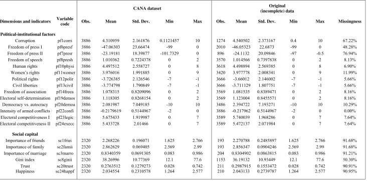
Political-institutional factors

Corruption pf1corri 3886 4.310959 2.161876 0.1121457 10 1274 4.540502 2.373167 0.4 10 67.22% Freedom of press I pf6presf 3886 -47.06303 23.66474 -99 0 2010 -46.05323 22.6873 -99 0 48.28% Freedom of press II pf7presr 3886 -23.19181 18.39877 -101.7329 0 896 -24.1132 20.09846 -97 -0.5 76.94% Freedom of speech pf8presh 3886 1.010362 0.7224378 0 2 3570 1.014566 0.7397838 0 2 8.13% Human rights pf10physi 3886 4.497512 2.558727 0 8 3618 4.498894 2.569385 0 8 6.90% Women’s rights pf11womer 3886 3.976016 1.991885 0 9 3420 3.977778 2.008341 0 9 11.99% Political rights pf12polir 3886 -3.726385 2.126546 -7 -1 3666 -3.66012 2.146002 -7 -1 5.66%

Civil liberties pf13civil 3886 -3.774798 1.790849 -7 -1 3666 -3.711129 1.807751 -7 -1 5.66% Freedom of association pf14freea 3886 1.078315 0.8209096 0 2 3569 1.081535 0.8389471 0 2 8.16% Electoral self-determination pf19demos 3886 1.118305 0.8268154 0 2 3569 1.123004 0.8455571 0 2 8.16% Democracy vs. autocracy pf20demoa 3886 2.081987 7.049185 -10 10 3486 2.394722 7.193271 -10 10 10.29% Intensity of armed conflicts pf22confi 3886 -0.2179619 0.5144967 -2 0 3886 -0.217962 0.5144967 -2 0 0.00% Electoral competitiveness I pf23legic 3886 5.675433 1.919987 0 7 3589 5.740039 1.968286 0 7 7.64% Electoral competitiveness II pf24execc 3886 5.433728 2.01466 0 7 3589 5.472137 2.071984 0 7 7.64%

Social capital

Importance of friends sc1friei 2320 2.268226 0.196071 1.625 2.766 193 2.270788 0.2485897 1.625 2.766 91.68% Importance of family sc2famii 2320 2.862629 0.069405 2.569 2.99 193 2.856347 0.0904246 2.569 2.99 91.68% Importance of marriage sc3marro 2320 0.8340359 0.0691305 0.083 0.986 204 0.8304902 0.0863815 0.083 0.986 91.21%

[image:25.842.59.791.100.461.2]

(26)

[image:26.842.563.825.143.299.2]

Figure 2: Innovation and technological capabilities (1980 – 2008) - 0 50 0 0 0 10 00 00 15 00 00 20 00 00 De ns it y

0 .00005 .0001 .00015 .0002 .00025

di6patecap

1980 2008

kernel = epanechnikov, bandwidth = 8.289e-07

Innovation - USPTO Granted Patents

0 .5 1 1. 5 De ns it y

-1 0 1 2 3

dicomposite

1980 2008

kernel = epanechnikov, bandwidth = 0.1059

Innovation and Technological Capabilities

0 .2 .4 .6 .8 1 De ns it y

0 1 2 3 4 5

di16merdt

1980 2008

Innovation and Technological Capabilities (94 Countries) - GERD % GDP

Japan

South Korea

United Kingdom United States

-0.5 0 0.5 1 1.5 2 2.5 3 3.5 198 0 198 1 198 2 198 3 198 4 198 5 198 6 198 7 198 8 198 9 199 0 199 1 199 2 199 3 199 4 199 5 199 6 199 7 199 8 199 9 200 0 200 1 200 2 200 3 200 4 200 5 200 6 200 7 200 8

Innovation and Technological Capabilities -Composite Indicator (1980 - 2008)

Brazil China India Japan South Korea United Kingdom United States

Japan South Korea United Kingdom United States 0 0.00005 0.0001 0.00015 0.0002 0.00025 0.0003 0.00035 198 0 198 1 198 2 198 3 198 4 198 5 198 6 198 7 198 8 198 9 199 0 199 1 199 2 199 3 199 4 199 5 199 6 199 7 199 8 199 9 200 0 200 1 200 2 200 3 200 4 200 5 200 6 200 7 200 8 P a tent s G ra n ted per m illi on peopl e

Innovation and Tech ogical Capabilities -USPTO Patents Granted (1980 - 2008)

nol Brazil China India Japan South Korea United Kingdom United States 0 0.5 1 1.5 2 2.5 3 3.5 198 0 198 1 198 2 198 3 198 4 198 5 198 6 198 7 198 8 198 9 199 0 199 1 199 2 199 3 199 4 199 5 199 6 199 7 199 8 199 9 200 0 200 1 200 2 200 3 200 4 200 5 200 6 200 7 200 8 % o f G D P

Innovation and Technological Capabilities -GERD as % of GDP (1980 - 2008)

(27)

[image:27.842.24.832.109.492.2]

Figure 3: Education system and human capital (1980 – 2008) Brazil China India Russia South Korea United States -1 -0.5 0 0.5 1 1.5 1 980 1 981 1 982 1 983 1 984 1 985 1 986 1 987 1 988 1 989 1 990 1 991 1 992 1 993 1 994 1 995 1 996 1 997 1 998 1 999 2 000 2 001 2 002 2 003 2 004 2 005 2 006 2 007 2 008

Education System and Human Capital -Composite Indicator (1980 - 2008)

Brazil China India Russia South Korea United States

Brazil China India Russia South Korea United States 0 2 4 6 8 10 12 14 1 980 1 981 1 982 1 983 1 984 1 985 1 986 1 987 1 988 1 989 1 990 1 991 1 992 1 993 1 994 1 995 1 996 1 997 1 998 1 999 2 000 2 001 2 002 2 003 2 004 2 005 2 006 2 007 2 008 M e an Y ears o f S c h o o li n g

Education System and Human Capital -Mean Years of Schooling (1980 - 2008)

Brazil China India Russia South Korea United States

Brazil China _India Russia United States 20 40 60 80 100 120 1 980 1 981 1 982 1 983 1 984 1 985 1 986 1 987 1 988 1 989 1 990 1 991 1 992 1 993 1 994 1 995 1 996 1 997 1 998 1 999 2 000 2 001 2 002 2 003 2 004 2 005 2 006 2 007 2 008 R a ti o o f to ta l e n ro ll m e n t

Education System and Human Capital -Secondary Enrollment (1980 - 2008)

Brazil 0 .0 5 .1 .1 5 De ns it y

0 5 10 15

es10schom

1980 2008

Education System - Mean years of schooling

0 .0 0 5 .0 1 .0 1 5 De n s it y

0 50 100 150 200

es2enros

1980 2008

Education System - Secondary Enrollment

0 .2 .4 .6 De n s it y

-2 -1 0 1 2

escomposite

1980 2008

Education System - Composite Indicator

(28)

[image:28.842.29.830.106.474.2]

Figure 4: Infrastructures (1980 – 2008) 0 .0 0 2 .0 04 .0 06 .00 8 De n s it y

0 500 1000 1500 2000 2500

i6telecap

1980 2008

Infrastructure - Telephony Penetration

0 .0 0 0 1 .0 00 2 .0 0 0 3 De ns ity

0 10000 20000 30000 40000

i4elecc

1980 2008

Infrastructure - Electricity Consumption

0 .2 .4 .6 .8 De n s it y

-1 0 1 2 3

icomposite

1980 2008

Infrastructure - Composite Indicator

Brazil

China India

Japan

Russia South Korea

United States 0 3000 6000 9000 12000 15000 1 980 1 981 1 982 1 983 1 984 1 985 1 986 1 987 1 988 1 989 1 990 1 991 1 992 1 993 1 994 1 995 1 996 1 997 1 998 1 999 2 000 2 001 2 002 2 003 2 004 2 005 2 006 2 007 2 008 kW h p e r ca p it a

Infrastructures - Electricity Consumption (1980-2008)

Brazil China India Japan Russia South Korea United States -1 -0.5 0 0.5 1 1.5 2 1 980 1 981 1 982 1 983 1 984 1 985 1 986 1 987 1 988 1 989 1 990 1 991 1 992 1 993 1 994 1 995 1 996 1 997 1 998 1 999 2 000 2 001 2 002 2 003 2 004 2 005 2 006 2 007 2 008

Infrastructures - Composite Indicator (1980-2008)

Brazil China India Japan Russia South Korea United States

Brazil China India Japan Russia South Korea United States 0 400 800 1200 1600 1 980 1 981 1 982 1 983 1 984 1 985 1 986 1 987 1 988 1 989 1 990 1 991 1 992 1 993 1 994 1 995 1 996 1 997 1 998 1 999 2 000 2 001 2 002 2 003 2 004 2 005 2 006 2 007 2 008 T e le p h o n e su scri b ers p e r 1 000 p e o p le

Infrastructures - Telephony penetration (1980-2008)

(29)

[image:29.842.21.842.102.474.2]

Figure 5: Economic competitiveness (1980 – 2008) Brazil China Russia South Korea United Kingdom United States -1 0 1 2 1 980 1 981 1 982 1 983 1 984 1 985 1 986 1 987 1 988 1 989 1 990 1 991 1 992 1 993 1 994 1 995 1 996 1 997 1 998 1 999 2 000 2 001 2 002 2 003 2 004 2 005 2 006 2 007 2 008

Economic Competitiveness - Composite Indicator (1980 - 2008)

Brazil China Russia South Korea United Kingdom United States

Brazil China Russia South Korea United Kingdom United States -750 -650 -550 -450 -350 -250 -150 19 80 19 81 19 82 19 83 19 84 19 85 19 86 19 87 19 88 19 89 19 90 19 91 19 92 19 93 19 94 19 95 19 96 19 97 19 98 19 99 20 00 20 01 20 02 20 03 20 04 20 05 20 06 20 07 20 08 T im e ( d ays)

Economic Competitiviness - Enforcing Contracts (Time) (1980 - 2008)

Brazil China Russia South Korea United Kingdom United States -10 40 90 140 190 240 1 980 1 981 1 982 1 983 1 984 1 985 1 986 1 987 1 988 1 989 1 990 1 991 1 992 1 993 1 994 1 995 1 996 1 997 1 998 1 999 2 000 2 001 2 002 2 003 2 004 2 005 2 006 2 007 2 008 % G D P

Economic Competitiviness - Banking Credit as % of GDP (1980 - 2008)

0 .0 00 5 .0 0 1 .0 01 5 .0 0 2 De ns it y

-1500 -1000 -500 0

ec8contt 1980 2008

Economic Competitiveness - Enforcing Contracts (Time)

0 .0 0 5 .0 1 .0 15 De ns it y

-100 0 100 200 300

ec14credg 1980 2008

Economic Competitiveness - Banking Credit as % of GDP

0 .2 .4 .6 .8 De ns it y

-2 -1 0 1 2

eccomposite 1980 2008

(30)

[image:30.842.32.823.113.484.2]

Figure 6: Social capital (1980 – 2008) 0 .2 .4 .6 .8 De ns it y

-1.5 -1 -.5 0 .5 1

sc6composite 1980 2008

Social Capital (80 Countries) - Composite Indicator

0 1 2 3 4 De ns it y

0 .2 .4 .6 .8

sc20trust 1980 2008

Social Capital (80 Countries) - Trust

0 .5 1 1. 5 De n s it y

1.4 1.6 1.8 2 2.2 2.4

sc24happf 1980 2008

Social Capital (80 Countries) - Happiness Brazil China India Japan Russia United States -1.5 -1 -0.5 0 0.5 1 1.5 1 980 1 981 1 982 1 983 1 984 1 985 1 986 1 987 1 988 1 989 1 990 1 991 1 992 1 993 1 994 1 995 1 996 1 997 1 998 1 999 2 000 2 001 2 002 2 003 2 004 2 005 2 006 2 007 2 008

Social Capital - Composite Indicator (1980 - 2008)

Brazil China India Japan Russia United States

Brazil China India Japan Russia United States 0 0.1 0.2 0.3 0.4 0.5 0.6 0.7 1 980 1 981 1 982 1 983 1 984 1 985 1 986 1 987 1 988 1 989 1 990 1 991 1 992 1 993 1 994 1 995 1 996 1 997 1 998 1 999 2 000 2 001 2 002 2 003 2 004 2 005 2 006 2 007 2 008 % An sw ers M o st p e o p le ca n b e t ru s te d

Social Capital - Trust (1980 - 2008)

Brazil China India Japan Russia United States 1.4 1.6 1.8 2 2.2 2.4 1 980 1 981 1 982 1 983 1 984 1 985 1 986 1 987 1 988 1 989 1 990 1 991 1 992 1 993 1 994 1 995 1 996 1 997 1 998 1 999 2 000 2 001 2 002 2 003 2 004 2 005 2 006 2 007 2 008 L e vel o f h o m o se xu al it y j u st if icat io n

Social Capital - Happiness (1980 - 2008)

(31)

[image:31.842.36.839.118.481.2]

Figure 7: Political-institutional factors (1980 – 2008) Brazil China India Russia United States -1.6 -1.1 -0.6 -0.1 0.4 0.9 1.4 1 980 1 981 1 982 1 983 1 984 1 985 1 986 1 987 1 988 1 989 1 990 1 991 1 992 1 993 1 994 1 995 1 996 1 997 1 998 1 999 2 000 2 001 2 002 2 003 2 004 2 005 2 006 2 007 2 008

Political and Institutional System - Composite Indicator (1980 - 2008)

Brazil China India Russia United States

Brazil China India Russia United States 1 2 3 4 5 6 7 8 1 980 1 981 1 982 1 983 1 984 1 985 1 986 1 987 1 988 1 989 1 990 1 991 1 992 1 993 1 994 1 995 1 996 1 997 1 998 1 999 2 000 2 001 2 002 2 003 2 004 2 005 2 006 2 007 2 008 C or ru pt ion Fr e e Le v e l

Political and Institutional System - Corruption (1980 - 2008)

Brazil China India Russia Unites States -110 -90 -70 -50 -30 -10 1 980 1 981 1 982 1 983 1 984 1 985 1 986 1 987 1 988 1 989 1 990 1 991 1 992 1 993 1 994 1 995 1 996 1 997 1 998 1 999 2 000 2 001 2 002 2 003 2 004 2 005 2 006 2 007 2 008 L evel o f g o vern m en ta l c e n s o rsh ip