Adv. Radio Sci., 5, 367–372, 2007 www.adv-radio-sci.net/5/367/2007/ © Author(s) 2007. This work is licensed under a Creative Commons License.
Advances in
Radio Science
Analysis of the impact of map-matching on the accuracy of
propagation models
M. Neuland and T. Kürner
Institute of Communications Technology, Braunschweig Technical University, Germany
Abstract. Propagation models are very important for the
de-velopment and deployment of wireless communication net-works. They are able to predict the path loss for different propagation conditions, but cannot include all propagation phenomena in detail. This fact leads to variations between predicted and measured field strengths. These variations can be reduced by calibrating some parameters of the propaga-tion models with the help of exact measurement data. How-ever, two problems occur when applying measurement data. On the one hand, the maps used for the prediction have only a limited resolution. On the other hand, the GPS data are erroneous due to the limited GPS accuracy and due to sam-pling errors. These errors can lead to variations up to 200 m between the measured positions and the possible positions on the road network. Therefore, a map-matching algorithm has to be applied which projects the wrong GPS positions automatically onto the street vectors used for the predictions. Thus, a good basis of data for calibration can be created.
1 Introduction
Propagation models are a key element for the planning and deployment of wireless networks. With the help of these models coverage and capacity planning can be made and new site locations and system technologies can be tested easily and cost-efficiently. However, propagation models cannot include all propagation phenomena. The influence of sin-gle buildings, for example, cannot be considered if building data is not available for the prediction area. Furthermore, the propagation models provide only a simplified represen-tation of the propagation phenomena, i.e. Maxwell’s equa-tions are not solved exactly. And finally, propagation mod-els can only be as good as the input data as coordinates, an-Correspondence to: M. Neuland
tenna parameters etc. These three reasons are responsible for the inaccuracy of propagation models which leads to varia-tions between predicted and measured field strengths. These variations can be reduced by calibrating some parameters of the propagation models with the help of exact measurement data. However, two problems occur, when applying mea-surement data. On the one hand, the maps used for the pre-diction have only a limited resolution. The used maps have often become obsolete. On the other hand, the GPS data are erroneous due to the limited GPS accuracy and due to sam-pling errors. These errors can lead to variations up to 200 m between the recorded GPS position and the correct position on the road network (Pfoser and Jensen, 1999). The inac-curacy of the maps cannot be resolved, but the errors of the GPS can be reduced by applying a map-matching algorithm. Map-matching projects the wrong GPS positions automati-cally onto the street vectors used for the prediction. Thus, the wrong GPS positions can be corrected in a way so that an accurate analysis of propagation models is possible and a good basis of measurement data can be created for cali-bration which has an impact on the accuracy of propagation models.
The performance of the GPS data is described in Sect. 2. In Sect. 3, the map-matching algorithm is introduced, and finally, in Sect. 4, the influence of map-matching on the ac-curacy of propagation models is analysed with the help of CW measurements for 900 MHz.
2 GPS error
4.1356
4.1357
4.1357
4.1357
4.1358
4.1358
4.1359
4.136
4.136
4.1361
x 10
65.6889
5.689
5.6891
5.6892
5.6893
Fig. 1. Example for the measurement error of a measurement route
in Düsseldorf.
1 2 3
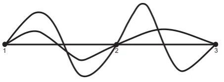
Fig. 2. Possible trajectories between three consecutive GPS
posi-tions.
is introduced in Sect. 2.2 as they are reported by Brakatsoulas et al. (2005) and Pfoser and Jensen (1999). The GPS errors are mostly determined by the time-varying constellation of the satellites and the built-up in the close vicinity of the GPS receiver (Modsching et al., 2006).
2.1 Measurement error
The measurement error due to the limited accuracy of the GPS causes the measured GPS positions not lying on the corresponding road network represented by street vectors, as shown in Fig. 1. The accuracy of the GPS can be described by two error distributions. The error in each of the three di-mensions and the error in time are assumed to be Gaussian and the error in the x-, y-plane is circular.
2.2 Sampling error
GPS records positions with a certain sampling rate. The driven route between these two consecutive positions can only be interpolated. An example for possible trajectories between three consecutive GPS positions is shown in Fig. 2. The interpolation is mostly done linearly which leads to inac-curacies. These inaccuracies increase with a decreasing sam-pling rate. Due to the samsam-pling error, the interpolated route between two consecutive GPS positions cannot be matched easily to edges of the road network. However, the possi-ble trajectory between two consecutively recorded positions
Fig. 3. Example for measured erroneous GPS positions.
is overall bounded by an error ellipse. This error ellipse depends on the sampling rate with which the positions are recorded and the velocity with which the GPS receiver is moved.
3 Map-matching
Map-matching is an algorithm which matches the measured erroneous GPS positions on the road network. For this, the road network has to be represented by street vectors. With the help of map-matching the GPS errors can be reduced. An example for measured erroneous GPS positions is shown in Fig. 3.
The developed algorithm consists of two parts. Firstly, a block-matching is applied which is described in Sect. 3.1, followed by an algorithm which projects the positions on the road network. This part of the map-matching algorithm is explained in Sect. 3.2.
3.1 Block-matching
Block-matching is an algorithm which is used for motion es-timation in video coding applications (Strutz, 2000). In case of map-matching the driven route is divided in partial routes with a certain number of measurement bins. These partial routes are moved with different increments along the x- and y-axis and diagonally to both axis. As a quality factor the sum of the distances of each position to the nearest street vector is used. The distance from a pointQto a street vector
ABis defined as in Eq. (1),
d =
(
de(Q, Q0) ifQ0∈[AB]
min(de(Q, A), de(Q, B)) elsewhere
(1)
whereQ0 is the orthogonal projection of Qon AB andde
M. Neuland and T. Kürner: Analysis of the impact of map-matching on the accuracy of propagation models 369
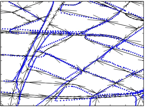
Fig. 4. Result of the block-matching algorithm for the route shown
in Fig. 3.
The applied algorithm uses block-matching twice. Firstly, a “rough” block-matching with relatively large increments and partial routes with many measurement bins is done in order to be able to overcome large variations. In the vicin-ity of the result of the first matching, another block-matching with smaller increments and smaller partial routes is used for fine tuning. In order to adapt the algorithm to dif-ferent situations, the number of measured points in the partial routes can be varied.
In some cases the measured GPS route is not only dis-placed, but also distorted. Thus, block-matching alone can-not match the whole route on the road network as can be seen in Fig. 4. The next step, the projection of the GPS positions on the street vectors, is also required. However, with the help of block-matching the probability is increased to match the positions on the correct street vectors.
3.2 Projection on the street vectors
The projection on the street vectors is similar to the algo-rithm introduced by Brakatsoulas et al. (2005). A position-by-position and edge-by-edge strategy is used. Starting from a correctly projected GPS position the candidates of street vectors for the next projection are determined. This set of street vectors includes the “neighbour” street vectors of the last matched street vector as well as the last matched street vector itself. As a quality factor the distance to the possible street vector as well as the orientation of the measurement route compared to the orientation of the street vectors are considered. The distance is calculated as in Eq. (1). The orientation is determined as the median of the orientations between the current point and the following two points. Big-ger differences between the orientation of the measurement route and the orientation of the street vectors are weighted more than smaller differences. An example for the result
af-Fig. 5. Result after projecting the positions on the road network for
the route shown in Fig. 3.
ter projecting the positions on the road network is shown in Fig. 5.
For this part of the map-matching algorithm a correct start-ing point is very important. If the first point of the measure-ment route is projected onto the wrong street vector, the fol-lowing points are also projected wrongly. Thus, the initiali-sation plays a decisive role. For initialiinitiali-sation, all street vec-tors in an area of 120 m around the first point are considered. The street vector with the smallest distance and an orienta-tion comparable to the orientaorienta-tion of the measurement route at the first point is chosen as the street vector on which the first point is projected. If the distance between two consecu-tive projection points becomes much larger than the distance between the corresponding points of the measurement route or if the distance between the GPS position and the matched position exceeds a certain threshold then a new initialisation is made.
3.3 Postprocessing
In some areas, especially in dense urban areas, the recorded GPS signal is so erroneous that even a manual matching is hardly possible. These parts of the measurement route which are so much distorted cannot be matched correctly by the map-matching algorithm. In order to be able to make pre-cise analyses of the propagation model and to create a good basis of measurement data for calibration these parts of the measurement route have to be removed manually by a visual inspection.
4 Analysis of the accuracy of propagation models
Fig. 6. Measurement route in Düsseldorf with 20 815 bins after
map-matching.
Table 1. Mean error and standard deviation for the example in
Fig. 8.
number of bins mean error standard deviation
original route 85 7.3 4.9
matched route 160 −1.3 4.4
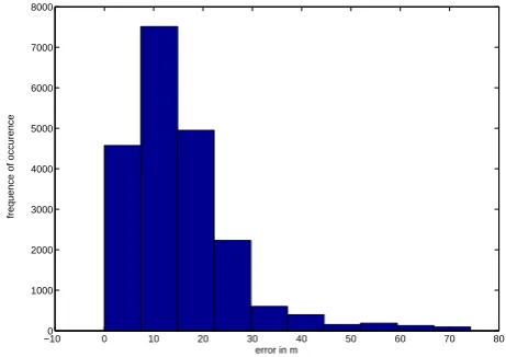
used. For a detailed analysis one site in Düsseldorf with 20 815 measurement bins is picked. The map-matching al-gorithm described in Sect. 3 is applied which leads to the result shown in Fig. 6 for the chosen site in Düsseldorf. The “error” distribution between the original and the matched po-sitions for this measurement route is shown in Fig. 7. It can be seen that the original and the matched positions mostly differ about 10 m, but that divergences up to 75 m also occur. For the analysis, measured values smaller than−110 dBm are discarded because the receiver sensitivity is−110 dBm. The analysed propagation model is introduced in Sect. 4.1. The results of the analysis with the original and the matched measurement data are described in Sects. 4.2 and 4.3. 4.1 Propagation model
For the prediction the propagation model described by Kürner and Meier (2002) is used. It consists of three sub models. Basis of this propagation model is the vertical plane model (VPM). It is used to determine the path loss in a street canyon in case of line-of-sight and the path loss over rooftops in case of non-line-of-sight, respectively. This model uses raster data with a resolution of 5 m. In an area about 500 m around the base station single scattering processes are con-sidered additionally by the multipath model (MPM). In order to determine possible scattering areas, vector data with a very high resolution is used. If there is vegetation between the
Fig. 7. Divergence between the original and the matched
measure-ment route in Düsseldorf in m.
base station and the mobile station, a vegetation attenuation (VegMod) is calculated in addition to the VPM and MPM. 4.2 Analysis results for a site in Düsseldorf
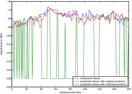
The results of the propagation model are analysed with the original and the matched measurement route. The predicted signal levels for both routes compared to the measured signal levels are plotted in Fig. 8 for 160 bins of the measurement route in Düsseldorf. It can be seen that the predicted values to which map-matching has been applied (red curve) fit the measured values (blue curve) quite good although no cali-bration has been applied. In contrast, the predicted values which have not been matched (green curve) show larger dif-ferences. Furthermore, the predicted bins marked with a de-fault value of−150 dBm have to be discarded because these pixels represent indoor positions although the measured val-ues have been recorded outdoor. This leads to a data loss of about 50% for this part of the measurement route. The corre-sponding mean error1and standard deviation can be seen in Table 1. For the prediction with the matched measured po-sitions, both, the mean error and the standard deviation, are smaller than for the prediction with the originally measured positions. Especially the lower standard deviation for the prediction with the matched positions shows that the prop-agation phenomena are better modeled than for the positions which have not been matched.
The fact that the matched positions describe the measured values better than the not-matched positions can be seen in Table 2. For this analysis, all measured values which corre-spond to indoor positions are discarded from the whole origi-nal and matched measurement routes so that both routes have
1The error is calculated asP
pred−Pmeas, wherePpredis the
pre-dicted signal level in dBm andPmeasthe measured one. Therefore,
M. Neuland and T. Kürner: Analysis of the impact of map-matching on the accuracy of propagation models 371
0 20 40 60 80 100 120 140 160
−160 −150 −140 −130 −120 −110 −100 −90 −80 −70 −60
measurement bins
signal level in dBm
measured values
predicted values with original positions predicted values with matched positions
Fig. 8. Plot of the measured values as well as the predicted values
for the original and the matched measurement route, respectively.
the same bins. For this extract of data the standard deviation for the matched measurement route is also lower than the standard deviation of the original one.
4.3 Analysis results for nine sites in five large German cities
In order to get more information about the impact of map-matching on the accuracy of propagation models, CW mea-surements at 900 MHz for nine sites in Düsseldorf (sites 1 and 2), Frankfurt (site 3), Berlin (sites 4, 5, and 6), Leipzig (sites 7 and 8), and Munich (site 9) are analysed. The predic-tions with the original and matched measurement routes are compared to the measured values. Furthermore, this mea-surement data is used for calibrating the propagation model described in Sect. 4.1. The standard deviations for these sites are plotted in Fig. 9 for the original and the matched mea-surement route in comparison to the uncalibrated model as well as for the matched measurement route in comparison to the calibrated model. It can be seen that the applied map-matching algorithm can reduce the standard deviations for almost all sites. Only sites 7 and 8 have higher standard de-viations after map-matching. However, for sites 3, 4, and 5 the standard deviations can be reduced significantly. After calibration the standard deviations can be reduced even more. For most of the sites, the standard deviations are around 7 dB, for sites 2 and 9 they are even smaller than 6 dB. This shows that a good basis of measurement data for calibration has been found by applying a map-matching algorithm to the er-roneous GPS positions of the measurement data.
5 Conclusions
In this paper it is shown that measurement data recorded with GPS are erroneous due to the limited accuracy of GPS and due to sampling errors. These errors can lead to
varia-1 2 3 4 5 6 7 8 9
0 2 4 6 8 10 12 14
sites
standard deviation in dB
original matched calibrated
Fig. 9. Standard deviations for nine sites in five large German cities
before and after applying map-matching.
Table 2. Mean error and standard deviation for the measurement
route in Düsseldorf without indoor pixels.
mean error standard deviation
original measurement route 3.7 9.8
matched measurement route 4.1 9.6
tions up to 200 m between the recorded GPS positions and the road network. Thus, precise analysis and a good cali-bration of propagation models is hardly possible with this erroneous measurement data. However, the erroneous GPS positions can be corrected by applying a map-matching al-gorithm as introduced in Sect. 3. This alal-gorithm projects the GPS positions on the road network. Analysing the pre-dicted field strengths for the corrected measured positions leads to lower standard deviations in comparison to the pre-dicted field strengths for the erroneous measured positions as shown in Sect. 4. Especially the analysis in Sect. 4.3 shows the reduction of the standard deviations after map-matching. Using this matched measurement data for calibration reduces the standard deviation even more. Thus, a precise analysis is possible and a good basis of measurement data can be cre-ated if map-matching is applied to the erroneous measure-ment data recorded with GPS.