R E S E A R C H A R T I C L E
Open Access
An error estimator for real-time simulators
based on model order reduction
Icíar Alfaro
1†, David González
1†, Sergio Zlotnik
2†, Pedro Díez
2†, Elías Cueto
1*†and Francisco Chinesta
3†*Correspondence:
†Icíar Alfaro, David González,
Sergio Zlotnik, Pedro Díez, Elías Cueto and Francisco Chinesta contributed equally to this work. 1Aragon Institute of Engineering Research, Universidad de Zaragoza, María de Luna, s.n., 50018 Zaragoza, Spain Full list of author information is available at the end of the article
Abstract
Model order reduction is one of the most appealing choices for real-time simulation of non-linear solids. In this work a method is presented in which real time performance is achieved by means of the off-line solution of a (high dimensional) parametric problem that provides a sort of response surface orcomputational vademecum. This solution is then evaluated in real-time at feedback rates compatible with haptic devices, for instance (i.e., more than 1 kHz). This high dimensional problem can be solved without the limitations imposed by the curse of dimensionality by employing proper
generalized decomposition (PGD) methods. Essentially, PGD assumes a separated representation for the essential field of the problem. Here, an error estimator is proposed for this type of solutions that takes into account the non-linear character of the studied problems. This error estimator allows to compute the necessary number of modes employed to obtain an approximation to the solution within a prescribed error tolerance in a given quantity of interest.
Keywords: Error estimation, Real time, Model order reduction, Proper generalized decomposition
Background
Real-time simulation of non-linear solids is always a delicate task due to the heavy com-putational cost associated with the linearization of the equations. Applications are ubiq-uitous, ranging from industrial uses [1] to surgery planning and training [2,3] or movies [4].
Probably, the field in which more effort has been paid to the development of real-time simulation techniques is that of computational surgery [5–10]. This is because surgery training systems are equipped with haptic peripherals, those that provide the user with realistic touch sensations (force feedback). Just like some 25 pictures per second are necessary for a realistic perception of movement in films, haptic feedback needs for some 500 Hz to 1 kHz in order to achieve the necessary realism. The difficulty of the task is thus readily understood: to perform 500–1000 simulations of highly non-linear solids (soft tissues are frequently assumed to be hyperelastic), possibly suffering contact, cutting, etc. Among the very few truly non-linear surgery simulators developed so far, one can cite [10–13]. Essentially, the former employ some type of explicit, lumped mass, Lagrangian finite elements to perform the simulations, possibly including an intensive usage of GPUs.
©2015 Alfaro et al. This article is distributed under the terms of the Creative Commons Attribution 4.0 International License (http:// creativecommons.org/licenses/by/4.0/), which permits unrestricted use, distribution, and reproduction in any medium, provided you give appropriate credit to the original author(s) and the source, provide a link to the Creative Commons license, and indicate if changes were made.
However, in previous works of the authors, see [13–16], a different approach has been studied by employing model order reduction techniques, see Fig.1.
Basically, our approach to real-time simulations consists on the off-line computation of a sort of high-dimensional solution to the problem at hand,
u=u(x, t, q1, q2,. . ., qp), (1) whereurepresents the essential field of the problem (usually, the displacement field of the solid),xthe coordinates of each physical point, andq1, q2,. . ., qpa set of parameters that could affect the solution and whose meaning will be clear in brief.
Equation (1) thus represents a sort ofresponse surfacein the sense that it provides with the solution for any physical coordinate, time instant and value of thepparameters. Instead ofresponse surface, and to highlight the fact that no set ofa prioriexperiments will be necessary to obtain such a response in our method, we prefer to call Eq. (1) acomputational vademecum[17], inspired by the work of ancient engineers (such as Bernoulli, for instance [18]), who compiled sets of known solutions to problems of interest.
The problem with an approach such as that introduced in Eq. (1) is that such an expres-sion is inherently high dimenexpres-sional. If we try to discretize the governing equations of the problem so as to obtain an approximation to Eq. (1), and do it by a mesh-based method such as finite differences, volumes or elements, we will soon realize that the complexity of the problem will make us run out of computer memory very soon. This is due to the well-known exponential growth of the number of degrees of freedom (nodes of the mesh) with the number of dimensions of the problem. In other words, the well-knowncurse of dimensionality[19].
In order to overcome the curse of dimensionality, the authors proposed some years ago a technique inspired by proper orthogonal decomposition methods (POD) that generalizes its properties to high dimensional spaces and operatesa priori. Such a technique has been coined as proper generalized decomposition (PGD) [20–24] and its main characteristic is to assume that the essential field (1) can be approximated in a separated form, i.e.,
u(x, t, q1, q2,. . ., qp)≈ n
i=1
Fi(x)◦Gi(t)◦Q1i(q1)◦Q2i(q2)◦. . .◦Qpi(qp), (2)
where the symbol “◦” appears for the Hadamard, Schur or entry-wise product of vectorial functions. Since functionsFi(x),Gi(t),Q1i(q1),Q2i(q2),. . .,Qpi(qp) are a priori unknown,
one readily recognizes the inherent non-linear character of the problem of finding such an approximation (even if the governing equations are linear). PGD operates through a greedy algorithm, in which usually a fixed point alternating directions algorithm is used. More details will be given in the “Formulation of the problem in a PGD setting”.
One crucial problem related to such an approximation, see Eq. (2), is the choice of the number of termsnemployed in the approximation. Being the main objetive of a simulator to provide the user with a realistic force feedback, the aim of the work presented herein is to develop a suitable error estimator that allows us to fix the number of functional products
n necessary for a given tolerance in the error of the transmitted force. The literature on error estimation for model order reduction is vast, see [25–31], to name but a few. In “Formulation of the problem in a PGD setting” we recall the basics of the PGD approach to the problem at hand. In “One possible explicit linearization of the formulation” we revisit one of the possible linearization of the problem and, finally, in “An error estimator based on the dual formulation” we develop the sought error estimator for the force feedback. The paper is completed with two different numerical examples in “Numerical examples” that show the performance of the method.
Formulation of the problem in a PGD setting
As a model non-linear problem hyperelasticity has been chosen. This constitutes a suffi-ciently general theory, with important implications in the simulation of soft living tissues [32,33], for instance, and therefore in surgical simulators as an ubiquitous example of the restrictions placed by real-time constraints.
In what follows we follow closely the explicit linearization procedure first developed by the authors in [13], although more sophisticated approaches were developed in [15]. For the sake of simplicity, consider a particularly useful instance of the vademecum given by Eq. (1),
u=u(x,s),
i.e., a generalized solution of the displacement field of a solid undergoing a load at any possible point of its boundary,s. Therefore, the loading pointsacts here as the parameter
q1in (1). For simplicity, we assume the acting forcet as vertical and of unity module
(a more general setting can be established by letting t itself be an additional vectorial parameter). Under this rationale, the weak form of the static equilibrium equations of the solid can be established asfind the displacementu∈H1such that for allu∗∈H1
0:
¯
∇
(s)u∗:σdd¯ =
¯
t2
u∗·tdd¯ (3)
where=u∪trepresents the boundary of the solid, divided into essential and natural regions, and wheret=t1∪t2, i.e., regions of homogeneous and non-homogeneous,
respectively, natural boundary conditions.∇(s)stands for the symmetric part of the gradi-ent. ¯ ⊆t2represents the possible loading area within the exposed surface of the body
of the organ surface accesible for the surgeon. Here,t =ek·δ(x−s), whereδrepresents the Dirac-delta function andekthe unit vector along thez-coordinate axis.
In the spirit of PGD techniques, the external load is then decomposed (by applying SVD techniques, for instance) as
tj≈ m
i=1
fji(x)gji(s)
where mrepresents the order of truncation andfi
j, gji represent thejth component of vectorial functions in space and boundary position, respectively. Following Eq. (2), the high dimensional solution of the problem will be sought as
unj(x,s)=
n
k=1
Xjk(x)·Yjk(s), (4) where the termujrefers to thej-th component of the displacement vector,j=1,2,3 and functionsXkandYkrepresent the separated functions used to approximate the unknown field.
PGD techniques proceed by finding iteratively new terms improving this approximation in a greedy framework. Therefore, if a new functional pairR(x)◦S(s) is sought,
unj+1(x,s)=ujn(x,s)+Rj(x)·Sj(s), (5) a linearization algorithm is compulsory, since the unknown is now a pair of functions. This is usually accomplished by iterative fixed point, alternating directions algorithms that proceed as follows.
Computation ofS(s) assumingR(x) is known
If standard assumptions of variational calculus are applied,
u∗j(x,s)=Rj(x)·Sj∗(s). (6) This admissible variation of the (high dimensional) displacement field, indicated by the star symbol, is then injected into the weak form of the problem, Eq. (3), thus giving
¯
∇
(s)(R◦S∗) :C:∇(s)
n
k=1
Xk◦Yk+R◦S
dd¯
= ¯ t2
(R◦S∗)·
m
k=1
fk◦gk
dd¯, (7) or, ¯ ∇
(s)(R◦S∗) :C:∇(s)(R◦S)dd¯
= ¯ t2
(R◦S∗)·
m
k=1
fk◦gk
dd¯−
¯
∇
(s)R◦S∗·Rndd¯, (8) whereRnrepresents:
Rn=C:∇(s)un. (9)
Since the symmetric gradient operates on spatial variables only, we arrive at:
¯
(∇
(s)R◦S∗) :C: (∇(s)R◦S)dd¯
= ¯ t2
(R◦S∗)·
m
k=1
fk◦gk
dd¯−
¯
where all the terms depending onx are known and hence all integrals over andt2
(support of the regularization of the initially punctual load) can be computed to arrive at an equation forS(s).
Computation ofR(x) assumingS(s) is known
Proceeding in an entirely similar way,
u∗j(x,s)=R∗j(x)·Sj(s), (11) which, substituted in the weak form of the problem, Eq. (3), gives
¯
∇
(s)(R∗◦S) :C:∇(s)
n
k=1
Xk◦Yk+R◦S
dd¯
=
¯
t2
(R∗◦S)·
m
k=1
fk◦gk
dd¯. (12) Again, all the terms depending ons(load position) can be integrated on ¯, thus giving an elasticity-like problem to obtain the functionR(x).
One possible explicit linearization of the formulation
The simplest hyperelastic constitutive model is the Kirchhoff–Saint Venant (KSV) model. Despite its well-known instabilities in compression, KSV provides with a very neat for-mulation in which to apply the developments that are to come. Therefore, for the sake of simplicity, we assume that the energy density functional is given by
= λ
2(tr(E))
2+μE:E (13)
whereλandμare Lame’s constants. The Green-Lagrange strain tensor,E, is classically defined as
E= 1 2(F
TF−I)=∇(s)u+ 1
2(∇u·∇u
T) (14)
whereF = ∇u+Iis the gradient of deformation tensor. Correspondingly, the second Piola-Kirchhoff stress tensor can be obtained by
S= ∂∂E(E) =C:E (15)
in whichCis the fourth-order constitutive (here, linear elastic) tensor.
The simplest linearization of the resulting problem comes from an explicit assumption in which load is applied in a series of pseudo-time incrementst, producing displacement incrementsu(x,s). At each time increment, the previously described PGD fixed point
alternating directions algorithm is employed. So, by introducing the non-linear strain measure given by Eq. (14), into this incremental framework, the following expression is obtained:
Et+t=∇ s
ut+u+ 1 2
∇(ut+u)·∇T(ut+u) . (16) Equivalently, admissible variations of strain take the form
E∗=∇(s)(u∗)+ 1
2(∇(u
∗))·∇T(ut+u)+ 1
2∇(u
t+u)·∇T(u∗)
¯
(t)
E∗:C:Edd¯
=
¯
(t)
∇(s)(u∗)+∇(u∗)·∇T(ut+u) :C
:
∇s
ut+u+1 2
∇(ut+u)·∇T(ut+u) dd¯. (18) To linearize Eq. (18), in [13] a strategy is proposed by keeping in the formulation only constant terms and those linear in u. The resulting weak form is composed by the following long albeit simple collection of terms:
¯
(t)
E∗:C:Edd¯
=
¯
(t)∇
(s)(u∗) :C:∇(s)utdd¯ +
¯
(t)∇
(s)(u∗) :C:∇(s)(u)dd¯ +
¯
(t)∇
(s)(u∗) :C: 1
2∇u
t·∇Tutdd¯ +
¯
(t)∇
(s)(u∗) :C:∇ut·∇T(u)dd¯ +
¯
(t)∇
(u∗)·∇Tut:C:∇(s)utdd¯
+
¯
(t)∇
(u∗)·∇Tut:C:∇(s)(u)dd¯
+
¯
(t)∇
(u∗)·∇Tut:C: 1 2∇u
t·∇Tutdd¯ +
¯
(t)∇
(u∗)·∇Tut:C:∇ut·∇T(u)dd¯
+
¯
(t)∇
(u∗)·∇T(u) :C:∇(s)utdd¯
+
¯
(t)∇
(u∗)·∇T(u) :C: 1 2∇u
t·∇Tutdd¯. (19)
Despite the apparent complexity of these equations, a very simple scheme results that has provided, however, very good results.
However, a critical issue remains in this case (or, in general, when dealing with PGD approximations of non-linear problems), which is that of selecting the number of termsn
composing the approximation, see Eq. (4). This must be done on the basis of predictions given by a suitable error estimator, which is the main objective of this work and will be detailed in the following section.
An error estimator based on the dual formulation
What Eq. (19) represents in fact is an incremental, explicit linearization of the originally non-linear problem. Thus, by using a compact notation, we can say that at pseudo-time steppthe weak form of the problem looks like
Errors in the PGD solution of this linearized equation come from two sources. First, the separated representation of the solution, given by Eq. (2), involves a truncation of the sum at a numbernof terms. Secondly, the sought functionsFi,Gi, ..., are actually expressed by projecting them onto a finite element mesh of sizeh. In brief, the following diagram depicts the situation:
un
h(x,s) unh=∞(x,s) =uh
un
h=0(x,s) u(x,s)
ePGD
eFEM eFEM
ePGD e
where we have denotedePGD= unh=∞−unh = u−uhn=0andeFEM= unh=0−unh = u−uh. Finally, the sought, total committed error would bee= u−unh.
It is noteworthy to mention that, if the FE mesh size,his not chosen judiciously, the total error in the simulation, composed by the sum of the FEM error plus the PGD error, will never get below a prescribed tolerance despite the number of modes added to the PGD approximation. Therefore, care must be paid not only to the number of termsnin the PGD approximation, but to the mesh size,h.
The objective of this paper is to determine the number of terms necessary to reach some error threshold in the non-linear problem given by Eq. (3), equipped with the non-linear constitutive equations (13). This error assessment is performed by establishing a (here, linear) functional o(·), used to extract certain quantity of interest. For the application we are pursuing (surgery simulators with haptic feedback), this quantity of interest would be the perceived reaction force at the peripheral. The main advantage of the linearization introduced in Eq. (19) is precisely that within each time step the increment in the reaction force is a linear function of the increment of (vertical, for simplicity) displacement (at the loading point), i.e.,
o(un
h)=uz(x0,s0),
in other words, the increment of vertical displacement atx0provoked by the load acting
ats0. In our approach, since we interested in estimating the error on the force value, we
simply takex0=s0, withx0a particular point on the loading surface.
Following [34] (although other approaches are equally feasible for PGD, see [35–37]), the error in the quantity of interest is obtained through an auxiliary problem, often referred to as dual or adjoint problem. In [34], the exact solution of the auxiliary problem is replaced by a more accurate solution, which in a PGD context can naturally be obtained by performing some extra enrichment increments (i.e., lettingngrow sufficiently to a valueN).
Therefore, the dual or adjoint problem will now look like
a(u∗,ϕ)= o(u∗), (20) withϕthe dual unknown. The error in the quantity of interest could therefore be computed by
o(e)=b(ϕ)−a(un h,ϕ), or, equivalently,
X Y Z
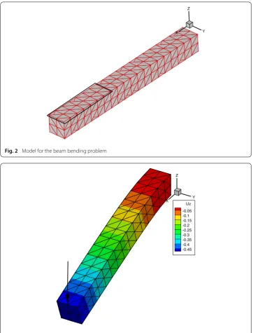
Fig. 2 Model for the beam bending problem
X Y Z
Uz -0.05 -0.1 -0.15 -0.2 -0.25 -0.3 -0.35 -0.4 -0.45
Fig. 3 Deformed beam for a particular location of the point load
withε= ϕ−ϕh. As mentioned before, the exact solution of the dual problem,ϕis not often available, so that it is approximated as
ϕ≈ϕNn h .
Although different possibilities exist, see for instance [31], in [34] different strategies were analyzed to determine the necessary value ofN. For instance, results takingN =n+5,
N =2nor, simply,N =nwere analyzed. In general some extra terms, say 5, are enough to determine a good dual solution.
1.5
1
0.5
0 0 0.1 0.2
0.1
0 0.2
a
1.5
1
0.5
0 0 0.1 0.2
0.1
0 0.2
b
1.5
1
0.5
0 0 0.1 0.2
0.1
0 0.2
c
1.5
1
0.5
0 0 0.1 0.2
0.1
0 0.2
d
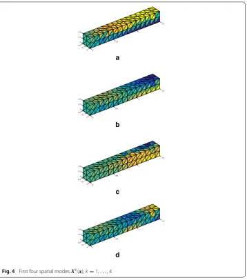
Fig. 4 First four spatial modesXk(x),k=1,. . .,4
Numerical examples Cantilever beam
We consider the example of a cantilevered Kirchhoff-Saint Venant beam whose geometry is shown in Fig.2. Beam nodes are assumed fixed at one of the ends, while the rest of the degrees of freedom are assumed to be free. The mesh is composed by tetrahedral elements, with 3×3 nodes in the 40×40 mm2 cross-section and 21 nodes in the longitudinal direction, 400 mm long. Material parameters were Young’s modulusE=2×10¹¹Pa and Poisson’s coefficientν = 0.3. The applied force is assumed to be always vertical and its value taken as 108N.
The deformed configuration of the beam for one particular location of the load is shown in Fig.3. The four first modesXk(x),k=1,2,. . .,4 are shown in Fig.4.
0.15 0.2 0.25 0.8 0.9 1 1.1 1.2 1.3 1.4 1.5 0 0.05 0.1 0.15 0.2 a 0.15 0.2 0.25 0.8 0.9 1 1.1 1.2 1.3 1.4 1.5 0 0.05 0.1 0.15 0.2 b 0.15 0.2 0.25 0.8 0.9 1 1.1 1.2 1.3 1.4 1.5 0 0.05 0.1 0.15 0.2 c 0.15 0.2 0.25 0.8 0.9 1 1.1 1.2 1.3 1.4 1.5 0 0.05 0.1 0.15 0.2 d
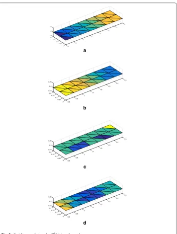
Fig. 5 First four spatial modesYk(s),k=1,. . .,4
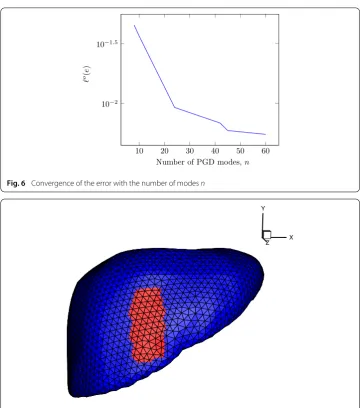
The loading process was solved by takingp=8 pseudo-time steps, both for the primal and dual problems. The dual problem was solved by applying a stopping criterion such thatϕn+1−ϕn ≤ 10−8. With such a criterion, the computation ofϕinvolved eight
modes, one per time step. The evolution of the predicted error with the number of modes
nemployed in the computation of the primal variable is shown in Fig.6.
10 20 30 40 50 60 10−2
10−1.5
Number of PGD modes,n
o(e
)
Fig. 6 Convergence of the error with the number of modesn
X Y
Z
Fig. 7 Model for the liver palpation problem. Inred, the region in which loading is allowed
this case we have performed an explicit, incremental solution of the non-linear problem, by dividing it intop= 8 pseudo-time steps. Therefore, in none of the examples shown the limit number of 24 modes has been reached. The highest number of modes for a particular load increment was 11, thus very far from 24. This is consistent with our previous experience in the development of computational vademecums by PGD techniques.
Remark 2 In addition, modes for the different load steps are not mutually orthogonal. An additional compression of the modes with the so-called PGD-projection, see [38], provides with a very restricted number of modes. In this case, the modes could be compressed so as to consider less than 12 modes for the whole loading process without further increase in the error in the approximation.
Palpation of the liver
a
b
c
d
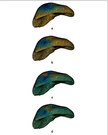
Fig. 8 First four spatial modes of the liver problem,Xk(x),k=1,. . .,4
The model, see Fig.7, is composed by 2853 nodes and 10,519 linear tetrahedra. For the ease exposition, a Kirchhoff-Saint Venant constitutive law with E = 160,000 Pa and ν = 0.48 is considered. More sophisticated constitutive laws are equally possible, see [7] and references therein. In Fig. 7 the region ¯ in which the load can be applied has been highlighted in red. Only 66 nodes have been chosen as candidates for load-ing, but of course even the entire surface of the organ can be chosen, as in [13], for instance.
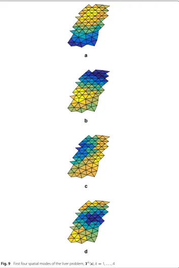
As in the previous example, the first four spatial and loading modesXk(x) andYk(s),
a
b
c
d
Fig. 9 First four spatial modes of the liver problem,Yk(s),k=1,. . .,4
The dual problem was solved by applying a stopping criterion such thatϕn+1−ϕn ≤ 10−8. The evolution of the predicted error with the number of modesnemployed in the
computation of the primal variable is shown in Fig.10.
Conclusions
0 20 40 60 1.35
1.4 1.45 1.5
·10−2
Number of PGD modes,n
o(e
)
Fig. 10 Convergence of the error with the number of modesnfor the liver problem
In this paper, we have developed a method for the error estimation in such a quantity of interest for a real-time simulator based on the use of reduced order models. In particular, proper generalized decomposition techniques have been employed.
Based on previous developments of the authors, an explicit linearization of the originally non-linear constitutive equations in the framework of PGD has been employed. This renders the problem in the form of a sequence of linear problems, for which an error estimator in the spirit of [34] has been employed. It is based on the employ of the so-called dual problem as a stopping criterion for the original (or primal) one.
The result is the first example (up to our knowledge) of an error estimator for non-linear problems in the framework of PGD methods in general, and haptic simulators in particular.
Authors’ contributions
IA, DG and SZ participated in the development of the proposed technique and implemented it in Matlab. PD, EC and FCh developed the technique, checked the results and wrote the manuscript. All authors read and approved the final manuscript.
Author details
1Aragon Institute of Engineering Research, Universidad de Zaragoza, María de Luna, s.n., 50018 Zaragoza, Spain, 2Laboratori de Càlcul Numèric, Universitat Politècnica de Catalunya, Jordi Girona 1-3, 08034 Barcelona, Spain,3GeM, Ecole
Centrale de Nantes, 1 rue de la Noe, 44321 Nantes, France.
Acknowledgements
This work has been supported by the Spanish Ministry of Economy and Competitiveness through Grant Numbers CICYT DPI2014-51844-C2-1-R and 2-R and by the Generalitat de Catalunya, Grant Number 2014-SGR-1471. This support is gratefully acknowledged.
Competing interests
The authors declare that they have no competing interests.
Received: 4 June 2015 Accepted 16 October 2015
References
1. Ghnatios C, Masson F, Huerta A, Leygue A, Cueto E, Chinesta F. Proper generalized decomposition based dynamic data-driven control of thermal processes. Comput Methods Appl Mech Eng. 2012;213–216:29–41. doi:10.1016/j.cma. 2011.11.018.
2. Bro-Nielsen M, Cotin S. Real-time volumetric deformable models for surgery simulation using finite elements and condensation. Comput Graph Forum. 1996;15(3):57–66.
4. Barbiˇc J, James DL. Real-time subspace integration for St. Venant–Kirchhoff deformable models. ACM Trans Graph (SIGGRAPH 2005) 2005;24(3):982–90.
5. Delingette H, Ayache N. Soft tissue modeling for surgery simulation. In: Ayache N, editor. Computational models for the human body. Handbook of Numerical Analysis (Ph. Ciarlet, Ed.). Amsterdam: Elsevier; 2004. p. 453–550. 6. Wang P, Becker AA, Jones IA, Glover AT, Benford SD, Greenhalgh CM, Vloeberghs M. Virtual reality simulation of
surgery with haptic feedback based on the boundary element method. Comput Struct. 2007;85(7–8):331–9. doi:10. 1016/j.compstruc.2006.11.021.
7. Cueto E, Chinesta F. Real time simulation for computational surgery: a review. Adv Model Simul Eng Sci. 2014;1(1):11. doi:10.1186/2213-7467-1-11.
8. Cotin S, Delingette H, Ayache N. Real-time elastic deformations of soft tissues for surgery simulation. In: Hagen H, editor. IEEE Transactions on Visualization and Computer Graphics vol. 5(1). IEEE Computer Society (1999). p. 62–73.
http://citeseer.ist.psu.edu/cotin98realtime.html.
9. Meier U, Lopez O, Monserrat C, Juan MC, Alcaniz M. Real-time deformable models for surgery simulation: a survey. Comput Methods Prog Biomed. 2005;77(3):183–97.
10. Taylor ZA, Cheng M, Ourselin S. High-speed nonlinear finite element analysis for surgical simulation using graphics processing units. IEEE Trans Med Imaging. 2008;27(5):650–63. doi:10.1109/TMI.2007.913112.
11. Miller K, Joldes G, Lance D, Wittek A. Total lagrangian explicit dynamics finite element algorithm for computing soft tissue deformation. Commun Numer Methods Eng. 2007;23(2):121–34. doi:10.1002/cnm.887.
12. Joldes GR, Wittek A, Miller K. Real-time nonlinear finite element computations on GPU—application to neurosurgical simulation. Comput Methods Appl Mech Eng. 2010;199(49–52):3305–14. doi:10.1016/j.cma.2010.06.037.
13. Niroomandi S, González D, Alfaro I, Bordeu F, Leygue A, Cueto E, Chinesta F. Real-time simulation of biological soft tissues: a PGD approach. Int J Numer Methods Biomed Eng. 2013;29(5):586–600. doi:10.1002/cnm.2544.
14. Niroomandi S, Alfaro I, Gonzalez D, Cueto E, Chinesta F. Real-time simulation of surgery by reduced-order modeling and x-fem techniques. Int J Numer Methods Biomed Eng. 2012;28(5):574–88. doi:10.1002/cnm.1491.
15. Niroomandi S, Gonzalez D, Alfaro I, Cueto E, Chinesta F. Model order reduction in hyperelasticity: a proper generalized decomposition approach. Int J Numer Methods Eng. 2013;96(3):129–49. doi:10.1002/nme.4531.
16. Gonzalez D, Cueto E, Chinesta F. Real-time direct integration of reduced solid dynamics equations. Int J Numer Methods Eng. 2014;99(9):633–53.
17. Chinesta F, Leygue A, Bordeu F, Aguado JV, Cueto E, Gonzalez D, Alfaro I, Ammar A, Huerta A. PGD-based compu-tational vademecum for efficient design, optimization and control. Arch Comput Methods Eng. 2013;20(1):31–59. doi:10.1007/s11831-013-9080-x.
18. Bernoulli C. Vademecum des Mechanikers. Cotta. 1836.http://books.google.es/books?id=j2dwQAAACAAJ. 19. Laughlin RB, Pines D. The theory of everything. Proc Natl Acad Sci. 2000;97(1):28–31. doi:10.1073/pnas.97.1.28.http://
www.pnas.org/content/97/1/28.full.pdf+html.
20. Ammar A, Mokdad B, Chinesta F, Keunings R. A new family of solvers for some classes of multidimensional partial differential equations encountered in kinetic theory modeling of complex fluids. J Non-Newtonian Fluid Mech. 2006;139:153–76.
21. Ladeveze P. Nonlinear computational structural mechanics. New York: Springer; 1999.
22. Chinesta F, Ladeveze P, Cueto E. A short review on model order reduction based on proper generalized decomposi-tion. Arch Comput Methods Eng. 2011;18:395–404.
23. Ladeveze P, Passieux J-C, Neron D. The latin multiscale computational method and the proper generalized decom-position. Comput Methods Appl Mech Eng. 2010;199(21–22):1287–96. doi:10.1016/j.cma.2009.06.023.
24. Chinesta F, Ammar A, Cueto E. Recent advances in the use of the proper generalized decomposition for solving multidimensional models. Arch Comput Methods Eng. 2010;17(4):327–50.
25. Allier P-E, Chamoin L, Ladeveze P. Proper generalized decomposition computational methods on a benchmark problem: introducing a new strategy based on constitutive relation error minimization. Adv Model Simul Eng Sci. 2015;2(1):17. doi:10.1186/s40323-015-0038-4.
26. Bouclier R, Louf F, Chamoin L. Real-time validation of mechanical models coupling pgd and constitutive relation error. Comput Mech. 2013;52(4):861–83. doi:10.1007/s00466-013-0850-y.
27. Rozza G, Huynh DBP, Patera AT. Reduced basis approximation and a posteriori error estimation for affinely para-metrized elliptic coercive partial differential equations. Arch Comput Methods Eng. 2008;15(3):229–75. doi:10.1007/ s11831-008-9019-9.
28. Huynh DBP, Rozza G, Sen S, Patera AT. A successive constraint linear optimization method for lower bounds of parametric coercivity and inf-sup stability constants. CR Math. 2007;345(8):473–8. doi:10.1016/j.crma.2007.09.019. 29. Stein E, Rüter M, Ohnimus S. Error-controlled adaptive goal-oriented modeling and finite element approximations
in elasticity. Comput Methods Appl Mech Eng. 2007;196(37–40):3598–613. doi:10.1016/j.cma.2006.10.032. Special Issue Honoring the 80th Birthday of Professor Ivo Babuška.
30. Meyer M, Matthies HG. Efficient model reduction in non-linear dynamics using the Karhunen-Loève expansion and dual-weighted-residual methods. Comput Mech. 2003;31(1–2):179–91. doi:10.1007/s00466-002-0404-1. 31. Hoang KC, Kerfriden P, Khoo BC, Bordas SPA. An efficient goal-oriented sampling strategy using reduced basis method
for parametrized elastodynamic problems. Numer Methods Partial Differ Equ. 2015;31(2):575–608. doi:10.1002/num. 21932.
32. Alastrue V, Calvo B, Pena E, Doblare M. Biomechanical modeling of refractive corneal surgery. J Biomech Eng Trans ASME. 2006;128:150–60.
33. Holzapfel GA, Gasser TC. A new constitutive framework for arterial wall mechanics and a comparative study of material models. J Elast. 2000;61:1–48.
34. Ammar A, Chinesta F, Diez P, Huerta A. An error estimator for separated representations of highly multidimensional models. Comput Methods Appl Mech Eng. 2010;199(25–28):1872–80. doi:10.1016/j.cma.2010.02.012.
36. Bouclier R, Louf F, Chamoin L. Real-time validation of mechanical models coupling PGD and constitutive relation error. Comput Mech. 2013;52(4):861–83. doi:10.1007/s00466-013-0850.
37. de Almeida JPM. A basis for bounding the errors of proper generalised decomposition solutions in solid mechanics. Int J Numer Methods Eng. 2013;94(10):961–84. doi:10.1002/nme.4490.