Wine grape cultivar influence on the performance of models that predict the lower threshold canopy temperature of a water stress index

(1)

Contents lists available atScienceDirect

Computers and Electronics in Agriculture

journal homepage:www.elsevier.com/locate/compag

Original papers

Wine grape cultivar in

ﬂ

uence on the performance of models that predict the

lower threshold canopy temperature of a water stress index

B.A. King

a,⁎

, K.C. Shellie

b

a_{USDA ARS, Northwest Irrigation and Soils Research Unit, 3793 N 3600 E, Kimberly, ID 83341, United States} b_{USDA ARS, HCRU Corvallis, OR-Parma, ID Worksite, 29603 U of I Lane, Parma, ID 83660, United States}

A R T I C L E I N F O

Keywords:

Modeling Neural network Crop water stress index Deﬁcit irrigation

Vitis vinifera

A B S T R A C T

The calculation of a thermal based Crop Water Stress Index (CWSI) requires an estimate of canopy temperature under non-water stressed conditions (Tnws). The objective of this study was to assess the inﬂuence of diﬀerent wine grape cultivars on the performance of models that predict Tnws. Stationary infrared sensors were used to

measure the canopy temperature of the wine grape cultivars Malbec, Syrah, Chardonnay and Cabernet franc under well-watered conditions over multiple years and modeled as a function of climatic parameters–solar radiation, air temperature, relative humidity and wind speed using multiple linear regression and neural net-work modeling. Despite diﬀerences among cultivars inTnws, both models provided good prediction results when

all cultivars were collectively modeled. For all cultivars, prediction error variance was lower in neural network models developed from cultivar-specific datasets than regression models developed from multi-cultivar datasets. Overall, the cultivar-specific models had less prediction error variance than multi-cultivar models. Multi-cultivar models generally resulted in prediction bias whereas cultivar-specific models eliminated the prediction bias. All predictive models had an uncertainty of ± 0.1 in calculation of the CWSI despite significantly different pre-diction error variance between models.

1. Introduction

Wine grapes (Vitis viniferaL.) are widely grown in arid and semiarid regions where irrigation is used to supplement annual precipitation. The desired amount of water to supply during an irrigation event is usually less than estimated vine water demand (ETc), with the goal of inducing some vine water stress to manage vegetative growth, induce beneficial changes in berry composition (Sadras and Moran, 2012), and increase water productivity (Shellie, 2014; Chaves et al., 2007; Fereres and Soriano, 2007). Decisions about when to irrigate and how much water to supply during an irrigation event ultimately influence pro-duction profitability in terms of input costs, yield and fruit quality. The Penman-Monteith model is commonly used to estimate how much water to supply during an irrigation event (Allen et al., 1998). The model estimates vine water demand (ETc) from the evapotranspiration of a reference crop (ETr), a crop specific coefficient (Kcb), and a stress coefficient (Ks) to account for a decrease in water demand when tran-spiration is restricted by unfavorable environmental conditions. The equation for estimating ETcunder transpiration-limiting conditions is:

=

− K K

ETc adj ET (r cb s) (1)

If the value of Ksrepresents the amount of transpiration being limited by a water deficit, the value ofKscould serve as a guide for irrigation scheduling. However, determining a reliable value for Kshas been difficult. The methods commonly used to monitor vine water status, such as soil moisture or plant water potential, often have poor spatial and temporal resolution or are too laborious for automation. Also, wine grape cultivars are known to differ in their hydraulic be-havior and alter their usual bebe-havior under different environmental conditions (Pou et al., 2012; Chaves et al., 2010; Lovisolo et al., 2010; Vandeleur et al., 2009). This poses an additional level of difficulty in estimatingKs. For example,Hochberg et al. (2017)supplied the same fractional amount of ETcto different wine grape cultivars under iden-tical environmental conditions and reported differing levels of vine water stress severity among cultivars and higher or lower than intended severities of water stress at different vine phenological stages. This suggests that Ks values may differ according to cultivar and to the phenological stage of vine development.

Thermal remote sensing has been used to estimate drought stress in many crops, including grapevine (Maes and Steppe, 2012). An em-pirical crop water stress index (CWSI) was developed byJackson et al. (1981)andIdso et al. (1981)to indirectly estimateKs.Jackson (1982)

https://doi.org/10.1016/j.compag.2017.12.025

Received 21 September 2017; Received in revised form 13 December 2017; Accepted 15 December 2017

⁎_{Corresponding author.}

E-mail addresses:[email protected](B.A. King),[email protected](K.C. Shellie).

(2)

comparedin situmeasurements of leaf temperature with soil volumetric water content and found leaf temperature to be a more reliable in-dicator of plant water status. The equation used to calculate the CWSI is:

= −

−

CWSI T T

T T

( )

canopy nws

dry nws (2)

whereTcanopyis the measured temperature of the vine canopy, andTdry andTnwsare the upper and lower canopy temperature thresholds when transpiration is completely limited or non-restricted, respectively. The CWSI ranges in value from 0 to 1 where 0 indicates optimum conditions for maximum transpiration (Tnws) and 1 represents a non-transpiring condition (Tdry). The need for an irrigation event is signaled when the CWSI value exceeds a desired numerical threshold. The CWSI (Colaizzi et al., 2003) and the ratio ofTcanopytoTnws(Bausch et al., 2011) have been used in cotton and corn, respectively, to guide irrigation sche-duling and indirectly estimateKsfor determining ETc.

The CWSI has been of limited use with wine grapes due to the practical difficulty of determining values for Tnws and Tdrywhile si-multaneously measuringTcanopy(Jones et al., 2002). Approaches that have been used to estimate Tnws include energy balance equations (Sepúlveda-Reyes et al., 2016; Möller et al., 2007) natural or artificial reference surfaces (Sepúlveda-Reyes et al., 2016; Pou et al., 2014; Möller et al., 2007), and the difference in temperature betweenTcanopy and air relative to evaporative demand (Bellvert et al., 2015; Idso et al., 1981). A constant has been used to estimate a value forTdry(Möller et al., 2007; King and Shellie, 2016). The influence of cultivar hydraulic behavior on the accuracy of these approaches has not been evaluated. King and Shellie (2016) predicted lower canopy temperature threshold values for the wine grape cultivars Syrah and Malbec using a neural network (NN) model developed from cultivar-specific datasets. The importance of cultivar specificity in the dataset used to train, test and validate the NN predictive model was not evaluated. The objective of this research was to ascertain the influence of cultivar on model predictive performance. Under well-wateredfield conditions, we con-tinuously monitored the canopy temperature of grape cultivars Ca-bernet franc (CF), Chardonnay (CH), Malbec (MB) and Syrah (SY) over consecutive growing seasons and used the measured temperatures to develop neural network (NN) and multiple linear regression models to predict Tnws. Cultivar influences were indirectly evaluated by com-paring the predictive performance of models developed from a cultivar-specific dataset to that of models developed from a multi-cultivar da-taset.

2. Materials and methods

2.1. Trial site and irrigation

This study was conducted over three growing seasons (2014, 2015, and 2016) in three experimental vineyards located at the University of Idaho Parma Research and Extension Center in Parma, ID (lat. 43°37′7.9716″N, long. 116°12′54.1″W, 750 m asl). Two of the vineyards were located adjacent to one another and were planted in 2007 with un-grafted, dormant-rooted cuttings of either MB or SY. The other vineyard was located ∼0.5 km southeast of the MB and SY trial sites and was planted in 1997 with un-grafted, dormant-rooted cuttings of CF and CH. Vines in all three vineyards were managed according to local com-mercial practices (double-trunked, bilateral cordon, spur-pruned an-nually to 16 buds/m of cordon, vertically positioned on a two-wire trellis with moveable wind wires). The vineyards are described in more detail byShellie (2007)andKing and Shellie (2016).

The vineyards were irrigated toﬁeld capacity each year prior to bud break to encourage uniform bud break and at the end of the growing season to reduce the risk of freeze injury. Vines were also drip-irrigated 3–5 times a week with an amount of water estimated to meet or exceed

Table 1

Climate data from 1 Apr through 31 Oct collected at the PMAI weather station located 3 km from the research vineyards in Parma, ID [(www.usbr.gov/pn/agrimet/), latitude 43°48′00″, longitude 116°56′00″, elevation 702 m] and amount of irrigation water sup-plied during berry development.

2014 2015 2016 1994–2012 average

Precipitation (mm) 88 113 120 99.6 ± 35 Daily average total direct solar

radiation (MJ m−2₎

22.3 21.9 22.6 22.1 ± 0.9

Days daily maximum temperature exceeded 35 °C

27 25 26 28 ± 12

Z_{Accumulated growing degree days}

(°C)

1759 1865 1688 1708 ± 115

Alfalfa-based reference

evapotranspiration (ETr) (mm)

1314 1265 1329 1212 ± 55

Irrigation amount (mm)

Syrah 726 514 1322

Malbec 521 514 973

Cabernet franc NE 599 1369 Chardonnay NE 599 1369

Z_{Accumulated growing degree days were calculated from daily maximum and}

minimum temperature with no upper limit and a base temperature of 10 °C.

Table 2

Least square mean values for midday leaf water potential (Ψmd) of vines drip-irrigated to

supply estimated vine water demand (ETc) from fruit set until harvest. Vines were grown

inﬁeld plots in a research vineyard in Parma, ID and measured weekly on a day preceding an irrigation event.

Preveraison (MPa) Postveraisona_(MPa)

−0.84

Year 2014b _−0.75b

2015 −0.88c

2016 −0.55a

Cultivar Syrah −0.73b

Malbec −0.73b

Cabernet franc −0.86a

Chardonnay −0.81ab

pvaluesc

Preveraison Postveraison

Year ns **

CV ns *

Year * CV ns ns

a_{Same lowercase letter within a treatment level column indicates no signiﬁcant}

dif-ference atp≤.05 by Tukey-Kramer adjustedttest.

b_{Analysis excludes cultivars Cabernet franc and Chardonnay.} c *_,**_{, and ns indicate}_p_{≤.05, 0.01, and not signiﬁcant, respectively.}

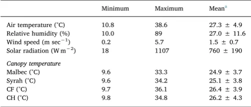
Table 3

Minimum and maximum values for vineyard environmental conditions and well-watered canopy temperatures measured between 13:00 and 15:00 MDT in Parma, ID in 2014 (26 June through 6 Oct), 2015 (25 June 25 through 23 Sept), and 2016 (23 June through 27 Sept) and used to linearly scale Neural Network input parameters.

Minimum Maximum Meana

Air temperature (°C) 10.8 38.6 27.3 ± 4.9 Relative humidity (%) 10.0 89 27.0 ± 11.6 Wind speed (m sec−1₎ _0.2 _5.7 _{1.5 ± 0.7}

Solar radiation (W m−2₎ ₁₈ ₁₁₀₇ _{760 ± 190}

Canopy temperature

Malbec (°C) 9.6 33.3 24.9 ± 3.7 Syrah (°C) 9.6 34.2 25.1 ± 3.8

CF (°C) 9.7 36.1 26.4 ± 3.9

CH (°C) 9.8 34.8 26.2 ± 4.3

(3)

ETcbeginning when berries were∼7 mm in diameter at growth stage 31 of the modiﬁed E-L grapevine growth stage system (Coombe, 1995) and continuing until harvest at fruit maturity. The Penman-Monteith model (Allen et al., 1998) was used to estimate ETcwithKcbincreasing during canopy development from 0.3 to 0.7 and Ks= 1. Alfalfa re-ference crop (ETr) values were obtained from a weather station located 3 km from the study location (http://www.usbr.gov/pn/agrimet/ wxdata.html). Midday leaf water potential (Ψmd) was checked weekly to ensure a value less negative than−1.0 MPa, a threshold below which was previously observed to restrict shoot growth (Shellie, 2006). Irri-gation delivery amount was recorded usingﬂow meters.

2.2. Plant water status measurements

Vine water status was monitored weekly throughout berry devel-opment by measuring leaf water potential at midday (Ψmd) using a pressure chamber1_{(model 610; PMS Instruments, Corvallis, OR)} fol-lowing the method of Turner (1988)as described byShellie (2006). Two, fully expanded, sunlit leaves were measured per vine in two vines per cultivar. WeeklyΨmdpre- and postveraison measurements collected were analyzed by phenological stage using a repeated measure analysis of variance (ANOVA) with cultivar as afixed effect and years as a re-peated measure (ver. 9; SAS Institute, Cary NC). The probability of a significant difference among treatment levels (p≤.05) was determined using the Tukey-Kramer adjustedttest. Seasonal cumulative growing degree days were calculated from daily minimum (base threshold of 10 °C) and maximum (no upper limit) temperatures recorded at the nearby weather station (http://www.usbr.gov/pn/agrimet/wxda-ta.html) from 1 Apr to 31 Oct.

2.3. Measurement of canopy temperature and vineyard environmental conditions

Stationary infrared temperature sensors (SI-121 Infrared radio-meter; Apogee Instruments, Logan, UT) were positioned approximately 15 to 30 cm over the top of the vine canopy (viewing 2–5 leaves) and used to measure canopy temperature as described byKing and Shellie (2016). Two infrared temperature sensors were installed for each cul-tivar, with each sensor located on a diﬀerent vine. The leaf temperature sensing area was approximately 15–30 cm in diameter and the center of ﬁeld of view was aimed at the center of leaves receiving full sunlight exposure during midday.

The environmental conditions monitored in the vineyard were: wind speed (WS) (05305 anemometer, R.M. Young, Traverse City, MI), air temperature (Tair), relative humidity (RH) (HMP50 temperature and humidity probe, Campbell Scientiﬁc, Logan, UT), and solar radiation (SR) (LI-200SZ pyranometer, LI-COR Biosciences, Lincoln, NE). Environmental sensors were located in the vine row, above the grape-vine canopy withTair,RHandSRmeasured at 2.2 m andWSmeasured at 2.5 m above ground level, as described byKing and Shellie (2016). Wind speed was adjusted to a standard height of 2 m (Allen et al., 1998).

Environmental conditions and vine canopy temperatures were concurrently measured continuously between grapevine growth stage 31 (berries 7 mm diameter) and stage 38 (berries harvest-ripe) (Coombe, 1995). Data were measured at 1-min intervals and recorded as 15-min average values on a datalogger, as described by Shellie and King (2016). Canopy temperature and environmental data were col-lected in 2014 from 26 June through 6 Oct; in 2015, from 2 July through 23 Sept; and in 2016, from 7 July through 27 Sept. The canopy temperatures of Syrah and Malbec were measured in all three study

years and that of CH and CF were measured in 2015 and 2016.

2.4. Datasets and Tnwspredictive models

The entire, multiyear dataset wasfiltered to include only data re-corded between 13:00 and 15:00 MDT ( ± 90 min around solar noon), as described byKing and Shellie (2016). Time of solar noon at the study site ranged from 13:53 to 13:35 MDT over the measurement dates in each year. Thefiltered dataset was subdivided to create two unique datasets for each cultivar. One dataset contained only the measured temperatures for a specific cultivar (cultivar-specific) and the other dataset contained all the measured temperatures in thefiltered dataset for the three remaining cultivars (multi-cultivar). Each dataset con-tained the measured canopy temperatures and the corresponding vi-neyard environmental conditions (SR,Tair, RH, WS) recorded at the time of canopy temperature measurement. The cultivar-specific and multi-cultivar dataset for each cultivar was used to develop a neural network (NN) model and a multiple linear regression model to predict

Tnws. The same environmental data and measured canopy temperatures were used as input parameters for both model types. MATLAB Neural Network Toolbox software (MathWorks, Natick, MA) was used to de-velop the NN models and Microsoft Excel was used to dede-velop the multiple linear regression models. Each NN model was trained, tested and validated by subdividing the dataset into three parts, each of which contained 70, 15, and 15% of the total dataset, respectively. Neural network model input parameters were linearly scaled to a range of−1 to 1 based upon the maximum and minimum values for the measured parameter. The Levenberg-Marquardt back propagation method (Haykin, 2009) was used to train the network with the training dataset. A multilayer perceptron feed forward NN architecture was used. Hidden layer neurons and the single output neuron used a hyperbolic tangent activation function. The NN models had one hidden layer with ﬁve neurons.

2.5. Model predictive performance

For each cultivar, the predictive performance of models developed from cultivar-specific datasets was compared to models developed from multi-cultivar datasets. Model predictive performance was compared by goodness offit parameters mean square error (MSE), model efficiency (ME) and percent bias (PBIAS). The MSE is a measure of the amount of error between predicted and observed values. The MSE was calculated as:

= ⎡ ⎣ ⎢

∑ − _⎤

⎦ ⎥

O P n

MSE ( i i)

2

(3) whereOiwas the observedith data value,Piwas the predictedith data value, andnwas the number of data values. Values for MSE range from 0.0 to∞, with an optimal value of zero. A model with a lower MSE is more accurate than a model with a higher MSE. Model efficiency (ME) is analogous to the common correlation coefficient for linear regression. Model efficiency was calculated as:

= −⎡ ⎣ ⎢

∑ −

⎤

⎦ ⎥

O P O O

ME 1 ( )

( )

i i

i avg 2

2

(4) where Oavgis the average value of all measuredOidata values (Nash and Sutcliffe, 1970). Values of ME range from−∞to an optimal value of 1.0. A value of zero indicates that the values predicted by the model are no more accurate than the mean value of the observed data. The ME is not based upon the proportion of variation explained by a regres-sion’s independent variable, so its value can be < 0 if the data set contains extreme values, a non-linear function isfit to observed data, or model predicted values are less accurate than the mean of the observed values. The PBIAS is a measure of how much thefitted model over or under predicted the observed values. The PBIAS was calculated as

1_{The mention of trade names of commercial products in this article is solely for the}

(4)

(Yapo et al., 1996):

= ⎡ ⎣ ⎢

∑ −

∑ ⎤ ⎦ ⎥

P O O

PBIAS ( )

( ) (100)

i i

i (5)

Values for PBIAS range from−∞to∞with an optimal value of zero; however, values close to zero can occur if theﬁtted model over predicts as much as it under predicts (Moriasi et al., 2007).

Model performance was also evaluated by statistical analysis of the variance of model prediction errors. Model prediction performance is inversely related to the magnitude of the variance of model prediction errors. Normal Q-Q plots, histograms, and Shapiro-Wilk’s test (p≤.05) and Kolmogorov-Smirnov test (p≤.05) were used to ascertain whether prediction errors were approximately normally distributed. Equality of variances for normally distributed data were evaluated using a Levine test and, for data not normally distributed, using a non-parametric Levine test (Nordstokke and Zumbo, 2010; Nordstokke et al., 2011).

Multiple comparisons of variance were tested using the Bonferroni correction to minimize the likelihood of incorrectly rejecting a null hypothesis (Type I error).

The inﬂuence of model prediction error on error distribution of the CWSI was estimated for the cultivar SY using Monte Carlo simulation in an Excel spreadsheet to calculate the CWSI as:

= −

−

CWSI error T T T T

( )

mnws pnws

dry pnws (6)

where Tpnwsis the model predicted canopy temperature when measured (assumed known) canopy temperature (Tmnws) was 26 °C and Tdrywas 44 °C (29 °C air temperature +15 °C) (King and Shellie, 2016). Values for Tpnwswere obtained from the linear regression model developed from the multi-cultivar dataset and the NN model developed from the cultivar-speciﬁc dataset. Model prediction error variances were as-sumed to be approximately normally distributed for simulation pur-poses. Graphs inﬁgures were generated using Sigmaplot 11.2 (Systat Software, San Jose, CA).

3. Results and discussion

3.1. Vineyard environmental conditions

Growing season precipitation, solar radiation and the number of days that the daily maximum temperature exceeded 35 °C was similar each year to the 19-year site average (Table 1). In 2014 and 2016, accumulated growing degree days (GDD) were similar and reference evapotranspiration (ETr) was greater than the 19-year site average. In 2015, GDD were greater and ETrwas similar to the 19-year site average. The amount of irrigation water supplied during berry development

Table 4

Prediction error variances for neural network (NN) and multiple linear regression (REG) models developed to predict the well-watered canopy temperature of grapevine cultivars Malbec, Syrah, Cabernet franc (CF) and Chardonnay (CH) using multi-cultivar and cul-tivar-speciﬁc datasets.

Model Dataset Malbeca _Syrah _CF _CH _{All cultivars}

NN Multi-cultivar 1.40ab 1.08bc 1.14a 0.89c 1.25a NN Cultivar-speciﬁc 1.23b 0.88c 0.75b 0.77c NE REG Multi-cultivar 1.64a 1.33a 1.21a 1.13a 1.46a REG Cultivar-speciﬁc 1.56ab 1.20b 0.97a 1.05b NE

a_{Variances with the same letter within a cultivar column are not signiﬁcantly diﬀerent}

using the Bonferroni correction for multiple pair-wise comparisons (p≤.01).

Predicted T

nws

(deg C)

5 10 15 20 25 30 35

Measured T_nws (deg C) Measured T_nws (deg C)

5 10 15 20 25 30

Predicted T

nws

(deg C)

5 10 15 20 25 30

5 10 15 20 25 30 35

Multi-cultivar Regression

ME= 0.87 PBIAS = 1.6 MSE = 1.6

ME= 0.89 PBIAS = 0.0 MSE = 1.6

ME= 0.89 PBIAS = 1.7 MSE = 1.8

ME= 0.91 PBIAS = 0.0 MSE = 1.2 Cultivar-specific Regression

Multi-cultivar Neural Network

Cultivar-specific Neural Network

(5)

relative to ETr was ∼53% in 2014 and 2015 and ∼94% in 2016 (Table 1).

Pre- and post-veraisonΨmdwas less negative than−1.0 MPa in all cultivars each year (Table 2). PreveraisonΨmdwas similar each year among cultivars and among years. PostveraisonΨmdwas least negative in 2016 and most negative in 2014. The postveraisonΨmdof CF was more negative than that of SY and MB and similar to that of CH.

The maximum and minimum values recorded between 13:00 and 15:00 MDT in 2014 used to linearly scale input parameters for the NN model are presented inTable 3. Minimum and maximum canopy tem-peratures were always cooler than ambient air temtem-peratures and the magnitude of the diﬀerence varied among cultivars. The diﬀerence between vine canopy temperature and ambient air was greatest (∼4.0 °C) when air temperature was warmest. When ambient air tem-perature was coolest, vine canopy temtem-perature was an average of 1.1 °C cooler. Malbec had the coolest and CF had the warmest maximum ca-nopy temperature. The range among cultivars in minimum and max-imum canopy temperature was 0.2 and∼3 °C, respectively.

3.2. Model predictive performance for Tnwsfor diﬀerent cultivars

For each of the four cultivars, the models developed from a multi-cultivar dataset tended to have higher prediction error variance than the models developed from a cultivar-specific dataset (Table 4). For models developed using the multi-cultivar dataset, the prediction error variance of the NN model was lower than that of the regression model for each of the four cultivars; however, the difference was of statistical significance only for SY and CH. When a cultivar-specific dataset was used for model development, the NN model had lower prediction error variance than the regression model; however, the difference was of

statistical signiﬁcance only for CF.

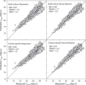
The relative performance of model parameters among the four models that were developed for each cultivar differed by cultivar. For the cultivar MB, the ME was similar among the four models; however, models developed from the cultivar-specific dataset had the lowest PBIAS (Fig. 1). The positive bias of the multi-cultivar datasets suggests that MB had a lower Tnwsthan other cultivars in the multi-cultivar dataset. The cultivar-specific regression model shows a visual positive bias when Tnws< 20 °C and a negative bias when Tnws> 25 °C, which tend to balance resulting in a zero bias. This bias was not visually ap-parent in the cultivar-specific NN model. The cultivar-specific NN model had the lowest MSE and had significantly less prediction error variance relative to the multi-cultivar regression model (Table 4).

There was a wider range in ME among the models developed for SY than among the models developed for MB (Fig. 2). The NN model had a higher ME than the regression model developed from the same dataset. The cultivar-specific NN model had the highest ME. The PBIAS was highest in models developed from the multi-cultivar dataset. The po-sitive bias of both multi-cultivar datasets suggests that SY, like MB, had a lower Tnwsthan other cultivars in the multi-cultivar dataset. Syrah and MB also had similar and less negative postveraisonΨmdthan CH and CF (Table 2). The cultivar-specific NN model had the lowest MSE. The multi-cultivar regression model had the highest MSE and highest prediction error variance (Table 4). The cultivar-specific NN model had lower prediction error variance than either of the regression models.

For CF, the multi-cultivar developed models had lower ME, greater PBIAS and higher MSE than the cultivar speciﬁc models and there was little performance diﬀerence between the NN and regression model developed from each dataset (Fig. 3). The PBIAS of the multi-cultivar models was negative suggesting that CF has a higher Tnwsthan other

Predicted T

nws

(deg C)

5 10 15 20 25 30 35

Measured T_nws (deg C)

5 10 15 20 25 30

Predicted T

nws

(deg C)

5 10 15 20 25 30

5 10 15 20 25 30 35

ME= 0.88 PBIAS = 2.2 MSE = 1.6

ME= 0.91 PBIAS = 0.0 MSE = 1.2

ME= 0.90 PBIAS = 2.2 MSE = 1.4

(6)

cultivars in the multi-cultivar dataset. The cultivar-speciﬁc NN model had lower prediction error variance than any of the other models (Table 4).

The relative difference in performance among models developed for CH was similar to that of CF (Fig. 4). The multi-cultivar developed models had lower ME, greater PBIAS and higher MSE than the cultivar specific models and there was little performance difference between the NN and regression model developed from each dataset. The negative PBIAS of the multi-cultivar models suggests that the Tnwsof CH, like CF, was higher than that of other cultivars in the multi-cultivar dataset. The postveraisonΨmdof CH and CF also was similar and was more negative than SY and MB (Table 2). The cultivar-specific regression model for CH had a visual positive bias for Tnws< 20 °C and negative bias for Tnws> 20 °C, which tend to balance resulting in a zero bias and greater MSE than the cultivar specific NN model. Both of the NN models had lower prediction error variances than either of the regression models (Table 4).

Prediction error for Tnwsintroduces uncertainty in the calculation of the CWSI since Tnwsis used in both the numerator and denominator of Eq.(2). To estimate the practical importance of prediction error var-iance on the calculation of the CWSI, the propagation of Tnwsprediction error uncertainty was investigated for the cultivar SY using Monte Carlo simulation (Eq.(3)). The importance of error variance on calculation of the CWSI was evaluated by comparing the distribution of a CWSI value about zero when Tnwswas predicted using the multi-cultivar regression model (prediction error variance of 1.33) to when Tnwswas predicted using the cultivar-speciﬁc NN model (prediction error variance of 0.88) (Table 4). When the multi-cultivar regression model was used to predict Tnws, the calculated CWSI was ± 0.05 and ± 0.1 from the true value of zero 55 and 86 percent of the time (Fig. 5). When the cultivar-speciﬁc

NN model was used to predict Tnws, the calculated CWSI was ± 0.05 and ± 0.1 from zero 63 and 93 percent of the time. The lower predic-tion error variance of the NN model reduced uncertainty by less than 10%. For both models, Tnwsprediction error resulted in an uncertainty of ± 0.1 in calculation of CWSI, even for the model with the lowest ME. When theﬁltered dataset that included all cultivars and years was used for model development, the NN and regression models had statistically similar prediction error variance, even though the error variance of the NN model was lower by∼14% (Table 4). Both of the models developed from theﬁltered dataset had similar ME and a low PBIAS; however, the NN model had a lower MSE (Fig. 6).

The higher prediction error variance of models developed from the filtered and multi-cultivar datasets is likely a reflection of inherent differences in Tnwsamong cultivars. Other indicators that Tnwsdiffered by cultivar were the higher PBIAS of multi-cultivar relative to cultivar-specific models, differences in postveraisonΨmd(Table 2) and diff er-ences in maximum and minimum canopy temperatures (Table 3). The cultivar differences in Tnws across climatic conditions introduced a substantial amount of variance in predicted Tnws. The hydraulic beha-vior of SY, CH and CF has been described as near-anisohydric whereas MB has been described as isohydrodynamic (Lovisolo et al., 2010; Shellie and Bowen, 2014). The influence of vapor pressure deficit on stomatal conductance under high and low soil moisture conditions has been reported to differ between isohydric and anisohydric cultivars (Domec and Johnson, 2012; Hochberg et al., 2017). From a practical point of view, a regression model developed from a large multi-cultivar database is likely to provide as accurate an estimate of Tnwswith less computational requirements as a NN model.

Predicted T

nws

(deg C)

5 10 15 20 25 30 35

Measured Tnws (deg C)

5 10 15 20 25 30

Predic

ted Tnws

(deg C)

5 10 15 20 25 30

5 10 15 20 25 30 35

ME= 0.92 PBIAS = -2.1 MSE = 1.5

ME= 0.95 PBIAS = 0.0 MSE = 1.0

ME= 0.92 PBIAS = -2.3 MSE = 1.5

ME= 0.96 PBIAS = -0.1 MSE = 0.8 Cultivar-specific Regression

(7)

4. Conclusions

The canopy temperature of the wine grape cultivars MB, SY, CH, and CF were measured under well-watered conditions over multiple

years and modeled as a function of climatic parameters - solar radia-tion, air temperature, relative humidity and wind speed using multiple linear regression and neural network modeling. Both models provided good prediction results when all cultivars are collectively modeled with

Predicted T

nws

(deg C)

5 10 15 20 25 30 35

5 10 15 20 25 30

Predicted T

nws

(deg C)

5 10 15 20 25 30

5 10 15 20 25 30 35

ME= 0.90 PBIAS = -2.5 MSE = 1.6

ME= 0.93 PBIAS = 0.0 MSE = 1.0

ME= 0.91 PBIAS = -2.7 MSE = 1.4

Fig. 4.Neural network and regression model perfor-mance values for predicting the non-water stressed canopy temperature (Tnws) of the cultivar Chardonnay (CH) developed from the multi-cultivar dataset or a data subset that contained only the measuredTnwsfor cultivar CH.

Crop Water Stress Index

-0.275 -0.225 -0.175 -0.125 -0.075 -0.025 0.025 0.075 0.125 0.175 0.225 0.275

Probability

0.00 0.05 0.10 0.15 0.20 0.25 0.30 0.35

1.33 0.88

Prediction Error Variance

Fig. 5.Inﬂuence of Syrah Tnwsmodel prediction error

on the distribution of calculated crop water stress index (CWSI) values for a known Tnwsvalue of 26 °C,

(8)

minimal predictive difference between the models. The performance of models developed from cultivar-specific or multi-cultivar datasets were compared to investigate the influence of cultivar differences on model predictive performance. For all cultivars, prediction error variance was lower in NN models developed from cultivar-specific datasets than re-gression models developed from multi-cultivar datasets. Overall, the cultivar-specific models had less prediction error variance than multi-cultivar models. Multi-multi-cultivar models generally resulted in prediction bias whereas cultivar-specific models eliminated the prediction bias. The effect of model prediction error on uncertainty in calculation of the CWSI was evaluated using Monte Carlo simulation. In general, all models result in an uncertainty of ± 0.1 in calculation of CWSI despite having significantly difference prediction error variance between models and a good estimate of well-watered canopy temperature (ME > 0.85).

Acknowledgements

This work was supported by the Idaho Department of Agriculture Specialty Crop Block Grant [grant number #14-SCBGP-ID-0016, 2014].

References

Allen, R.G., Pereira, L.S., Raes, D., Smith, M., 1998. Crop Evapotranspiration-Guidelines for Computing Crop Water Requirements-FAO Irrigation and Drainage Paper 56.

Food Agricultural Organization, Rome.

Bausch, W., Trout, T., Buchleiter, G., 2011. Evapotranspiration adjustments for deﬁ

cit-irrigated corn using canopy temperature: a concept. Irrig. Drain. 60, 628–693.

Bellvert, J., Marsal, J., Girona, J., Zarco-Tejada, P.J., 2015. Seasonal evolution of crop water stress index in grapevine varieties determined with high-resolution remote

sensing thermal imagery. Irrig. Sci. 33, 81–93.

Chaves, M.M., Santos, T.P., Souza, C.R., Ortuño, M.F., Rodrigues, M.L., Lopes, C.M.,

Maroco, J.P., Pereira, J.S., 2007. Deﬁcit irrigation in grapevine improves water-use

eﬃciency while controlling vigour and production quality. Ann. Appl. Biol. 150,

237–252.

Chaves, M.M., Zarrouk, O., Fransisco, R., Costa, J.M., Santo, T., Regalado, A.P.,

Rodrigues, M.L., Lopes, C.M., 2010. Grapevine under deﬁcit irrigation: hints from

physiological and molecular data. Ann. Bot. 105, 661–676.

Colaizzi, P.D., Barnes, E.M., Clarke, T.R., Choi, C.Y., Waller, P.M., 2003. Estimating soil moisture under low frequency surface irrigation using crop water stress index. J.

Irrig. Drain. Eng. ASCE 129, 36–43.

Coombe, B.G., 1995. Growth stages of the grapevine. Austral. J. Grape Wine Res. 1,

100–110.

Domec, J.C., Johnson, D.M., 2012. Does homeostasis or disturbance of homeostasis in minimum leaf water potential explain the isohydric versus anisohydric behavior of

Vitis viniferaL. cultivars? Tree Physiol. 32, 245–248.

Fereres, E., Soriano, M.A., 2007. Deﬁcit irrigation for reducing agricultural water use. J.

Exp. Bot. 58, 147–159.

Haykin, S., 2009. Neural Networks and Learning Machines. Pearson Education, Inc.,

Upper Saddle River, NJ0-13-147139-2.

Hochberg, U., Herrera, J.C., Degu, A., Castellarin, S.D., Peterlunger, E., Alberti, G., Lazarovitch, N., 2017. Evaporative demand determines the relative transpirational

sensitivity of deﬁcit-irrigated grapevines. Irrig. Sci. 35, 1–9.

Idso, S.B., Jackson, R.D., Pinter Jr, P.J., Reginato, R.J., Hatﬁeld, J.L., 1981. Normalizing

the stress-degree-day parameter for environmental variability. Agric. Meteorol. 24,

45–55.

Jackson, R., 1982. Canopy temperature and crop water stress. Adv. Irrig. 1, 43–85.

Jackson, R.D., Idso, S.B., Reginato, R.J., Pinter Jr, P.J., 1981. Canopy temperature as a

drought stress indicator. Water Resour. Res. 13, 651–656.

Jones, H.G., Stroll, M., Santos, T., de Sousa, C., Chaves, M.M., Grant, O.M., 2002. Use of

infrared thermography for monitoring stomatal closure in theﬁeld: application to

grapevine. J. Exp. Bot. 53, 2249–2260.

King, B.A., Shellie, K.C., 2016. Evaluation of neural network modeling to predict non-water-stressed leaf temperature in wine grape for calculation of crop water stress

index. Agric. Water Manag. 167, 38–52.

Lovisolo, C., Perrone, I., Carra, A., Ferrandino, A., Flexas, J., Medrano, H., Shubert, A.,

2010. Drought-induced changes in development and function of grapevine (Vitisspp.)

organs and in their hydraulic and non-hydraulic interactions at the whole-plant level:

a physiological and molecular update. Funct. Plant Biol. 30, 607–619.

Maes, W.H., Steppe, K., 2012. Estimating evapotranspiration and drought stress with ground-based thermal remote sensing in agriculture: a review. J. Exp. Bot. 63,

4671–4712.

Möller, M., Alchanatis, V., Cohen, Y., Meron, M., Tsipris, J., Naor, A., Ostrovsky, V., Sprintsin, M., Cohen, S., 2007. Use of thermal and visible imagery for estimating crop

water status of irrigated grapevine. J. Exp. Bot. 58, 827–838.

Moriasi, D.N., Arnold, J.G., Van Liew, M.W., Bingner, R.L., Harmel, R.D., Veith, T.L.,

2007. Model evaluation guidelines for systematic quantiﬁcation of accuracy in

wa-tershed simulations. Trans. ASABE 50 (3), 885–900.

Nash, J.E., Sutcliﬀe, J.V., 1970. Riverﬂow forecasting through conceptual models of

principles. J. Hydrol. 10 (1), 282–290.

Nordstokke, D.W., Zumbo, B.D., 2010. A new nonparametric Levene test for unequal

variances. Psicológica 32, 401–430.

Nordstokke, D.W., Zumbo, B.D., Cairns, S.L., Saklofske, D.H., 2011. The operating char-acteristics of the nonparametric Levene test for unequal variances with assessment

and evaluation data. Pract. Assess., Res. Evaluat. 16 (5), 1–8.

Pou, A., Medran, H., Tomás, M., Martorell, S., Ribas-Carbó, M., Flexas, J., 2012. Anisohydric behavior in grapevines results in better performance under moderate

water stress and recovery than isohydric behavior. Plant Soil 359, 335–349.

Pou, A., Diago, M.P., Medrano, H., Baluja, J., Tardaguila, J., 2014. Validation of thermal

indices for water status identiﬁcation in grapevine. Agricult. Water Manage. 134,

60–72.

Sadras, V.O., Moran, M.A., 2012. Elevated temperature decouples anthocyanins and

su-gars in berries of Shiraz and Cabernet Franc. Aust. J. Grape Wine Res. 18, 115–122.

Sepúlveda-Reyes, D., Ingram, B., Bardeen, M., Zúñiga, M., Ortega-Farías, S., Poblete-Echeverría, C., 2016. Selecting canopy zones and thresholding approaches to assess grapevine water status by using aerial and ground-based thermal imaging. Remote Sens. 8, 822.http://dx.doi.org/10.3390/rs8100822.

Shellie, K.C., 2006. Vine and berry response of Merlot (Vitis vinifera L.) to diﬀerential

water stress. Am. J. Enol. Vitic. 57, 514–518.

Shellie, K.C., 2007. Viticultural performance of red and white wine grape cultivars in

southwestern Idaho. HortTechnology 17, 595–603.

Shellie, K.C., 2014. Water productivity, yield, and berry composition in sustained versus

regulated deﬁcit irrigation of Merlot grapevines. Am. J. Enol. Vitic. 65, 197–205.

Shellie, K.C., Bowen, P., 2014. Isohydrodynamic behavior in deﬁcit irrigated Cabernet

Sauvignon and Malbec and its relationship with yield and berry composition. Irri. Sci.

32, 87–97.

Turner, N.C., 1988. Measurement of plant water status by the pressure chamber

tech-nique. Irrig. Sci. 9, 289–308.

Vandeleur, R.K., Mayo, G., Shelden, M.C., Gilliham, M., Kaiser, B.N., Tyerman, S.D., 2009. The role of plasma membrane intrinsic protein aquaporins in water transport

through roots: diurnal and drought stress responses reveal diﬀerent strategies

be-tween isohydric and anisohydric cultivars of grapevine. Plant Physiol. 149, 445–460.

Yapo, P.O., Gupta, H.V., Sorooshian, S., 1996. Automatic calibration of conceptual

rainfall-runoﬀmodels: sensitivity to calibration data. J. Hydrol. 181, 23–48.

Measured T_nws (deg C) Measured T_nws (deg C)

5 10 15 20 25 30 35

Predicted T

nws

(deg C)

5 10 15 20 25 30 35

Regression

ME = 0.91 PBIAS = 0.0 MSE = 1.5 Neural Network

ME = 0.92 PBIAS = 0.2 MSE = 1.2