Bias, precision and statistical power of analysis of covariance in the analysis of randomized trials with baseline imbalance: a simulation study

(1)

R E S E A R C H A R T I C L E

Open Access

Bias, precision and statistical power of analysis of

covariance in the analysis of randomized trials

with baseline imbalance: a simulation study

Bolaji E Egbewale, Martyn Lewis and Julius Sim

*

Abstract

Background:Analysis of variance (ANOVA), change-score analysis (CSA) and analysis of covariance (ANCOVA) respond differently to baseline imbalance in randomized controlled trials. However, no empirical studies appear to have quantified the differential bias and precision of estimates derived from these methods of analysis, and their relative statistical power, in relation to combinations of levels of key trial characteristics. This simulation study therefore examined the relative bias, precision and statistical power of these three analyses using simulated trial data.

Methods:126 hypothetical trial scenarios were evaluated (126 000 datasets), each with continuous data simulated by using a combination of levels of: treatment effect; pretest-posttest correlation; direction and magnitude of baseline imbalance. The bias, precision and power of each method of analysis were calculated for each scenario.

Results:Compared to the unbiased estimates produced by ANCOVA, both ANOVA and CSA are subject to bias, in relation to pretest-posttest correlation and the direction of baseline imbalance. Additionally, ANOVA and CSA are less precise than ANCOVA, especially when pretest-posttest correlation≥0.3. When groups are balanced at baseline, ANCOVA is at least as powerful as the other analyses. Apparently greater power of ANOVA and CSA at certain imbalances is achieved in respect of a biased treatment effect.

Conclusions:Across a range of correlations between pre- and post-treatment scores and at varying levels and direction of baseline imbalance, ANCOVA remains the optimum statistical method for the analysis of continuous outcomes in RCTs, in terms of bias, precision and statistical power.

Keywords:Statistical analysis, Randomized controlled trials, Baseline imbalance, Bias, Precision, Statistical power

Background

Many randomized controlled trials (RCTs) involve a sin-gle post-treatment measurement of a continuous out-come variable previously measured at baseline. Although randomization creates asymptotic balance in important prognostic factors, including baseline values of the out-come variable [1], in finite samples an imbalance in such factors may occur notwithstanding randomization [2-6]; this represents the difference between theexpectationof a random process and itsrealization[6]. Depending cru-cially on the correlation between the baseline covariate and the outcome variable, this chance imbalance may not only create a potential bias in crude estimates of

treatment effect in the outcome variable, but may also affect the precision with which such an effect is mea-sured and the statistical power of the analysis. Attempts are made to address this problem either at the level of design (e.g. stratification and minimization) or at the level of analysis, or indeed both. Although opinions are still divided on the first-line strategy to deal with baseline imbalance in RCTs [7-11], the general consen-sus seems to be that, whichever method is employed at the design stage to achieve balance in covariate distribu-tion, an adjusted statistical analysis that accounts for im-portant covariates should take precedence over an unadjusted analysis [3,8,9,12-16]. Nonetheless, there appears to be varied practice in this area and further consideration of the relative merits of adjusted and un-adjusted analyses has been called for [17].

* Correspondence:[email protected]

Research Institute for Primary Care and Health Sciences, Keele University, ST5 5BG Staffordshire, UK

© 2014 Egbewale et al.; licensee BioMed Central Ltd. This is an Open Access article distributed under the terms of the Creative Commons Attribution License (http://creativecommons.org/licenses/by/2.0), which permits unrestricted use, distribution, and reproduction in any medium, provided the original work is properly credited. The Creative Commons Public Domain Dedication waiver (http://creativecommons.org/publicdomain/zero/1.0/) applies to the data made available in this article, unless otherwise stated.

(2)

For a single post-treatment assessment of a continuous outcome variable, three statistical methods have com-monly been used: crude comparison of treatment effect by ttest or, equivalently, analysis of variance (ANOVA); change-score analysis (CSA); and analysis of covariance (ANCOVA). On occasions, CSA is performed using per-centage change, but this has been shown to be an ineffi-cient approach [18]. Whereas CSA compares changes between pre- and post-treatment scores between treat-ment groups, ANCOVA accounts for the imbalance by including baseline values in a regression model– theor-etically, this regression-based procedure yields unbiased estimates of treatment effect [19,20].

Given their different statistical basis, each of these statistical methods has a potentially marked effect on the estimate of the treatment effect and its associated precision, and differing statistical conclusions may there-fore be reached according to the method of analysis chosen [21-23]. In addition, contrary views have been re-ported on the implications of using CSA as a method for statistical adjustment in an RCT [3,12,24,25] and this warrants further investigation, to clarify the appropriate-ness of particular methods.

This study therefore seeks to quantify, through an estab-lished approach based on data simulation [22,26-28], differ-ences in the estimate (bias) and precision of treatment effect and associated statistical power through using either ANOVA or CSA in relation to the unbiased estimate of treatment effect by ANCOVA, in differing hypothetical trial scenarios. Although previous authors [19,29] have provided theoretical accounts of bias and precision in estimates of treatment effect derived through ANOVA and CSA when baseline imbalance exists, we are aware of no previous study that has sought simultaneously to quantify bias, pre-cision and statistical power of these three methods in rela-tion to a wide range of combinarela-tions of different levels of experimental conditions, including baseline imbalance in the outcome variable, that are typical of pragmatic RCTs. Addressing this issue will allow practical recommendations to be made for the future analysis of RCTs in the presence of baseline imbalance.

Methods Data simulation

A statistical program was developed in STATA to generate hypothetical two-arm trials involving specific levels of ex-perimental conditions, run the regression models for the statistical methods being studied, and then post selected results into a file. Each hypothetical trial scenario was re-peated a thousand times, so as to generate robust estimates (e.g. allowing statistical power to be estimated with a mar-gin of error no greater than ±3% at a 95% confidence level). Detailed information on the statistical program is included in the Appendix.

Levels of experimental conditions

A population standard deviation of 1 (σ= 1) for the out-come data was assumed in each trial and these data were normally distributed at baseline and at follow-up. A 1:1 allocation ratio was employed. Rather than choose arbi-trary levels of other experimental conditions, these were selected in relation to specific criteria so as to reproduce conditions typical of an empirical trial scenario. Data for the outcome variable (YT,YC, for the treatment and

con-trol groups, respectively, with higher values taken to be clinically desirable) were simulated so as to produce a standardized treatment effectY′_T−Y′_C:

Y′_T−Y′_C¼YT−YC SD Yð Þ

A treatment effect was taken to be a higher (i.e. better) score in the treatment than in the control group, and was set at three levels of 0.2, 0.5 and 0.8, classified by Cohen [30] as‘low,’‘medium’, and‘large’respectively.

For a nominal statistical power of 80%, the required sample size was utilized for each of these standardized effect sizes: 394, 64 and 26 per group, respectively. The correlation between baseline values (ZT, ZC, for the

treatment and control groups, respectively) and post-treatment values was varied from 0.1 to 0.9 in incre-ments of 0.2, as it has been argued that the correlation between baseline covariates and outcome scores in RCTs may range between these values [31]. A correlation of zero was also included as a reference value.

For each hypothetical trial, imbalance in baseline values of the outcome measure was computed as a stan-dardized scoreZ′_T−Z′_C, in terms of its standard error:

Z′_T−Z′_C¼ZT−ZC 2p ffiffiffin z

Here,zis a standard normal deviate. In this way, real-istic values of imbalance were derived in relation to the sample size, thus avoiding large absolute imbalance for large sample sizes that would contradict the principles of randomization. Imbalance was simulated in both the same direction (‘positive’imbalance, where the treatment

group has ‘better’ baseline scores than the control

group) and the opposite direction (‘negative’ imbalance, where the control group has‘better’scores) in relation to the treatment effect. The predetermined levels of Z′_T−Z′_C for this study were calculated in relation to standard nor-mal deviates of ±1.28, ±1.64 and ±1.96, representing 20%, 10% and 5% two-tailed probabilities respectively of the standard normal distribution.

Hence, the various levels of imbalance had a predeter-mined probability of occurring, whatever the sample size and on whatever scale the covariate or outcome variable is scored.

Egbewaleet al. BMC Medical Research Methodology2014,14:49 Page 2 of 12

(3)

In total, 126 scenarios representing hypothetical com-binations of experimental conditions were simulated at 80% nominal power, comprising:

7 standardized baseline imbalances:−1.96;−1.64;−1.28; 0; 1.28; 1.64; 1.96

6 covariate-outcome (ZY) correlations: 0; 0.1; 0.3; 0.5; 0.7; 0.9

3 standardized treatment effect sizes: 0.2; 0.5; 0.8

Each scenario was analysed by each of the statistical methods. In the analyses, a binary variable represented group allocation, such that the estimate of the treatment effect in each simulated dataset was derived from the as-sociated regression coefficient (β).

Bias, precision and power

To quantify bias associated with the estimates of effect by ANOVA and CSA, the following indices were computed:

biasANOVA¼β_ANCOVA−β_ANOVA

biasCSA ¼β_ANCOVA−β_CSA

Bias was assessed not in relation to the nominal stan-dardized treatment effect, as this effect is liable to be biased in the presence of confounding. Rather, bias was determined in relation to the adjusted estimate from ANCOVA, as this is known to provide the unbiased esti-mate of outcome, conditional upon the conditions repre-sented by a given scenario.

In order to quantify the relative precision of the three methods of analysis, ratios of the resulting standard er-rors (design effects) were calculated:

SEANCOVA

SEANOVA

SECSA

SEANOVA

SEANCOVA

SECSA

Finally, the conditional statistical power of each of the three methods of analysis was calculated as the percent-age of rejections of the null hypothesis in the 1000 simu-lations within each scenario; this was compared to the nominal power of 80%.

Results Bias

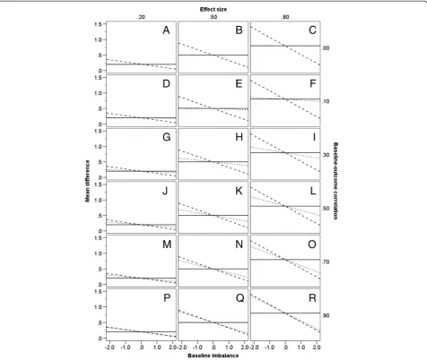
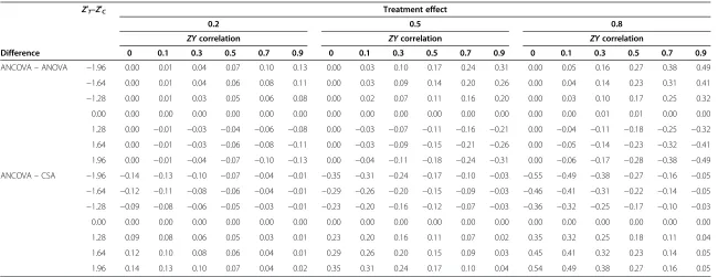
Figure 1 shows the mean estimated treatment effect and thereby the directional pattern of bias for ANOVA and CSA, in relation to ANCOVA as the reference unbiased analysis. Table 1 indicates the bias, in standardized (SD) units, for each of ANOVA and CSA, again in relation to ANCOVA. Values are given in the table conditional on the three treatment effects, the six levels ofZYcorrelation, the situation in which there is no baseline imbalance, and the six values of standardized imbalance.

The results displayed in Figure 1 demonstrate that, when there is no imbalance at baseline (i.e. Z′_T−Z′_C¼0), all three statistical methods yield the same unbiased esti-mate of treatment effect, irrespective of the level of ZY correlation or the standardized effect size. It is also clear that, for a given nominal treatment effect, the estimates yielded by ANOVA and CSA do not change in relation to the level ofZYcorrelation.

However, when treatment groups differ at baseline (i.e. Z′_T−Z′_C≠0 ) there is a noticeable difference in the estimate of treatment effect by these methods. The magnitude of this difference depends on the degree ofZYcorrelation and the size of baseline imbalance. At a given level of baseline im-balance, ANOVA and ANCOVA give precisely equivalent estimates whenZYcorrelation is zero (Figure 1 graphs A, B and C). However, the bias of ANOVA (relative to the un-biased estimates derived through ANCOVA) increases as ZYcorrelation rises and, holding ZYcorrelation constant, also increases with a higher degree of baseline imbalance. ANOVA and ANCOVA produce similar estimates of effect

when ZY correlation is less than 0.3 (see, for example,

Figure 1 graphs D, E and F), but at higherZYcorrelations, the difference in the estimate of effect for the two methods becomes more obvious (see, for example, Figure 1 graphs M, N and O). This bias is equal in magnitude for either dir-ection of imbalance. Thus, Table 1 shows there is a bias

of 0.07 SD and −0.07 SD respectively associated with

the estimate of effect by ANOVA when a standardized baseline imbalance of 1.96 exists in the same direction (i.e. Z′_T−Z′_C>0 ), or opposite direction (i.e. Z′_T−Z′_C<0 ), at a standardized treatment effect of 0.2 and aZYcorrelation of 0.5 (see Figure 1 graph J).

If the ZY correlation is large, even a small imbalance yields a substantial bias in the estimate of treatment effect when using ANOVA (for example, Figure 1 graphs N and O). Conversely, if theZYcorrelation is small, only a small bias results even if the baseline imbalance is large (for ex-ample, Figure 1 graphs H and I). Thus, from Table 1, when the ZY correlation is 0.7, ANOVA shows an upward bias with regard to ANCOVA of 0.25 SD at a standardized base-line imbalance of −1.28 and standardized treatment effect of 0.8. In contrast, when the ZY correlation is 0.3, a larger

imbalance of−1.96 produces an upward bias for ANOVA

of only 0.16 SD when estimating the same effect (Table 1). Turning to CSA, the magnitude of bias similarly is greater with an increase in the absolute value of baseline imbalance, and is equal for both directions of baseline im-balance (see, for example, Figure 1 graphs K and L). It is ap-parent from Figure 1 and Table 1 that CSA produces an opposite bias to that induced by ANOVA; when the one method overestimates the unbiased treatment effect, the other method underestimates it, and vice versa. However, in contrast to the case of ANOVA, at a given level of base-line imbalance, bias in the estimate of effect through CSA

(4)

decreases asZYcorrelation increases. When baseline imbal-ance is in the same direction as the treatment effect (i.e. Z′_T−Z′_C>0), the estimate derived from CSA is markedly

lower than that of either ANOVA or ANCOVA if ZY

correlation is low (see, for example, Figure 1 graphs F and I). Here, CSA underestimates the true treatment effect to a much larger degree than ANOVA overesti-mates it. Conversely, the bias associated with CSA is

much smaller than that of ANOVA ifZYcorrelation is

high (see, for example, Figure 1 graphs O and R). WhenZYcorrelation is at or below 0.7, CSA yields the smallest estimate of treatment effect of the three methods if baseline imbalance is in the same direction

Z′_T−Z′_C>0

as the treatment effect, and the largest esti-mate of effect if imbalance is in the opposite direction to the treatment effect Z′_T−Z′_C<0, indicating that it

provides the strongest adjustment for baseline imbalance in these circumstances. The bias of ANOVA relative to ANCOVA can be expressed algebraically by the formula:

Y′_T−Y′_C

ρ z

−2pffiffiffiffiffij jz ;

and the bias of CSA to ANCOVA by the formula:

Y′_T−Y′_C

ρ−1 z

−2pffiffiffiffiffij jz :

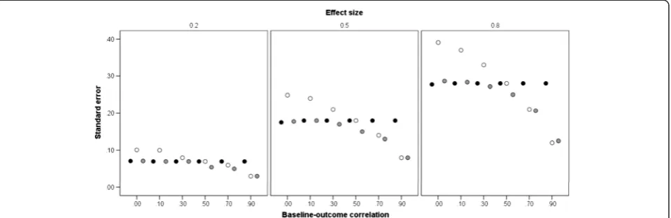
Precision

Figure 2 shows the mean standard error, at each standard-ized treatment effect size, for the three methods of analysis, at different levels of ZY correlation (the direction and Figure 1Directional bias of statistical methods.Estimates are given at differing levels of baseline-outcome correlation, treatment effect sizes, and baseline imbalance (−1.96,−1.64,−1.28, 0, 1.28, 1.64, 1.96). Estimates derived from ANCOVA represent the unbiased treatment effect. ANOVA–solid line; ANCOVA–dotted line; CSA–dashed line.

(5)

Table 1 Bias (standard deviation units) in respect of ANCOVA versus ANOVA and ANCOVA versus CSA

Difference

Z′T–Z′C Treatment effect

0.2 0.5 0.8

ZYcorrelation ZYcorrelation ZYcorrelation

0 0.1 0.3 0.5 0.7 0.9 0 0.1 0.3 0.5 0.7 0.9 0 0.1 0.3 0.5 0.7 0.9

ANCOVA–ANOVA −1.96 0.00 0.01 0.04 0.07 0.10 0.13 0.00 0.03 0.10 0.17 0.24 0.31 0.00 0.05 0.16 0.27 0.38 0.49

−1.64 0.00 0.01 0.04 0.06 0.08 0.11 0.00 0.03 0.09 0.14 0.20 0.26 0.00 0.04 0.14 0.23 0.31 0.41

−1.28 0.00 0.01 0.03 0.05 0.06 0.08 0.00 0.02 0.07 0.11 0.16 0.20 0.00 0.03 0.10 0.17 0.25 0.32

0.00 0.00 0.00 0.00 0.00 0.00 0.00 0.00 0.00 0.00 0.00 0.00 0.00 0.00 0.00 0.01 0.01 0.00 0.00

1.28 0.00 −0.01 −0.03 −0.04 −0.06 −0.08 0.00 −0.03 −0.07 −0.11 −0.16 −0.21 0.00 −0.04 −0.11 −0.18 −0.25 −0.32

1.64 0.00 −0.01 −0.03 −0.06 −0.08 −0.11 0.00 −0.03 −0.09 −0.15 −0.21 −0.26 0.00 −0.05 −0.14 −0.23 −0.32 −0.41

1.96 0.00 −0.01 −0.04 −0.07 −0.10 −0.13 0.00 −0.04 −0.11 −0.18 −0.24 −0.31 0.00 −0.06 −0.17 −0.28 −0.38 −0.49

ANCOVA–CSA −1.96 −0.14 −0.13 −0.10 −0.07 −0.04 −0.01 −0.35 −0.31 −0.24 −0.17 −0.10 −0.03 −0.55 −0.49 −0.38 −0.27 −0.16 −0.05

−1.64 −0.12 −0.11 −0.08 −0.06 −0.04 −0.01 −0.29 −0.26 −0.20 −0.15 −0.09 −0.03 −0.46 −0.41 −0.31 −0.22 −0.14 −0.05

−1.28 −0.09 −0.08 −0.06 −0.05 −0.03 −0.01 −0.23 −0.20 −0.16 −0.12 −0.07 −0.03 −0.36 −0.32 −0.25 −0.17 −0.10 −0.03

0.00 0.00 0.00 0.00 0.00 0.00 0.00 0.00 0.00 0.00 0.00 0.00 0.00 0.00 0.00 0.00 0.00 0.00 0.00

1.28 0.09 0.08 0.06 0.05 0.03 0.01 0.23 0.20 0.16 0.11 0.07 0.02 0.35 0.32 0.25 0.18 0.11 0.04

1.64 0.12 0.10 0.08 0.06 0.04 0.01 0.29 0.26 0.20 0.15 0.09 0.03 0.45 0.41 0.32 0.23 0.14 0.05

1.96 0.14 0.13 0.10 0.07 0.04 0.02 0.35 0.31 0.24 0.17 0.10 0.04 0.54 0.49 0.38 0.27 0.16 0.05

Egbewale

et

al.

BMC

Medical

Research

Methodolog

y

2014,

14

:49

Page

5

o

f

1

2

http://ww

w.biomedce

ntral.com/1

(6)

magnitude of baseline imbalance was found to have no ef-fect on precision and has therefore been ignored). The size of the standard error is proportional to the treatment effect, but this simply reflects the sample sizes corresponding to these effects. For ANOVA (black markers), the standard error is constant acrossZYcorrelations, reflecting the fact that this analysis takes no account of the baseline values. For the other two analyses, it can be observed that the standard error associated with ANCOVA (grey markers) is similar to that of ANOVA at a lowZYcorrelation, but de-creases monotonically as correlation inde-creases. Standard er-rors for CSA (white markers) are, however, variable. At a lowZYcorrelation, mean standard error is markedly higher

than that of both ANOVA and ANCOVA, whereas atZY

correlations above 0.5, it is markedly lower than that of ANOVA and comparable to that of ANCOVA. Overall, ANCOVA is the most precise analysis, especially atZY cor-relations from 0.5 to 0.9.

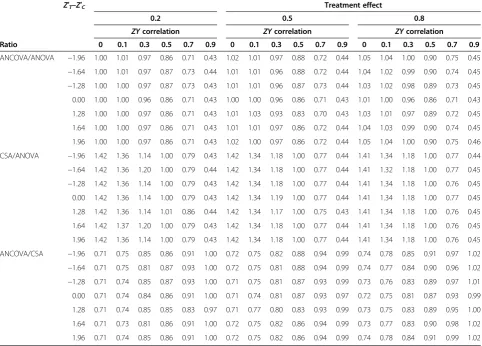
Table 2 shows the relative precision of the three analyses, expressed as a ratio of their standard errors. As in Table 1, values of these ratios are given for the three treatment ef-fects, the six levels ofZYcorrelation, the situation in which there is no baseline imbalance, and the six values of stan-dardized imbalance. Ratios greater than unity indicate that the numerator analysis has a larger standard error (i.e. is less precise) than the denominator analysis. Table 2 con-firms the equivalent precision of CSA and ANOVA at a correlation of 0.5. However, it shows that whenZY correl-ation is as low as 0.1, ANOVA can yield approximately a

36% gain in precision against CSA, whereas whenZY

cor-relation is 0.9, CSA provides approximately a 57% gain in precision over ANOVA. Table 2 also indicates that only at a correlation of 0.7 or greater does CSA produce comparable precision to that of ANCOVA.

The computed ratio of the standard errors of ANCOVA and ANOVA from the simulated datasets approximately

fits the algebraic expressionpffiffiffiffiffiffiffiffiffiffi1−ρ2_{, irrespective of whether}

or not treatment groups are balanced at baseline, and the ratios for CSA and ANOVA and for ANCOVA and CSA

approximately fit the expressions pffiffiffiffiffiffiffiffiffiffiffiffiffiffi2 1ð −ρÞ and

ffiffiffiffiffiffiffiffiffiffi 1−ρ2 ð Þ

2 1ð−ρÞ

q

; respectively.

Statistical power

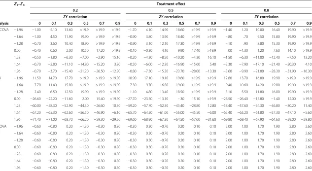
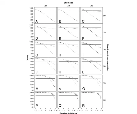
The power of ANCOVA, CSA and ANOVA is shown in Table 3 in terms of increments or decrements in relation to the nominal power of 80%, again conditional on treat-ment effect and levels ofZYcorrelation and baseline im-balance. Absolute values of power for ANCOVA, CSA and ANOVA are shown graphically in Figure 3.

The power of ANOVA is at its nominal level of 80% throughout, subject to some minor fluctuation from one simulation to the next (i.e. there are small fluctuations between the graphs in Figure 3). It is clear that for ANOVA, within any set of simulations (i.e. within any one graph in Figure 3), power is wholly unaffected by baseline imbalance, reflecting the fact that the statistical model for ANOVA has no term that represents such im-balance. It can be seen that if baseline imbalance is in the same direction as the treatment effect (indicated by

positive values of Z), the power of both ANCOVA and

CSA decreases with greater levels of imbalance, and CSA does so more markedly, especially at lower levels of ZYcorrelation. Thus, for a treatment effect of 0.2 and a

ZYcorrelation of 0.1 (Figure 3 graph D), the power of

CSA is as low as 9% if there were to be an extreme posi-tive imbalance of 1.96. Conversely, when imbalance is in the opposite direction from the treatment effect, the power of both ANCOVA and CSA exceeds the nominal

80% power of ANOVA, and if ZYcorrelation is 0.7 or

greater in these circumstances (Figure 3 graphs M to R), the superiority of ANCOVA and CSA is equivalent. If, Figure 2Standard errors of statistical methods.Estimates are given at differing levels of baseline-outcome correlation, conditional on treatment effect. The markers show the mean standard error, averaged across the treatment effects. ANOVA–black markers; ANCOVA–grey markers; CSA–white markers.

(7)

however, ZY correlation is 0.3 or less in these circum-stances, the power of CSA exceeds that of ANCOVA when negative baseline imbalance is most extreme (Fig-ure 3 graphs D to I). If there is no baseline imbalance, the power of ANCOVA is either greater than or equal to that of ANOVA, whereas the power of CSA is superior to that of ANOVA at high correlations but inferior at

low correlations. WhenZYcorrelation is zero, ANCOVA

has power approximately equivalent to that of ANOVA (Figure 3 graphs A to C).

Discussion

This simulation study has examined the effect of baseline imbalance in an RCT on the bias and precision of estimates of treatment effect, and the power of a statistical test condi-tional on such imbalance. Although the statistical implica-tions of baseline imbalance have previously been described, they have not hitherto been simultaneously quantified for these three analyses in relation to various combinations of levels of associated trial characteristics: effect size, degree of baseline-outcome (ZY)correlation and both magnitude and direction of baseline imbalance.

ANCOVA is known to produce unbiased estimates of treatment effect in the presence of baseline imbalance when groups are randomized [19,20]. ANOVA and CSA, how-ever, produce biased estimates in such circumstances. For both ANOVA and CSA, the direction of bias is related to the direction of baseline imbalance, and bias is greatest when baseline imbalance, in either direction, is most

pro-nounced. At a low ZYcorrelation, ANOVA exhibits less

bias than CSA, but at a highZYcorrelation the reverse is the case. In a situation in which ANOVA overestimates the unbiased treatment effect, CSA underestimates it, and vice versa. Both ANOVA and CSA show equal levels of bias (al-beit in different directions) when theZYcorrelation is 0.5.

When ZYcorrelation is 0, estimates from ANCOVA and

ANOVA are equivalent, as the absence of correlation means that the ANCOVA takes no account of imbalance and thereby reduces to ANOVA.

As regards precision, ANOVA and CSA yield less pre-cise estimates than ANCOVA. ANOVA is progressively

less precise than ANCOVA as ZYcorrelation increases;

by contrast, CSA shows increasing precision as ZY

cor-relation increases. CSA is less precise than ANOVA at

Table 2 Design effect (ratio of standard errors) in respect of ANCOVA versus ANOVA, CSA versus ANOVA, and ANCOVA versus CSA

Ratio

0.2 0.5 0.8

0 0.1 0.3 0.5 0.7 0.9 0 0.1 0.3 0.5 0.7 0.9 0 0.1 0.3 0.5 0.7 0.9

ANCOVA/ANOVA −1.96 1.00 1.01 0.97 0.86 0.71 0.43 1.02 1.01 0.97 0.88 0.72 0.44 1.05 1.04 1.00 0.90 0.75 0.45 −1.64 1.00 1.01 0.97 0.87 0.73 0.44 1.01 1.01 0.96 0.88 0.72 0.44 1.04 1.02 0.99 0.90 0.74 0.45 −1.28 1.00 1.00 0.97 0.87 0.73 0.43 1.01 1.01 0.96 0.87 0.73 0.44 1.03 1.02 0.98 0.89 0.73 0.45 0.00 1.00 1.00 0.96 0.86 0.71 0.43 1.00 1.00 0.96 0.86 0.71 0.43 1.01 1.00 0.96 0.86 0.71 0.43

1.28 1.00 1.00 0.97 0.86 0.71 0.43 1.01 1.03 0.93 0.83 0.70 0.43 1.03 1.01 0.97 0.89 0.72 0.45

1.64 1.00 1.00 0.97 0.86 0.71 0.43 1.01 1.01 0.97 0.86 0.72 0.44 1.04 1.03 0.99 0.90 0.74 0.45

1.96 1.00 1.00 0.97 0.86 0.71 0.43 1.02 1.00 0.97 0.86 0.72 0.44 1.05 1.04 1.00 0.90 0.75 0.46

CSA/ANOVA ₋1.96 1.42 1.36 1.14 1.00 0.79 0.43 1.42 1.34 1.18 1.00 0.77 0.44 1.41 1.34 1.18 1.00 0.77 0.44 −1.64 1.42 1.36 1.20 1.00 0.79 0.44 1.42 1.34 1.18 1.00 0.77 0.44 1.41 1.32 1.18 1.00 0.77 0.45 −1.28 1.42 1.36 1.14 1.00 0.79 0.43 1.42 1.34 1.18 1.00 0.77 0.44 1.41 1.34 1.18 1.00 0.76 0.45 0.00 1.42 1.36 1.14 1.00 0.79 0.43 1.42 1.34 1.19 1.00 0.77 0.44 1.41 1.34 1.18 1.00 0.77 0.45

1.28 1.42 1.36 1.14 1.01 0.86 0.44 1.42 1.34 1.17 1.00 0.75 0.43 1.41 1.34 1.18 1.00 0.76 0.45

1.64 1.42 1.37 1.20 1.00 0.79 0.43 1.42 1.34 1.18 1.00 0.77 0.44 1.41 1.34 1.18 1.00 0.76 0.45

1.96 1.42 1.36 1.14 1.00 0.79 0.43 1.42 1.34 1.18 1.00 0.77 0.44 1.41 1.34 1.18 1.00 0.76 0.45

ANCOVA/CSA −1.96 0.71 0.75 0.85 0.86 0.91 1.00 0.72 0.75 0.82 0.88 0.94 0.99 0.74 0.78 0.85 0.91 0.97 1.02 −1.64 0.71 0.75 0.81 0.87 0.93 1.00 0.72 0.75 0.81 0.88 0.94 0.99 0.74 0.77 0.84 0.90 0.96 1.02 −1.28 0.71 0.74 0.85 0.87 0.93 1.00 0.71 0.75 0.81 0.87 0.93 0.99 0.73 0.76 0.83 0.89 0.97 1.01 0.00 0.71 0.74 0.84 0.86 0.91 1.00 0.71 0.74 0.81 0.87 0.93 0.97 0.72 0.75 0.81 0.87 0.93 0.99

1.28 0.71 0.74 0.85 0.85 0.83 0.97 0.71 0.77 0.80 0.83 0.93 0.99 0.73 0.75 0.83 0.89 0.95 1.00

1.64 0.71 0.73 0.81 0.86 0.91 1.00 0.72 0.75 0.82 0.86 0.94 0.99 0.73 0.77 0.83 0.90 0.98 1.02

1.96 0.71 0.74 0.85 0.86 0.91 1.00 0.72 0.75 0.82 0.86 0.94 0.99 0.74 0.78 0.84 0.91 0.99 1.02

(8)

Table 3 Increments (positive values) and decrements (negative values) of power (%) for ANCOVA, ANOVA and CSA relative to a nominal power of 80% and conditional upon levels of baseline imbalance andZYcorrelation

0.2 0.5 0.8

Analysis 0 0.1 0.3 0.5 0.7 0.9 0 0.1 0.3 0.5 0.7 0.9 0 0.1 0.3 0.5 0.7 0.9

ANCOVA −1.96 −1.00 5.10 13.60 >19.9 >19.9 >19.9 −1.70 4.10 14.90 18.60 >19.9 >19.9 −1.40 1.20 10.00 16.40 19.90 >19.9

−1.64 −1.00 4.50 11.90 19.90 >19.9 >19.9 −0.90 3.80 13.90 18.40 >19.9 >19.9 –.80 .70 9.50 15.80 19.90 >19.9

−1.28 −0.70 3.60 10.40 18.90 >19.9 >19.9 −0.90 3.10 12.10 17.30 >19.9 >19.9 –.10 .90 8.80 15.30 19.90 >19.9

0.00 −0.40 0.60 2.00 10.50 17.20 >19.9 −0.10 −0.30 4.10 9.90 17.40 >19.9 .00 −1.30 1.20 7.60 14.10 >19.9

1.28 −0.50 −1.80 −6.30 −7.00 −2.90 15.10 −0.20 −4.30 −8.50 −10.20 −4.30 16.10 −1.50 −6.30 −11.00 −12.40 −7.50 13.20

1.64 −0.70 −2.80 −11.10 −14.80 −15.20 3.80 −0.50 −6.00 −12.30 −16.90 −15.60 5.40 −2.30 −7.90 −17.10 −21.40 −20.30 4.10

1.96 −0.70 −3.70 −15.40 −21.20 −26.50 −12.90 −0.80 −7.30 −15.30 −23.70 −28.00 −13.30 −3.60 −9.90 −21.00 −28.30 −31.90 −16.30

CSA −1.96 11.50 14.70 17.70 >19.9 >19.9 >19.90 10.90 17.10 19.10 19.60 >19.9 >19.9 12.80 13.70 16.00 19.90 >19.9 >19.9

−1.64 7.70 11.40 15.80 >19.9 >19.9 >19.90 7.30 9.70 16.80 19.00 >19.9 >19.9 9.40 10.60 14.20 19.80 19.90 >19.9

−1.28 2.40 6.50 12.50 19.90 >19.9 >19.90 1.10 4.80 13.40 18.50 >19.9 >19.9 3.10 5.50 11.80 16.00 19.90 >19.9

0.00 −26.60 −22.20 −11.60 2.00 15.40 >19.90 −27.70 −23.50 −13.10 –.30 15.10 >19.9 −28.50 −26.40 −15.80 −1.40 12.00 >19.9

1.28 −60.00 −58.30 −52.90 −44.30 −26.60 10.30 −59.20 −57.70 −52.30 −45.40 −28.80 12.80 −58.40 −57.60 −54.30 −46.80 −30.20 11.40

1.64 −67.20 −65.30 −62.60 −56.50 −46.90 −6.10 −65.70 −64.50 −61.00 −56.00 −45.50 −6.00 −65.40 −65.20 −61.80 −57.30 −47.10 −5.60

1.96 −71.40 −71.00 −68.70 −66.20 −59.30 −29.50 −69.60 −68.90 −67.30 −64.50 −57.60 −31.60 −69.80 −69.40 −67.90 −64.60 −59.00 −29.80

ANOVA −1.96 −0.60 −0.80 0.20 −1.30 −0.30 0.80 −0.30 0.30 −0.70 0.20 0.10 0.10 2.00 1.00 1.70 1.90 2.80 2.60

−1.64 −0.60 −0.80 0.20 −1.30 −0.30 0.80 −0.30 0.30 −0.70 0.20 0.10 0.10 2.00 1.00 1.70 1.90 2.80 2.60

−1.28 −0.60 −0.80 0.20 −1.30 −0.30 0.80 −0.30 0.30 −0.70 0.20 0.10 0.10 2.00 1.00 1.70 1.90 2.80 2.60

0.00 −0.60 −0.80 0.20 −1.30 −0.30 0.80 −0.30 0.30 −0.70 0.20 0.10 0.10 2.00 1.00 1.70 1.90 2.80 2.60

1.28 −0.60 −0.80 0.20 −1.30 −0.30 0.80 −0.30 0.30 −0.70 0.20 0.10 0.10 2.00 1.00 1.70 1.90 2.80 2.60

1.64 −0.60 −0.80 0.20 −1.30 −0.30 0.80 −0.30 0.30 −0.70 0.20 0.10 0.10 2.00 1.00 1.70 1.90 2.80 2.60

1.96 −0.60 −0.80 0.20 −1.30 −0.30 0.80 −0.30 0.30 −0.70 0.20 0.10 0.10 2.00 1.00 1.70 1.90 2.80 2.60

Maximum increment is given as >19.9 since this would represent a conditional power in excess of 99.9%. Increments/decrements in power for ANOVA are due to random variation of the simulated dataset around the nominal 80% power.

Egbewale

et

al.

BMC

Medical

Research

Methodolog

y

2014,

14

:49

Page

8

o

f

1

2

http://ww

w.biomedce

ntral.com/1

(9)

ZYcorrelations below 0.5, but more precise atZY corre-lations greater than 0.5, and both analyses present the same magnitude of associated standard error when the correlation is 0.5. In no situation do either CSA or ANOVA exceed the precision of ANCOVA.

The results for statistical power of the three analyses are not straightforward. The greater precision noted for ANCOVA might suggest that it would be uncondition-ally the most powerful analysis. Yet, as Figure 3 shows, whilst under some circumstances its power exceeds the nominal 80% power of ANOVA, under other circum-stances ANOVA has greater power. This can be ex-plained by the adjusted treatment effect derived through ANCOVA. When baseline imbalance is in the opposite direction from the treatment effect, ANCOVA corrects the resulting bias by producing an adjusted treatment ef-fect that is larger than the nominal treatment efef-fect, and

ANCOVA therefore has greater power to detect this effect than ANOVA has to detect the nominal effect, at the same sample size. Correspondingly, when imbalance is in the same direction as the treatment effect, ANCOVA corrects the bias by adjusting the treatment ef-fect downwards; its power to detect this efef-fect is therefore less than that of ANOVA to detect the nominal treatment effect. However, whenZYcorrelation is 0 (Figure 3 graphs A to C), ANCOVA and ANOVA produce equivalent estimates of treatment effect, as noted earlier, and the difference in power therefore essentially disappears. This phenomenon also explains why baseline imbalance affects precision and power differently; precision is unaffected by imbalance but power reflects imbalance when it is calcu-lated in relation to an adjusted treatment effect. When there is no imbalance, the adjusted treatment effect equals the nominal treatment effect and here ANCOVA is more Figure 3Power (%) of statistical methods.Estimates are given at differing levels of baseline-outcome correlation, treatment effect sizes, and baseline imbalance (−1.96,−1.64,−1.28, 0, 1.28, 1.64, 1.96). ANOVA–solid line; ANCOVA–dotted line; CSA–dashed line.

(10)

powerful than ANOVA by virtue of its greater precision [18,31,32]. An important point to emphasize is that, in the presence of imbalance, nominal power is inappropriate due to the underlying bias in the estimation of the true treat-ment effect by ANOVA, which fails to address the baseline imbalance of the two treatment groups. As regards the ana-lyses that accommodate baseline imbalance, ANCOVA is unconditionally more powerful than CSA, especially at lowerZYcorrelations [33].

The power of CSA shows a similar pattern to that of ANCOVA when ZY correlation is 0.7 or greater. At lower correlations, however, it demonstrates greater extremes of

power than ANCOVA –higher than ANCOVA with

im-balance in the opposite direction from the treatment effect and lower than ANCOVA with imbalance in the same dir-ection. This indicates CSA’s over-correction of bias, in both directions, whenZYcorrelation is low; this stems from its failure to account for regression to the mean [24,34]. In the absence of imbalance, the power of CSA exceeds the

nom-inal 80% power of ANOVA when ZYcorrelation is high,

but is lower than that of ANOVA when ZYcorrelation is

low. This reflects the relative precision of these two ana-lyses conditional uponZYcorrelation; CSA is the more pre-cise at high correlations whereas ANOVA is the more precise a low correlations, as indicated by the ratios of standard errors in Table 2.

Relative to ANCOVA, the alternative analyses are thus li-able to be either too conservative or too liberal [26]. It is clear therefore that the use of either ANOVA or CSA is in-advisable when baseline imbalance exists. Although all three methods are unbiased when there is no baseline im-balance, the likelihood is that in a clinical trial with several baseline covariates there will be some degree of imbalance across a number, if not all, of these variables. Similarly, the level of correlation between these covariates and the out-come variable is likely to be greater than zero (or possibly less than zero, though baseline values of the outcome vari-able are more likely to be positively than negatively corre-lated with post-treatment values). Moreover, ANCOVA is consistently the most precise method of analysis and hence delivers greatest efficiency in respect of testing against the null hypothesis and reducing the type II error. Our results concur with previous literature that emphasizes the advan-tages of covariate adjustment [3,8,9,12-16,24,35].

These simulations are based on imbalance in a single covariate. Where imbalance exists in a number of covar-iates, the degree of bias associated with either ANOVA or CSA will depend upon the combined effect of imbal-ances that may be in different directions, and upon the particular ZYcorrelations associated with each of these covariates. However, loss of precision (and hence of stat-istical power) through the use of ANOVA or CSA is likely to be greater with imbalance in multiple covariates than with imbalance in a single covariate, as there will

normally be a greater proportion of variance in the out-come measure that is unaccounted for by either of these analyses.

Our results show the advantages of ANCOVA in redu-cing bias, increasing precision and providing appropriate power of statistical testing across a number of practical sit-uations commonly seen in clinical trials. Several authors [2,34,36-39] argue that covariates should be selected a priori in terms of their prognostic importance, rather than on the basis of examining baseline imbalance in the trial

data – even large imbalance is of little consequence in

terms of bias if the covariate is not related to outcome. Moreover, the primary analysis in an RCT should be pre-specified [40,41]. Accordingly, our findings suggest that ANCOVA should be adopted as the analysis of choice, regardless of the magnitude of imbalance observed in the trial data. Consideration should also be given to achieving balance in important prognostic covariates at baseline in addition to subsequent statistical adjustment [42] – e.g. through stratified randomization or covariate-adaptive methods of allocation [11,43,44].

Limitations

The conditions under which we have investigated the effect

of baseline imbalance – in terms of magnitude of effect

sizes, baseline imbalance andZYcorrelation–are plausible and realistic, although the extremes of baseline imbalance examined will, reassuringly, be uncommon. Our findings are therefore readily transferable to specific real-life RCT scenarios. However, our findings assume equal allocation, and results may differ where this is not the case. Nor do our findings necessary generalize fully to trials where groups are not formed by randomization [45] or where out-comes are binary or time-to-event [28,42,46]. These results are also based on analyses whose assumptions were opti-mally satisfied through the simulation process, and are likely to differ in respect of real-life data that depart from such assumptions–e.g. a skewed outcome variable, or

het-erogeneous ZY regression coefficients between groups.

Large trials will produce data that are robust to certain de-viations in the assumptions underlying parametric analysis. Nonetheless, future work could usefully explore the impact of some of these deviations on the conclusions of the current study.

Conclusion

In conclusion, ANCOVA should be the analysis of choice, a priori, for RCTs with a single post-treatment outcome measure previously measured at baseline; its superiority is particularly marked when baseline imbalance is present,

but also – in terms of precision – when groups are

bal-anced at baseline. We specifically caution against the use of ANOVA when the baseline-outcome correlation is (or is anticipated to be) moderate-to-large, and against CSA

(11)

when it is (or is anticipated to be) small-to-moderate. Randomization generally leads to well-balanced groups, though non-systematic differences often arise across a number of covariates, and hence adjustment through ANCOVA is recommended to reduce risk of bias whilst also improving the precision of estimates and the power of the statistical test.

Appendix

Simulation program in STATA. The prime identifies values that are specific to a particular simulation; i.e. r′indicates r = 0.1, r = 0.3, r = 0.5, r = 0.7, r = 0.9; y′ indicates y = 0.2, y = 0.5, y = 0.8; z′ indicates standardized imbalance (the standard error of absolute imbalance multiplied by the ap-propriate standard normal deviate).

set seed set obs n

[defines number of observations (n) for the trial] g g = mod(_n,2)

[defines two treatment groups – Control (0); Treat-ment(1)]

g z = invnorm(uniform())*1

[generates normally distributed baseline scores (z) with mean = 0 and SD = 1 and randomly assigns these to treatment groups]

g r = r′

[generates a predetermined correlation between base-line and post-treatment scores]

g k = invnorm(uniform())*1

[generates another normally distributed set of scores (k)] g y = z*r + k*(1−r^2)^.5

[transforms k into an outcome score (y) that has a pre-determined correlation with the baseline score (z)]

replace z = z + g*z′

[applies a predetermined direction-specific baseline im-balance to the treatment groups; with ‘z + g’, imbalance is in the same direction as the treatment effect, but with

‘z−g’it is in the opposite direction] replace y = y + g*y′

[creates a predetermined treatment effect] g c = y−z

[generates change scores for the treatment groups] regress y g

[performs analysis of variance] regress c g

[performs change-score analysis] regress y g z

[performs analysis of covariance]

Abbreviations

ANCOVA:Analysis of covariance; ANOVA: Analysis of variance; CSA: Change-score analysis; RCT: Randomized controlled trial.

Competing interests

The authors have no competing interests.

Authors’contributions

JS and ML conceived the study. All authors designed the study. BEE planned and performed the simulations. All authors interpreted the data. All authors drafted the manuscript and approved the final version.

Acknowledgments

The authors wish to thank Peter Jones for helpful advice on the study.

Received: 30 November 2013 Accepted: 31 March 2014 Published: 9 April 2014

References

1. Rosenberger WF, Lachin JM:Randomization in Clinical Trials: Theory and Practice.New York, NY: Wiley-Interscience; 2002.

2. Roberts C, Torgerson DJ:Baseline imbalance in randomised controlled trials.BMJ1999,319:185.

3. Altman DG, Doré CJ:Baseline comparisons in randomized clinical trials.

Stat Med1991,10:797–799.

4. Tu D, Shalay K, Pater J:Adjustment of treatment effect for covariates in clinical trials: statistical and regulatory issues.Drug Inf J2000,34:511–523. 5. Ciolino JD, Martin RH, Zhao W, Jauch EC, Hill MD, Palesch YY:Covariate

imbalance and adjustment for logistic regression analysis of clinical trial data.J Biopharm Stat2013,23:1383–1402.

6. Piantadosi S:Clinical Trials: a Methodologic Perspective.2nd edition. New York: Wiley; 2005.

7. Kernan WN, Makuch RM:Response.J Clin Epidemiol2001,54:105. 8. Scott NW, McPherson GC, Ramsay CR, Campbell MK:The method of

minimization for allocation to clinical trials: a review.Control Clin Trials

2002,23:662–674.

9. Hagino A, Hamada C, Yoshimura I, Ohashi Y, Sakamoto J, Nakazato H: Statistical comparison of random allocation methods in cancer clinical trials.Control Clin Trials2004,25:572–584.

10. Taves DR:Faulty assumptions in Atkinson’s criteria for clinical trial design.

J R Stat Soc2004,167:179–181.

11. Rosenberger WF, Sverdlov O:Handling covariates in the design of clinical trials.Stat Sci2008,23:404–419.

12. Frison L, Pocock SJ:Repeated measures in clinical trials: analysis using mean summary statistics and its implications for design.Stat Med1992, 11:1685–1704.

13. Hernández AV, Eijkemans MJ, Steyerberg EW:Randomized controlled trials with time-to-event outcomes: how much does prespecified covariate adjustment increase power?Ann Epidemiol2006,16:41–48.

14. Van Breukelen GJP:ANCOVA versus change from baseline had more power in randomized studies and more bias in nonrandomized studies.

J Clin Epidemiol2006,59:920–925.

15. Kent DM, Trikalinos TA, Hill MD:Are unadjusted analyses of clinical trials inappropriately biased toward the null?Stroke2009,40:672–673. 16. Ciolino JD, Martin RH, Zhao W, Hill MD, Jauch EC, Palesch YY:Measuring

continuous baseline covariate imbalances in clinical trial data.

Stat Methods Med Res2011, doi:10.1177/0962280211416038. 17. Austin PC, Manca A, Zwarenstein M, Juurlink DN, Stanbrook MB:A

substantial and confusing variation exists in handling of baseline covariates in randomized controlled trials: a review of trials published in leading medical journals.J Clin Epidemiol2010,63:142–153.

18. Vickers AJ:The use of percentage change from baseline as an outcome in a controlled trial is statistically inefficient: a simulation study.BMC Med Res Methodol2001,1:6.

19. Matthews JNS:Introduction to Randomized Controlled Clinical Trials.2nd edition. Boca Raton, FL: Chapman & Hall/CRC; 2006.

20. Huitema B:The Analysis of Covariance and Alternatives: Statistical Methods for Experiments, Quasi-Experiments, and Single-Case Studies.2nd edition. Hoboken, NJ: Wiley; 2011.

21. Christensen E, Neuberger J, Crowe J, Altman DG, Popper H, Portmann B, Doniach D, Ranek L, Tygstrup N, Williams R:Beneficial effect of azathioprine and prediction of prognosis in primary biliary cirrhosis. Final results of an international trial.Gastroenterology1985,89:1084–1091. 22. Beach ML, Meier P:Choosing covariates in the analysis of clinical trials.

Control Clin Trials1989,10(4 Suppl):161S–175S.

(12)

23. Steyerberg EW, Bossuyt PMM, Lee KL:Clinical trials in acute myocardial infarction: should we adjust for baseline characteristics?Am Heart J2000, 139:745–751.

24. Vickers AJ, Altman DG:Analysing controlled trials with baseline and follow up measurements.BMJ2001,323:1123–1124.

25. Senn SJ:Baseline comparisons in randomised clinical trials.Stat Med

1991,10:1157–1160.

26. Overall JE, Magee KN:Directional baseline differences and Type I error probabilities in randomized clinical trials.J Biopharm Stat1992,2:189–203. 27. Overall JE, Doyle SR:Implications of chance baseline differences in

repeated measurement designs.J Biopharm Stat1994,4:199–216. 28. Chu R, Walter SD, Guyatt G, Devereaux PJ, Walsh M, Thorlund K, Thabane L:

Assessment and implication of prognostic imbalance in randomized controlled trials with a binary outcome–a simulation study.PLoS One

2012,7:e36677.

29. Pocock SJ, Assmann SE, Enos LE, Kasten LE:Subgroup analysis, covariate adjustment and baseline comparisons in clinical trial reporting: current practice and problems.Stat Med2002,21:2917–2930.

30. Cohen J:Statistical Power Analysis for the Behavioral Sciences.2nd edition. Hillsdale NJ: Lawrence Erlbaum; 1988.

31. Tu YK, Blance A, Clerehugh V, Gilthorpe MS:Statistical power for analyses of changes in randomized controlled trials.J Dent Res2005,84:283–287. 32. Wei L, Zhang J:Analysis of data with imbalance in the baseline outcome

variable for randomized clinical trials.Drug Inf J2001,35:1201–1214. 33. Egger MJ, Coleman ML, Ward JR, Reading JC, Williams HJ:Uses and abuses

of analysis of covariance in clinical trials.Control Clin Trials1985,6:12–24. 34. Twisk J, Proper K:Evaluation of the result of a randomized controlled

trial: how to define changes between baseline and follow up.

J Clin Epidemiol2004,57:223–228.

35. Assmann SF, Pocock SJ, Enos LE, Kasten LE:Subgroup analysis and other (mis)uses of baseline data in clinical trials.Lancet2000,355:1064–1069. 36. Armitage P, Gehan EA:Statistical methods for the identification and use

of prognostic factors.Int J Cancer1974,13:16–36.

37. Senn SJ:Covariate imbalance and random allocation in clinical trials.

Stat Med1989,8:467–475.

38. Senn SJ:Testing for baseline balance in clinical trials.Stat Med1994, 13:1715–1726.

39. Raab GM, Day S, Sales J:How to select covariates to include in the analysis of a clinical trial.Control Clin Trials2000,21:330–342. 40. DHHS:Guidance for Industry E9: Statistical Principles for Clinical Trials.

Rockville MD: Department of Health and Human Services; 1998.

41. Chan A-W, Tetzlaff JM, Gøtzsche PC, Altman DG, Mann H, Berlin JA, Dickersin K, Hróbjartsson A, Schulz KF, Parulekar WR, Krleža-Jeric K, Laupacis A, Moher D:SPIRIT 2013 explanation and elaboration: guidance for protocols of clinical trials.BMJ2013,346:e7586.

42. Ciolino J, Zhao W, Martin R, Palesch Y:Quantifying the cost in power of ignoring continuous covariates imbalances in clinical trial randomization.

Contemp Clin Trials2011,32:250–259.

43. Kernan WN, Viscoli CM, Makuch RW, Brass LM, Horwitz RI:Stratified randomization for clinical trials.J Clin Epidemiol1999,52:19–26. 44. Kahan BC, Morris TP:Reporting and analysis of trials using stratified

randomisation in leading medical journals: review and reanalysis.

BMJ2012,345:e5840.

45. Overall JE, Ashby B:Baseline corrections in experimental and quasi-experimental clinical trials.Neuropsychopharmacology1991, 4:273–281.

46. Hernández AV, Steyerberg EW, Habbema JD:Covariate adjustment in randomized controlled trials with dichotomous outcomes increases statistical power and reduces sample size requirements.J Clin Epidemiol

2004,57:454–460.

doi:10.1186/1471-2288-14-49

Cite this article as:Egbewaleet al.:Bias, precision and statistical power of analysis of covariance in the analysis of randomized trials with baseline imbalance: a simulation study.BMC Medical Research Methodology201414:49.

Submit your next manuscript to BioMed Central and take full advantage of:

• Convenient online submission

• Thorough peer review

• No space constraints or color ﬁgure charges

• Immediate publication on acceptance

• Inclusion in PubMed, CAS, Scopus and Google Scholar

• Research which is freely available for redistribution

Submit your manuscript at www.biomedcentral.com/submit