Collective Matrix Completion
Mokhtar Z. Alaya [email protected]
Modal’X, UPL, Univ Paris Nanterre, F92000 Nanterre France
Olga Klopp [email protected]
ESSEC Business School and CREST, F95021 Cergy France
Editor:Xiaotong Shen
Abstract
Matrix completion aims to reconstruct a data matrix based on observations of a small number of its entries. Usually in matrix completion a single matrix is considered, which can be, for example, a rating matrix in recommendation system. However, in practical situations, data is often obtained from multiple sources which results in a collection of matrices rather than a single one. In this work, we consider the problem of collective matrix completion with multiple and heterogeneous matrices, which can be count, binary, continuous, etc. We first investigate the setting where, for each source, the matrix entries are sampled from an exponential family distribution. Then, we relax the assumption of exponential family distribution for the noise. In this setting, we do not assume any specific model for the observations. The estimation procedures are based on minimizing the sum of a goodness-of-fit term and the nuclear norm penalization of the whole collective matrix. We prove that the proposed estimators achieve fast rates of convergence under the two considered settings and we corroborate our results with numerical experiments.
Keywords: High-dimensional prediction; Exponential families; Low-rank matrix estima-tion; Nuclear norm minimizaestima-tion; Low-rank optimizaestima-tion;
1. Introduction
Completing large-scale matrices has recently attracted great interest in machine learning and data mining since it appears in a wide spectrum of applications such as recommender systems (Koren et al., 2009; Bobadilla et al., 2013), collaborative filtering (Netflix chal-lenge) (Goldberg et al., 1992; Rennie and Srebro, 2005), sensor network localization (So and Ye, 2005; Drineas et al., 2006; Oh et al., 2010), system identification (Liu and Vanden-berghe, 2009), image processing (Hu et al., 2013), among many others. The basic principle of matrix completion consists in recovering all the entries of an unknown data matrix from incomplete and noisy observations of its entries.
To address the high-dimensionality in matrix completion problem, statistical inference based on low-rank constraint is now an ubiquitous technique for recovering the underlying data matrix. Thus, matrix completion can be formulated as minimizing the rank of the matrix given a random sample of its entries. However, this rank minimization problem is in general NP-hard due to the combinatorial nature of the rank function (Fazel et al., 2001; Fazel, 2002). To alleviate this problem and make it tractable, convex relaxation strategies
c
were proposed, e.g., the nuclear norm relaxation (Srebro et al., 2005; Candes and Tao, 2010; Recht et al., 2010; Negahban and Wainwright, 2011; Klopp, 2014) or the max-norm relaxation (Cai and Zhou, 2016). Among those surrogate approximations, nuclear norm, which is defined as the sum of the singular values of the matrix or the `1-norm of its spectrum, is probably the most widely used penalty for low-rank matrix estimation, since it is the tightest convex lower bound of the rank (Fazel et al., 2001).
Motivations. Classical matrix completion focus on a single matrix, whereas in practical situations data is often obtained from a collection of matrices that may cover multiple and heterogeneous sources. For example, in e-commerce users express their feedback for different items such as books, movies, music, etc. In social networks like Facebook and Twitter users often share their opinions and interests on a variety of topics (politics, social events, health). In this examples, informations from multiple sources can be viewed as a collection of matrices coupled through a common set of users.
Rather than exploiting user preference data from each source independently, it may be beneficial to leverage all the available user data provided by various sources in order to generate more encompassing user models (Cantador et al., 2015). For instance, some recommender system runs into the so-called cold-start problem(Lam et al., 2008). A user is new or “cold” in a source when he has few to none rated items. Such user may have a rating history in auxiliary sources and we can use his profile in the auxiliary sources to recommend relevant items in the target source. For example, a user’s favorite movie genres may be derived from his favorite book genres. Therefore, this shared structure among the sources can be useful to get better predictions (Singh and Gordon, 2008; Bouchard et al., 2013; Gunasekar et al., 2016).
More generally speaking, collective matrix completion finds a natural application in the problem of recommender system with side information. In this problem, in addition to the conventional user-item matrix, it is assumed that we have side information about each user (Chiang et al., 2015; Jain and Dhillon, 2013; Fithian and Mazumder, 2018; Agarwal et al., 2011). For example, in blog recommendation task, we may have access to user generated content (images, tags and text) or user activity (e.g., likes and reblogs). Such side information may be used to improve the quality of recommendation of blogs of interest (Shin and Lee, 2015).
Based on the type of available side information, various methods for recommender sys-tems with side information have been proposed. It can be user generated content (Armen-tano et al., 2013; Hannon et al., 2010), user/item profile or attribute (Agarwal et al., 2011), social network (Jamali and Ester, 2010; Ma et al., 2011) and context information (Natara-jan et al., 2013). A very interesting surveys of the state-of-the-art methods can be found in (Fithian and Mazumder, 2018; Natarajan et al., 2013).
Main contributions and related literature. In this paper, we extend the theory of low-rank matrix completion to a collection of multiple and heterogeneous matrices. We first consider general matrix completion setting where we assume that for each matrix its entries are sampled from natural exponential distributions (Lehmann and Casella, 1998). In this setting, we may have Gaussian distribution for continuous data; Bernoulli for binary data; Poisson for count-data, etc. In a second part, we relax the assumption of exponential family distribution for the noise and we do not assume any specific model for the observations. This approach is more popular and widely used in machine learning. The proposed estimation procedure is based on minimizing the sum of a goodness-of-fit term and the nuclear norm penalization of the whole collective matrix. The key challenge in our analysis is to use joint low-rank structure and our algorithm is far from the trivial one which consists in estimating each source matrix separately. We provide theoretical guarantees on our estimation method and show that the collective approach provides faster rate of convergences. We further corroborate our theoretical findings through simulated experiments.
Previous works on collective matrix completion are mainly based on matrix factoriza-tion (Srebro et al., 2005). In a nutshell, this approach fits the target matrix as the product of two low-rank matrices. Matrix factorization gives rise to non-convex optimization prob-lems and its theoretical understanding is quite limited. For example, Singh and Gordon (2008) proposed the collective matrix factorization that jointly factorizes multiple matri-ces sharing latent factors. As in our setting, each matrix can have a different value type and error distribution. In Singh and Gordon (2008), the authors use Bregman divergences to measure the error and extend standard alternating projection algorithms to this set-ting. They consider a quite general setting which includes as a particular case the nuclear norm penalization approach that we study in the present paper. They do not provide any theoretical guarantee. A Bayesian model for collective matrix factorization was proposed in Singh and Gordon (2010). Horii et al. (2014) and Xu et al. (2016) also consider collective matrix factorization and investigate the strength of the relation among the source matri-ces. Their estimation procedure is based on penalization by the sum of the nuclear norms of the sources. The convex formulation for collective matrix factorization was proposed in Bouchard et al. (2013) where the authors consider a general situation when the set of matrices do not necessarily have a common set of rows/columns. When this is the case, the estimator proposed in Bouchard et al. (2013) is quite similar to ours. Their algorithm is based on the iterative Singular Value Thresholding and the authors conduct empirical evaluations of this approach on two real data sets.
systems. The theoretical analysis in the present paper is carried out for general sampling distributions.
Similar to our setting, matrix completion with side information explores the available user data provided by various sources. For instance Jain and Dhillon (2013) and Xu et al. (2013) introduce the so-called Inductive Matrix Completion (IMC). It models side informa-tion as knowledge of feature spaces. They show that if the features are perfect (e.,g., see Definition 1 in Chiang et al. (2018) for perfect side information), the sample complexity can be reduced. More precisely, in works on matrix completion with side information, it is usually assumed that one has partially observed low-rank matrix of interest M ∈ Rd1×d2
and, additionally, one has access to two matrices of features A ∈ Rd1×r1 and B ∈ Rd2×r2
where each row of A (or B) denotes the feature of thei-th row (or column) entity of M, ri < di fori= 1,2 andM =AZBT . The main difference with our setting is that, here,A
and B are assumed to be fully observed while our model allows also missing observations for the set of features. The perfect side information assumption is strong and hard to meet in practice. Chiang et al. (2015) relaxed it by assuming that the side information may be noisy (not perfect). In this approach, referred as DirtyIMC, they assume that the unknown matrix is modeled asM =AZBT+N where the residual matrixN models imperfections and noise in the features.
Several works consider matrix completion with side information. For example, Chiang et al. (2015) proposes a method based on penalization by the sum of the nuclear norms of
M and of each feature. Our method is based on the penalization by the nuclear norm of the whole matrix built of the matrix M and the features A and B. In Jain and Dhillon (2013), the authors study the problem of low-rank matrix estimation using rank one mea-surements. In the noise-free setting, they assume that all the features are known and that the matrices of features are incoherent. The method proposed in Jain and Dhillon (2013) is based on non-convex matrix factorization. In Fithian and Mazumder (2018), the authors consider a general framework for reduced-rank modeling of matrix-valued data. They use a generalized weighted nuclear norm penalty where the matrix is multiplied by positive semidefinite matrices P and Q which depend on the matrix of features. In Agarwal et al. (2011), the authors introduce a per-item user covariate logistic regression model augment-ing with user-specific random effects. Their approach is based on a multilevel hierarchical model.
In the case of the heterogeneous data coming from different sources, these approaches can be applied for recovering each source separately. In contrast, our approach aims at collecting all the available information in a single matrix which results in faster rates of convergence. On the other hand, popular algorithms for matrix completion with side information, such as Maxide in Xu et al. (2013) and AltMin in Jain and Dhillon (2013), are based on the least square loss which could be not suitable for data coming from non-Gaussian distributions.
where there can be multiple observations for the same entry. In the present paper, we con-sider more natural setting for matrix completion where each entry may be observed at most once. Our result improves the known results on 1-bit matrix completion and on matrix com-pletion with exponential family noise. In particular, we obtain exact minimax optimal rate of convergence for 1-bit matrix completion and matrix completion with exponential noise which was known up to a logarithmic factor (for more details see Remark 9 in Section 3).
Organization of the paper. The remainder of the paper is organized as follow. In Section 1.1, we introduce basic notation and definitions. Section 2 sets up the formalism for the collective matrix completion. In Section 3, we investigate the exponential family noise model. In Section 4, we study distribution-free setup and we provide the upper bound on the excess risk. To verify the theoretical findings, we corroborate our results with numerical experiments in Section 5, where we present an efficient iterative algorithm that solves the maximum likelihood approximately. The proofs of the main results and key technical lemmas are postponed to the appendices.
1.1. Preliminaries
For the reader’s convenience, we provide a brief summary of the standard notation and the definitions that will be frequently used throughout the paper.
Notation. For any positive integer m, we use [m] to denote {1, . . . , m}. We use capital bold symbols such as X,Y,A,to denote matrices. For a matrixA,we denote its (i, j)-th entry by Aij. As usual, let kAkF = qPi,jA2ij be the Frobenius norm and let kAk∞ = maxi,j|Aij| denote the elementwise `∞-norm. Additionally, kAk∗ stands for the nuclear norm (trace norm), that is kAk∗ = Piσi(A) where σ1(A) ≥ σ2(A) ≥ · · · are singular values of A, and kAk =σ1(A) to denote the operator norm. The inner product between two matrices is denoted byhA,Bi= tr(A>B) =PijAijBij, where tr(·) denotes the trace of a matrix. We write ∂Ψ the subdifferential mapping of a convex functional Ψ. Given two real numbersaandb, we writea∨b= max(a, b) anda∧b= min(a, b).The symbolsPandE denote generic probability and expectation operators whose distribution is determined from the context. The notation
c
will be used to denote positive constant, that might change from one instance to the other.Definition 1 A distribution of a random variable X is said to belong to the natural
expo-nential family, if its probability density function characterized by the parameter η is given
by:
X|η∼fh,G(x|η) =h(x) exp ηx−G(η)
,
where h is a nonnegative function, called the base measure function, which is
indepen-dent of the parameter η. The function G(η)is strictly convex, and is called thelog-partition
function, or the cumulant function. This function uniquely defines a particular member
dis-tribution of the exponential family, and can be computed as: G(η) = log Rh(x) exp(ηx)dx.
• Normal,N(µ, σ2) (knownσ), is typically used to model continuous data, with natural parameterη= σµ2 andG(η) = σ
2 2 η2.
• Gamma, Γ(λ, α) (known α), is often used to model positive valued continuous data, with natural parameter η=−λand G(η) =−αlog(−η).
• Negative binomial, N B(p, r) (known r), is a popular distribution to model overdis-persed count data, whose variance is larger than their mean, with natural parameter η= log(1−p) and G(η) =−rlog(1−exp(η)).
• Binomial,B(p, N) (knownN), is used to model number of successes inN trials, with natural parameter η= log(1−pp ) (logit function) andG(η) =Nlog(1 + exp(η)).
• Poisson, P(λ), is used to model count data, with natural parameter η = log(λ) and G(η) = exp(η).
Exponential, chi-squared, Rayleigh, Bernoulli and geometric distributions are special cases of the above five distributions.
Definition 2 Let S be a closed convex subset of Rm and Φ : S ⊂ dom(Φ) → R a
continuously-differentiable and strictly convex function. The Bregman divergence
associ-ated with Φ (Bregman, 1967; Censor and Zenios, 1997) dΦ : S×S → [0,∞) is defined
as
dΦ(x, y) = Φ(x)−Φ(y)− hx−y,∇Φ(y)i,
where ∇Φ(y) represents the gradient vector of Φ evaluated aty.
The value of the Bregman divergence dΦ(x, y) can be viewed as the difference between the value of Φ at x and the first Taylor expansion of Φ around y evaluated at point x. For exponential family distributions, the Bregman divergence corresponds to the Kullback-Leibler divergence (Banerjee et al., 2005) with Φ =G.
2. Collective matrix completion
Assume that we observe a collection of matrices X = (X1, . . . ,XV). In this collection componentsXv ∈Rdu×dvhave a common set of rows. This common set of rows corresponds,
for example, to a common set of users in a recommendation system. The set of columns of each matrixXv corresponds to a different type of entity. In the case of recommender system it can be books, films, video game, etc. Then, the entries of each matrix Xv corresponds to the user’s rankings for this particular type of products.
We assume that the distribution of each matrixXvdepends on the matrix of parameters
Mv. This distribution can be different for different v. For instance, we can have binary observations for one matrixXv1 with entries which correspond, for example, to like/dislike labels for a certain type of products, multinomial for another matrix Xv2 with ranking going from 1 to 5 and Gaussian for a third matrix Xv3.
We suppose that Bijv are independent from Xijv. Then, we observe Yijv = BijvXijv. We can think of theBvij as masked variables. IfBvij = 1, we observe the corresponding entry ofXv, and when Bijv = 0, we have a missing observation.
In the simplest situation each coefficient is observed with the same probability, i.e. for every v ∈ [V] and (i, j) ∈ [du]×[dv], πijv = π. In many practical applications, this assumption is not realistic. For example, for a recommendation system, some users are more active than others and some items are more popular than others and thus rated more frequently. Hence, the sampling distribution is in fact non-uniform. In the present paper, we consider general sampling model where we only assume that each entry is observed with a positive probability:
Assumption 1 Assume that there exists a positive constant0< p <1 such that
min
v∈[V](i,j)∈[dminu]×[dv]
πijv ≥p.
Let Π denotes the joint distribution of the Bernoulli variables Bijv : (i, j) ∈ [du]× [dv], v ∈[V] . For any matrix A ∈ Rdu×D where D =Pv∈[V]dv, we define the weighted Frobenius norm
kAk2Π,F = X
v∈[V]
X
(i,j)∈[du]×[dv]
πijv(Avij)2.
Assumption 1 implieskAk2
Π,F ≥pkAk2F.For eachv∈[V] let us denoteπvi
·
=Pdv
j=1πijv and πv
·
j =Pdu
i=1πijv. Note we can easily get an estimations of πiv
·
and πv·
j using the empirical frequencies:c
πv i
·
=X
j∈[dv]
Bijv and dπv
·
j =X
i∈[du] Bijv.
Letπi
·
=Pv∈[V]πiv·
,π·
j = maxv∈[V]π·
vj, and µbe an upper bound of its maximum, that ismax (i,j)∈[du]×[dv]
(πi
·
, π·
j)≤µ. (1)3. Exponential family noise
In this section we assume that for each v distribution of Xv belongs to the exponential family, that is
Xijv|Mijv ∼fhv,Gv(Xijv|Mijv) =hv(Xijv) exp XijvMijv −Gv(Mijv).
Assumption 2 For each v∈[V], we assume that the function Gv(·) is twice differentiable
and there exits two constants L2γ, Uγ2 satisfying:
sup η∈[−γ−1
K,γ+ 1 K]
(Gv)00(η)≤Uγ2, (2)
and
inf η∈[−γ−1
K,γ+ 1 K]
(Gv)00(η)≥L2γ, (3)
for some K >0.
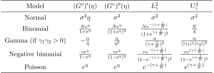
The first statement, (2), in Assumption 2 ensures that the distributions of Xijv have uniformly bounded variances and sub-exponential tails (see Lemma 28 in Appendix C). The second one, (3), is the strong convexity condition satisfied by the log-partition function Gv. This assumption is satisfied for most standard distributions presented in the previous section. In Table 1, we list the corresponding constants in Assumption 2.
Model (Gv)0(η) (Gv)00(η) L2γ Uγ2
Normal σ2η σ2 σ2 σ2
Binomial 1+eN eηη N e η
(1+eη)2 N e
−(γ+ 1K)
(1+eγ+ 1K)2
N 4 Gamma (ifγ1γ2 >0) −αη ηα2 (γ+α1
K)2
α (|γ1|∧|γ2|)2 Negative binomial 1−ereηη re
η
(1−eη)2 re
−(γ+ 1K)
(1−e−(γ+ 1K))2
re(γ+ 1K) (1−eγ+ 1K)2 Poisson eη eη e−(γ+K1) e(γ+
1 K)
Table 1: Examples of the corresponding constants L2γ andUγ2 from Assumption 2.
3.1. Estimation procedure
To estimate the collection of matrices of parametersM= (M1, . . . ,MV), we use penalized negative log-likelihood. Let W ∈ Rdu×D, we divide it in V blocks Wv ∈
Rdu×dv: W =
(W1, . . . ,WV). Given observationsY = (Y1, . . . ,YV), we write the negative log-likelihood as
LY(W) =− 1
duD
X
v∈[V]
X
(i,j)∈[du]×[dv]
Bvij YijvWijv −Gv(Wijv).
The nuclear norm penalized estimatorMc of Mis defined as follows:
c
M= (Mc1, . . . ,McV) = argmin
W∈C∞(γ)
LY(W) +λkWk∗, (4)
whereλis a positive regularization parameter that balances the trade-off between model fit and privileging a low-rank solution. Namely, for large value ofλthe rank of the estimator
c
Mis expected to be small.
where it equals to 1.For (εvij), ani.i.dRademacher sequence, we defineΣR= (Σ1R, . . . ,ΣVR) where for allv∈[V]
ΣvR= 1 duD
X
(i,j)∈[du]×[dv]
εvijBvijEvij.
We now state the main result concerning the recovery ofM. Theorem 3 gives a general upper bound on the estimation error of Mc defined by (4). Its proof is postponed in Appendix A.1.
Theorem 3 Assume that Assumptions 1 and 2 hold, and λ≥ 2k∇LY(M)k. Then, with
probability exceeding 1−4/(du+D) we have
1
duDkMc −Mk 2 Π,F ≤
c
pmax
n
duDrank(M)
λ2
L4 γ
+γ2(E[kΣRk])2
,γ
2log(du+D) duD
o
,
where
c
is a numerical constant.Using Assumption 1, Theorem 3 implies the following bound on the estimation error measured in normalized Frobenius norm.
Corollary 4 Under assumptions of Theorem 3 and with probability exceeding1−4/(du+D), we have
1 duDk
c
M−Mk2 F ≤
c
p2max
n
duDrank(M)
λ2
L4 γ
+γ2(E[kΣRk])2
,γ 2log(d
u+D) duD
o
.
In order to get a bound in a closed form we need to obtain a suitable upper bounds on E[kΣRk] and on k∇LY(M)k with high probability. Therefore we use the following two lemmas.
Lemma 5 There exists an absolute constant
c
such thatE[kΣRk]≤
c
√µ+plog(du∧D)
duD
.
Lemma 6 Let Assumption 2 holds. Then, there exists an absolute constant
c
such that,with probability at least 1−4/(du+D), we have
k∇LY(M)k ≤
c
(Uγ
∨K) √µ+ (log(du∨D))3/2 duD
.
The proofs of Lemmas 5 and 6 are postponed to Appendices A.2 and A.3. Recall that the condition onλin Theorem 3 is thatλ≥2k∇LY(M)k.Using Lemma 6, we can choose
λ= 2
c
(Uγ∨K)√µ+ (log(du∨D))3/2 duD .
Theorem 7 Let Assumptions 1 and 2 be satisfied. Then, with probability exceeding 1−
4/(du+D) we have
1
duDkMc −Mk 2 Π,F ≤
c
rank(M) pduD
γ2+ (Uγ∨K) 2 L4
γ
µ+ log3(du∨D)
,
and
1 duDk
c
M−Mk2F ≤
c
rank(M) p2duD
γ2+(Uγ∨K) 2 L4
γ
µ+ log3(du∨D)
,
where
c
is an absolute constant.Remark 8 Note that the rate of convergence in Theorem 7 has the following dominant term:
1
duDkMc −Mk 2 F .
rank(M)µ p2duD ,
where the symbol . means that the inequality holds up to a multiplicative constant. If we
assume that the sampling distribution is close to the uniform one, that is that there exists
positive constants c1 and c2 such that for every v ∈ [V] and (i, j) ∈ [du]×[dv] we have
c1p≤πvij ≤c2p, then Theorem 7 yields
1
duDkMc −Mk 2 F .
rank(M) p(du∧D).
If we complete each matrix separately, the error will be of the orderPVv=1rank(Mv)/p(du∧
D). As rank(M)≤PVv=1rank(Mv), the rate of convergence achieved by our estimator is faster compared to the penalization by the sum-nuclear-norm.
In order to get a small estimation error, p should be larger than rank(M)/(du∧D).
We denote n =Pv∈[V]P(i,j)∈[du]×[dv]πvij, the expected number of observations. Then, we
get the following condition on n:
n≥
c
rank(M)(du∨D).Remark 9 In1-bit matrix completion (Davenport et al., 2014; Klopp et al., 2015; Alquier
et al., 2017), instead of observing the actual entries of the unknown matrixM∈Rd×D, for
a random subset of its entries Ω we observe {Yij ∈ {+1,−1} : (i, j) ∈ Ω}, where Yij = 1
with probability f(Mij) for some link-function f. In Davenport et al. (2014) the parameter
Mis estimated by minimizing the negative log-likelihood under the constraintskMk∞≤γ
andkMk∗ ≤γ
√
rdDfor somer >0. Under the assumption thatrank(M)≤r,the authors
prove that
1
dDkMc −Mk 2 F ≤
c
γr
r(d∨D)
n , (5)
where
c
γis a constant depending onγ(see Theorem 1 in Davenport et al. (2014)). A similar2015) the authors prove a faster rate. Their upper bound (see Corollary 2 in Klopp et al. (2015)) is given by
1
dDkMc −Mk 2 F ≤
c
γrank(M)(d∨D) log(d∨D)
n . (6)
In the particular case of1-bit matrix completion for a single matrix under uniform sampling
scheme, Theorem 7 implies the following bound:
1
dDkMc −Mk 2 F ≤
c
γrank(M)(d∨D) n ,
which improves (6) by a logarithmic factor. Furthermore, Klopp et al. (2015) provide
rank(M)(d∨D)/n as the lower bound for1-bit matrix completion (see Theorem 3 in Klopp et al. (2015)). So our result answers the important theoretical question what is the exact
minimax rate of convergence for 1-bit matrix completion which was previously known up to
a logarithmic factor.
In a more general setting of matrix completion with exponential family noise, the mini-max optimal rate of convergence was also known only up to logarithmic factor (see Lafond (2015)). Our result provides the exact minimax optimal rate in this more general setting too. It is easy to see, by inspection of the proof of the lower bound in Lafond (2015), that the upper bound provided by Theorem 7 is optimal for the collective matrix completion.
Remark 10 Note that our estimation method is based on the minimization of the
nuclear-norm of the whole collective matrixM. Another possibility is to penalize by the sum of the
nuclear norms Pv∈[V]kMvk∗ (see, e.g., Klopp et al. (2015)). This approach consists in
estimating each component matrix independently.
4. General losses
In the previous section we assume that the link functionsGv are known. This assumption is not realistic in many applications. In this section we relax this assumption in the sense that we do not assume any specific model for the observations. Recall that our observations are a collection of partially observed matrices Yv = (BijvXi,jv ) ∈ Rdu×dv for v = 1, . . . , V
and Xv = (Xijv)∈Rdu×dv. We are interested in the problem of prediction of the entries of
the collective matrixX = (X1, . . . ,XV). We consider the risk of estimatingXv with a loss function `v, which measures the discrepancy between the predicted and actual value with respect to the given observations. We focus on non-negative convex loss functions that are Lipschitz:
Assumption 3 (Lipschitz loss function) For every v∈[V], we assume that the loss
func-tion `v(y,·) is ρv-Lipschitz in its second argument: |`v(y, x)−`v(y, x0)| ≤ρv|x−x0|.
For a matrix M= (M1, . . . ,MV)∈Rdu×D, we define the empirical risk as RY(M) =
1 duD
X
v∈[V]
X
(i,j)∈[du]×[dv]
Bijv`v(Yijv, Mijv).
We define the oracle as: ?
M= M?1, . . . ,M?V= argmin
Q∈C∞(γ)
R(Q) (7)
where R(Q) = E[RY(Q)]. Here the expectation is taken over the joint distribution of
{(Yijv, Bijv) : (i, j) ∈ [du]×[dv] and v ∈ [V]}. We use machine learning approach and will provide an estimator Mc that predicts almost as well as M?. Thus we will consider excess
risk R(Mc)−R(M?). By construction, the excess risk is always positive.
For a tuning parameter Λ>0, the nuclear norm penalized estimatorMc is defined as
c
M∈ argmin
Q∈C∞(γ)
RY(Q) + ΛkQk∗ . (8)
We next turn to the assumption needed to establish an upper bound on the performance of the estimator Mc defined in (8).
Assumption 4 Assume that there exists a constant
ς
>0such that for everyQ∈C∞(γ),we have
R(Q)−R(M?)≥
ς
duDkQ−M?k2Π,F.
This assumption has been extensively studied in the learning theory literature (Mendelson, 2008; Zhang, 2004; Bartlett et al., 2004; Alquier et al., 2017; Elsener and van de Geer, 2018), and it is called “Bernstein” condition. It is satisfied in various cases of loss function (Alquier et al., 2017) and it ensures a sufficient convexity of the risk around the oracle defined in (7). Note that when the loss function`v is strongly convex, the risk function inherits this property and automatically satisfies the margin condition. In other cases, this condition requires strong assumptions on the distribution of the observations, for instance for hinge loss or quantile loss (see Section 6 in Alquier et al. (2017)). The following result gives an upper bound on the excess risk of the estimatorMc.
Theorem 11 Let Assumptions 1, 3 and 4 hold and set ρ = maxv∈[V]ρv. Suppose that Λ≥2 sup{kGk:G ∈∂RY(
?
M)}.Then, with probability at least 1−4/(du+D), we have
R(Mc)−R(M?)≤
c
pmax
n
rank(M?)duD
ρ3/2pγ/
ς
(E[kΣRk])2+Λ 2ς
,
ργ+ρ3/2pγ/
ς
log(du+D) duDo
.
Theorem 11 gives a general upper bound on the prediction error of the estimator Mc. Its proof is presented in Appendix A.4. In order to get a bound in a closed form we need to
obtain a suitable upper bounds on sup{kGk:G ∈∂(RY(
?
Lemma 12 Let Assumption 3 holds. Then, there exists an absolute constant
c
such that,with probability at least 1−4/(du+D), we have
kGk ≤
c
ρ√µ+plog(du∨D)
duD
,
for all G∈∂RY(
? M).
The proof of Lemma 12 is given in Appendix A.5. Using Lemma 12 , we can choose
Λ = 2
c
ρ√µ+plog(du∨D)
duD
and with this choice of Λ and Lemma 5, we obtain the following theorem:
Theorem 13 Let Assumptions 1, 3 and 4 hold. Then, we have
R(Mc)−R(M?)≤
c
prank( ? M)(ρ
2+ρ3/2pγ/
ς
)(µ+ log(du∨D)) duD ,
with probability at least 1−4/(du+D).
Using Assumption 4, we get the following corollary:
Corollary 14 With probability at least1−4/(du+D), we have 1
duDkMc − ?
Mk2F ≤
c
p2
ς
rank( ? M)(ρ2+ρ3/2pγ/
ς
)(µ+ log(du∨D)) duD .
1-bit matrix completion. In 1-bit matrix completion with logistic (resp. hinge) loss, the Bernstein assumption is satisfied with
ς
= 1/(4e2γ) (resp.ς
= 2τ, for some τ that verifies |M?ijv −1/2| ≥ τ,∀v∈[V],(i, j)∈[du]×[dv]). More details for these constants can be found in Propositions 6.1 and 6.3 in Alquier et al. (2017). Then, the excess risk with respect to these two losses under the uniform sampling is given by:Corollary 15 With probability at least1−4/(du+D), we have
R(Mc)−R(M?)≤
c
rank(? M) p(du∧D).
These results are obtained without a logarithmic factor, and it improves the ones given in Theorems 4.2 and 4.4 in Alquier et al. (2017). The natural loss in this context is the 0/1 loss which is often replaced by the hinge or the logistic loss. We assume without loss of generality thatγ = 1, since the Bayes classifier has its entries in [−1,1], and we define the classification excess risk by:
R0/1(M) = 1 duD
X
v∈[V]
X
(i,j)∈[du]×[dv]
πijvP[Xijv 6= sign(Mijv)],
for all M∈Rdu×D.Using Theorem 2.1 in Zhang (2004), we have
R0/1(Mc)−R0/1(M?)≤
c
v u u
5. Numerical experiments
In this section, we first provide algorithmic details of the numerical procedure for solving the problem (4), then we conduct experiments on synthetic data to further illustrate the theoretical results of the collective matrix completion.
5.1. Algorithm
The collective matrix completion problem (4) is a semidefinite program (SDP), since it is a nuclear norm minimization problem with a convex feasible domain (Fazel et al., 2001; Srebro et al., 2005). We may solve it, for example, via the interior-point method (Liu and Vandenberghe, 2010). However, SDP solvers can handle a moderate dimensions, thus such formulation is not scalable due to the storage and computation complexity in low-rank matrix completion tasks. In the following, we present an algorithm that solves the problem (4) approximately and in a more efficient way than solving it as SDP.
Proximal Gradient. Problem (4) can be solved by first-order optimization methods such as proximal gradient (PG) which has been popularly used for optimizations problems of the form of (4) (Beck and Teboulle, 2009; Nesterov, 2013; Parikh and Boyd, 2014; Ji and Ye, 2009b; Mazumder et al., 2010; Yao and Kwok, 2015). WhenLY hasL-Lipschitz continuous gradient, that is k∇LY(W)− ∇LY(Q)kF ≤LkW−QkF, the PG generates a sequence of estimates {Wt}as
Wt+1= argmin
W LY
(W) + (W−Wt)>∇LY(Wt) + L
2kW−Wtk 2
F +λkWk∗
= proxλ Lk·k∗
(Zt), where Zt=Wt− 1
L∇LY(Wt) (9)
and for any convex function Ψ : Rdu×D 7→ R, the associated proximal operator at W ∈ Rdu×D is defined as
proxΨ(W) = argmin1
2kW−Qk 2
F + Ψ(Q) :Q∈Rdu×D .
The proximal operator of the nuclear norm atW ∈Rdu×D corresponds to the singular value thresholding (SVT) operator of W (Cai. et al., 2010). That is, assuming a singular value decomposition W = UΣV>, where U ∈ Rdu×r, V ∈ RD×r have orthonormal columns, Σ= (σ1, . . . , σr), withσ1≥ · · · ≥σr>0 andr= rank(W), we have
SVTλ/L(W) =Udiag((σ1−λ/L)+, . . . ,(σr−λ/L)+)V>, (10) where (a)+= max(a,0).
Although PG can be implemented easily, it converges slowly when the Lipschitz constant Lis large. In such scenarios, the rate isO(1/T), whereT is the number of iterations (Parikh and Boyd, 2014). Nevertheless, it can be accelerated by replacing Zt in (9) with
Qt= (1 +θt)Wt−θtWt−1, Zt=Qt−η∇LY(Qt). (11)
Algorithm 1:APG for Collective Matrix Completion 1. initialize: W0 =W1 =Y,andα0 =α1 = 1. 2. for t= 1, . . . , T do
3. Qt=Wt+αt−α1−1t (Wt−Wt−1);
4. Wt+1= SVTλ L(
Qt−L1∇LY(Qt)); 5. αt+1= 12(p4α2t + 1 + 1);
6. return WT+1.
Approximate SVT (Yao and Kwok, 2015). To computeWt+1 in the proximal step (SVT) in Algorithm 1, we need first perform SVD ofZtgiven in (11). In general, obtaining the SVD ofdu×DmatrixZtrequiresO((du∧D)duD) operations, because its most expensive steps are computing matrix-vector multiplications. Since the computation of the proximal operator of the nuclear norm given in (10) does not require to do the full SVD, only a few singular values of Zt which are larger than λ/L are needed. Assume that there are ˆ
k such singular values. As Wt converges to a low-rank solution W∗, ˆk will be small during iterating. The power method (Halko et al., 2011) at Algorithm 2 is a simple and efficient to capture subspace spanned by top-k singular vectors for ˆk ≥ k. Additionally, the power method also allows warm-start, which is particularly useful because the iterative nature of APG algorithm. Once an approximation Q is found, we have SVTλ/L(Zt) = QSVTλ/L(Q>Zt) (see Proposition 3.1 in Yao and Kwok (2015)). We therefore reduce the time complexity on SVT from O((du∧D)duD) to O(ˆkduD) which is much cheaper.
Algorithm 2:Power Method: PowerMethod(Z,R, )
1. input: Z ∈Rdu×D, initialR∈RD×k for warm-start, tolerance δ; 2. initialize W1 =ZR;
3. for t= 1,2, . . . ,do
4. Qt+1= QR(Wt);// QR denotes the QR factorization
5. Wt+1=Z(Z>Qt+1);
6. if kQt+1Q>t+1−QtQ>t kF ≤δ then break;
7. return Qt+1.
Algorithm 3 shows how to approximate SVTλ/L(Zt). Let the target (exact) rank-kSVD of Zt beUkΣkV>k. Step 1 first approximates Uk by the power method. In steps 2 to 5, a less expensive SVTλ/L(Q>Zt) is obtained from (10). Finally, SVTλ/L(Zt) is recovered.
Hereafter, we denote the objective function in (4) by Fλ(W), that is Fλ(W) =
LY(W) +λkWk∗, for any W ∈ C(γ). Recall that the gradient of the likelihood LY is written as
∇LY(W) =− 1
duD
X
v∈[V]
X
(i,j)∈[du]×[dv]
Algorithm 3:Approximate SVT: Approx-SVT(Z,R, λ, δ) 1. input: Z ∈Rdu×D,R∈
RD×k,thresholds λandδ;
2. Q=PowerMethod(Z,R, δ);
3. [U,Σ,V] = SVD(Q>Z); 4. U ={ui|σi > λ};
5. V ={vi|σi> λ};
6. Σ= max(Σ−λI,0); // (I denotes the identity matrix) 7. return QU,Σ,V.
By Assumption 2, we have for anyW,Q∈Rdu×D
k∇LY(W)− ∇LY(Q)k2
F = 1 (duD)2
X
v∈[V]
X
(i,j)∈[du]×[dv]
{Bijv((Gv)0(Wijv)−(Gv)0(Qvij))}2
≤ U
2 γ
(duD)2kW−Qk 2 F.
This yields that LY has L-Lipschitz continuous gradient with L=Uγ/(duD) ≤1. In the following algorithm and the experimental setup, we choose to work withL= 1.
Penalized Likelihood Accelerated Inexact Soft Impute (PLAIS-Impute). We present here the main algorithm in this paper, referred to as PLAIS-Impute, which is tailored to solving our collective matrix completion problem. The PLAIS-Impute is an adaption of the AIS-Impute algorithm in Yao and Kwok (2015) to the penalized likelihood completion problems. Note that AIS-Impute is an accelerated proximal gradient algorithm with further speed up based on approximate SVD. However, it is dedicated only to square-loss goodness-of-fitting. The PLAIS-Impute is summarized in Algorithm 4. The core steps are 10-12, where an approximate SVT is performed. Steps 10 and 11 use the column space of the last iterations (Vt and Vt−1) to warm-start the power method. For further speed up, a continuation strategy is employed in whichλt is initialized to a large value and then decreases gradually. The algorithm is restarted (at the step 14) if the objective function
Fλ starts to increase. As AIS-Impute, PLAIS-Impute shares both low-iteration complexity and fastO(1/T2) convergence rate (see Theorem 3.4 in Yao and Kwok (2015)).
5.2. Synthetic datasets
Software. The implementation of Algorithm 4 for the nuclear norm penalized estima-tor (4) was done in MATLAB R2017b on a desktop computer with macOS system, Intel i7 Core 3.5 GHz CPU and 16GB of RAM. For fast computation of SVD and sparse matrix computations, the experiments call an external package called PROPACK (Larsen, 1998) implemented in C and Fortran. The code that generates all figures given below is available
from https://github.com/mzalaya/collectivemc.
Algorithm 4:PLAIS-Impute for Collective Matrix Completion
1. input: observed collective matrixY, parameter λ, decay parameter ν∈(0,1), toleranceε;
2. [U0, λ0,V0] = rank-1 SVD(Y);
3. initialize c= 1, δ0 =kYkF,W0 =W1=λ0U0V>0; 4. for t= 1, . . . , T do
5. δt=νtδ0;
6. λt=νt(λ0−λ) +λ; 7. θt= (c−1)/(c+ 2);
8. Qt= (1 +θt)Wt−θtWt−1;
9. Zt=∇LY(Qt));
10. Vt−1 =Vt−1−Vt(V>t Vt−1); 11. Rt= QR([Vt,Vt−1]);
12. [Ut+1,Σt+1,Vt+1] =Approx-SVT(Zt,Rt, λt, δt); 13. if Fλ(Ut+1Σt+1V>t+1)>Fλ(UtΣtV>t ) then
c= 1;
14. else
c=c+ 1;
15. if |Fλ(Ut+1Σt+1V>t+1)−Fλ(UtΣtV>t )| ≤εthen break;
16. return WT+1.
dv ∈ {1000,2000,3000} (hence d=D=P3v=1dv). Each source matrix Mv is constructed as Mv = LvRv> where Lv ∈
Rd×rv and Rv ∈ Rdv×rv. This gives a random matrix of
rank at most rv. The parameter rv is set to{5,10,15}. A fraction of the entries of Mv is removed uniformly at random with probabilityp∈[0,1]. Then, the matricesMv are scaled so that kMvk
∞=γ = 1.
For M1, the elements of L1 and R1 are sampled i.i.d. from the normal distribution
N(0.5,1). ForM2, the entries ofL2andR2are i.i.d. according to Poisson distribution with parameter 0.5. Finally, for M3, the entries of L3 and R3 are i.i.d. sampled from Bernoulli distribution with parameter 0.5. The collective matrixMis constructed by concatenation of the three sources M1,M2 and M3, namely M = (M1,M2,M3). All the details of these experiments are given in Table 2.
M1 M2 M3 M (Gaussian) (P oisson) (Bernoulli) (Collective)
exp.1
dimension 3000×1000 3000×1000 3000×1000 3000×3000
rank 5 5 5 unknown
exp.2
dimension 6000×2000 6000×2000 6000×2000 6000×6000
rank 10 10 10 unknown
exp.3
dimension 9000×3000 9000×3000 9000×3000 9000×9000
rank 15 15 15 unknown
Table 2: Details of the synthetic data in the three experiments.
0 10 20 30
Times (seconds) 0 100 101 102 103 104 105 Fλ
d= 3000
Collective Gaussian Poisson Bernoulli
0 50 100 150 200
Times (seconds) 0 100 101 102 103 104 105 106
d= 6000
Collective Gaussian Poisson Bernoulli
0 100 200 300 400 500 600 Times (seconds) 0 100 101 102 103 104 105 106
d= 9000
Collective Gaussian Poisson Bernoulli
−5 0 5 10 15 20
−log(λ)
0 100 101 102 103 104 105 Fλ
d= 3000
Collective Gaussian Poisson Bernoulli
−5 0 5 10 15 20
−log(λ)
0 100 101 102 103 104 105 106
d= 6000
Collective Gaussian Poisson Bernoulli
−5 0 5 10 15 20
−log(λ)
0 100 101 102 103 104 105 106
d= 9000
Collective Gaussian Poisson Bernoulli
0 5 10 15 Iterations
5 10 15 20 25
Lea
rned
ranks
d= 3000
RanksIn RanksOut
0 5 10 15
Iterations 10
20 30 40 50
Lea
rned
ranks
d= 6000
RanksIn RanksOut
0 5 10 15 20
Iterations 10
20 30 40 50 60 70
Lea
rned
ranks
d= 9000
RanksIn RanksOut
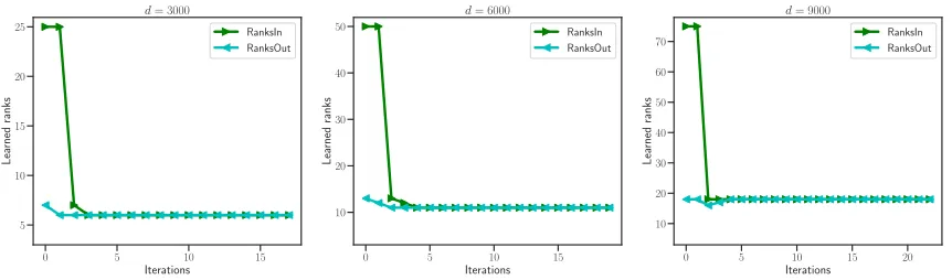
Figure 2: Learning ranks curve versus iterations in the three experiments with p = 0.6; left for exp.1; middle forexp.2; right for exp.3. We initialize the algorithm by setting a rank r0 = 5r where r ∈ {5,10,15}.The green color corresponds to the input rank while the cyan to the recovered rank of the collective matrix at each iteration. As can be seen, the two ranks gradually converge to the final recovered rank.
Evaluation. In our experiments, the PLAIS-Impute algorithm terminates when the ab-solute difference in the cost function values between two consecutive iterations is less than = 10−6. We set the regularization parameter λ∝ k∇LY(M)k as given by Theorem 3. Note that in step 12 of PLAIS-Impute, the threshold in SVT is given by λt (defined in step 6), which is decreasing from one iteration to another. This allows to tune the first regularization parameter λin the program (4). We randomly sample 80% of the observed entries for training, and the rest for testing.
In order to measure the the accuracy of our estimator, we employ the relative error (as, e.g., in Cai. et al. (2010); Davenport et al. (2014); Cai and Zhou (2013)) which is widely used metric in matrix completion and is defined by
RE(Wc,W) = kWc −W ok
F
kWok
F ,
whereWc is the recovered matrix andWo is the original full data matrix.
We run the PLAIS-Impute algorithm in each experiment by varying the percentage of known entries p from 0 to 1. In Figure 3, we plot the relative errors as a functions of p. We observe in Figure 3 that the relative errors are decaying with p. Note that for each v ∈ {1,2,3}, the estimator Mdv is calculated separately using the same program (4). The results shown in Figure 3 confirm that collective matrix completion approach outperforms the approach that consists in estimating each component source independently.
Cold-Start problem. To simulate cold-start scenarios, we choose one of the source ma-tricesMv to be “cold” by increasing its sparsity. More precisely, we proceed in the following way: we extract vector of known entries of the chosen matrix and we set the first 1/5 fraction of its entries to be equal to 0.We denote the obtained matrix by Mcoldv and the collective matrix by Mv
cold. In exp.1, exp.2 and exp.3, we increase the sparsity of M1, M2, and
M3, respectively. Hence, we get the “cold” collective matricesM1cold= (Mcold1 ,M2,M3), M2
0.2 0.4 0.6 0.8 1.0 Percentage of known entries 0.5
0.6 0.7 0.8 0.9 1.0
Relative
erro
rs
d= 3000
Collective Gaussian Poisson Bernoulli
0.2 0.4 0.6 0.8 1.0 Percentage of known entries 0.6
0.7 0.8 0.9 1.0
Relative
erro
rs
d= 6000
Collective Gaussian Poisson Bernoulli
0.2 0.4 0.6 0.8 1.0 Percentage of known entries 0.60
0.65 0.70 0.75 0.80 0.85 0.90 0.95 1.00
Relative
erro
rs
d= 9000
Collective Gaussian Poisson Bernoulli
Figure 3: Performance on the synthetic data in terms of relative errors between the target and the estimator matrices as a function of the percentage of known entries p from 0 to 1.
We run 10 times the PLAIS-Impute algorithm for recovering the source Mcoldv and the collective Mvcold for eachv= 1,2,3. We denote byM\v
compthe estimator of Mcoldv obtained by running the PLAIS-Impute algorithm only for this component. Analogously, we denote
\
Mcollectv the estimator of Mcoldv obtained by extracting the v-th source of the collective estimator M\v
cold.
In Figure 4, we report the relative errors RE(M\v
comp,Mcoldv ) and RE(M\collectv ,Mcoldv ) in the three experiments. We see that, the collective matrix completion approach compensates the lack of informations in the “cold” source matrix. Therefore, this shared structure among the sources is useful to get better predictions.
d= 3000 d= 6000 d= 9000 Dimensions
0.0 0.2 0.4 0.6 0.8 1.0
Relative
erro
rs RE(Mccollect1 , Mcold1 )
RE(Mc1
comp, Mcold1 )
RE(Mc2
collect, Mcold2 )
RE(Mc2
comp, Mcold2 )
RE(Mc3
collect, Mcold3 )
RE(Mc3
comp, Mcold3 )
6. Conclusion
This paper studies the problem of recovering a low-rank matrix when the data are collected from multiple and heterogeneous source matrices. We first consider the setting where, for each source, the matrix entries are sampled from an exponential family distribution. We then relax this assumption. The proposed estimators are based on minimizing the sum of a goodness-of-fit term and the nuclear norm penalization of the whole collective matrix. Allowing for non-uniform sampling, we establish upper bounds on the prediction risk of our estimator. As a by-product of our results, we provide exact minimax optimal rate of convergence for 1-bit matrix completion which previously was known upto a logarithmic factor. We present the proximal algorithm PLAIS-Impute to solve the corresponding convex programs. The empirical study provides evidence of the efficiency of the collective matrix completion approach in the case of joint low-rank structure compared to estimate each source matrices separately.
Acknowledgment
Appendix A. Proofs
We provide proofs of the main results, Theorems 3 and 11, in this section. The proofs of a few technical lemmas including Lemmas 5, 6 and 12 are also given. Before that, we recall some basic facts about matrices.
Basic facts about matrices. The singular value decomposition (SVD) of A has the form A = Prank(A)l=1 σl(A)ul(A)vl>(A) with orthonormal vectors u1(A), . . . , urank(A)(A), orthonormal vectorsv1(A), . . . , vrank(A)(A), and real numbersσ1(A)≥ · · · ≥σrank(A)(A)> 0 (the singular values ofA). Let (S1(A),S2(A)) be the pair of linear vectors spaces, where
S1(A) is the linear span space of {u1(A), . . . , urank(A)(A)}, and S2(A) is the linear span space of {v1(A), . . . , vrank(A)(A)}. We denote by Sj⊥(A) the orthogonal complements of
Sj(A), forj = 1,2 and by PS the projector on the linear subspaceS of Rn orRm.
For two matrices A and B, we set PA⊥(B) = PS⊥
1(A)BPS2⊥(A) and PA(B) = B −
P⊥
A(B). Since PA(B) =PS1(A)B+PS⊥
1 (A)BPS2(A), and rank(PSj(A)B) ≤rank(A), we have that
rank(PA(B))≤2 rank(A). (12)
It is easy to see that for two matrices Aand B (Klopp, 2014)
kAk∗− kBk∗ ≤ kPA(A−B)k∗− kPA⊥(A−B)k∗. (13)
Finally, we recall the well-known trace duality property: for allA,B∈Rn×m, we have
|hA,Bi| ≤ kBkkAk∗.
A.1. Proof of Theorem 3
First, noting thatMc is optimal andMis feasible for the convex optimization problem (4), we thus have the basic inequality that
1 duD
X
v∈[V]
X
(i,j)∈[du]×[dv]
Bijv Gv( ˆMijv)−YijvMˆijv+λkMck∗
≤ 1
duD
X
v∈[V]
X
(i,j)∈[du]×[dv]
Bijv Gv(Mijv)−YijvMijv+λkMk∗.
It yields
1 duD
X
v∈[V]
X
(i,j)∈[du]×[dv]
Bijv Gv( ˆMijv)−Gv(Mijv)−Yijv Mˆijv −Mijv≤λ(kMk∗− kMck∗).
Using the Bregman divergence associated to each Gv, we get
1 duD
X
v∈[V]
X
(i,j)∈[du]×[dv]
BijvdGv( ˆMijv, Mijv)
≤λ(kMk∗− kMck∗)−
1 duD
X
v∈[V]
X
(i,j)∈[du]×[dv]
Therefore, using the duality betweenk · k∗ and k · k, we arrive at
1 duD
X
v∈[V]
X
(i,j)∈[du]×[dv]
BijvdGv( ˆMijv, Mijv)≤λ(kMk∗− kMck∗)− h∇LY(M),Mc −Mi
≤λ(kMk∗− kMck∗) +k∇LY(M)kkMc −Mk∗.
Besides, using the assumptionλ≥2k∇LY(M)kand inequality (13) lead to
1 duD
X
v∈[V]
X
(i,j)∈[du]×[dv]
BijvdGv( ˆMijv, Mijv)≤ 3λ
2 kPM Mc −M
k∗.
Since kPA(B)k∗ ≤
p
2 rank(A)kBkF for any two matricesA and B, we obtain
1 duD
X
v∈[V]
X
(i,j)∈[du]×[dv]
BijvdGv( ˆMijv, Mijv)≤ 3λ 2
p
2 rank(M)kMc −MkF. (14)
Now, Assumption 2 implies that the Bregman divergence satisfiesL2γ(x−y)2≤2dvG(x, y)≤ U2
γ(x−y)2,then we get
∆2Y(M,c M)≤
2 L2
γ 1 duD
X
v∈[V]
X
(i,j)∈[du]×[dv]
BijvdGv( ˆMijv, Mijv), (15)
where
∆2Y(M,c M) =
1 duD
X
v∈[V]
X
(i,j)∈[du]×[dv]
Bijv( ˆMijv −Mijv)2.
Combining (14) and (15), we arrive at
∆2Y(M,c M)≤
3λ L2 γ
p
2 rank(M)kMc −MkF. (16)
Let us now define the threshold β = 946γ2log(du+D)
pduD and distinguish the two following cases that allows us to obtain an upper bound for the estimation error:
Case 1: if (duD)−1kMc −Mk2
Π,F < β, then the statement of Theorem 3 is true.
Case 2: it remains to consider the case (duD)−1kMc −Mk2
Π,F ≥ β. Lemma 18 in Ap-pendix B.1 implies kMc −MkF ≥ 1
4√2 rank(M)kMc −Mk∗, then we obtain
kMc −Mk∗ ≤
p
32 rank(M)kMc −MkF.
This leads toMc ∈C β,32 rank(M),where the set
C(β, r) =
W ∈C∞(γ) :kM−Wk∗ ≤√rkW−MkF and (duD)−1kW−Mk2Π,F ≥β
.
Using Lemma 19 in Appendix B.1, we have
∆2Y(M,c M)≥
kW −Mk2
Π,F
2duD −44536 rank(M)γ 2(
E[kΣRk])2−5567γ
2
duDp . (18)
Together (18) and (16) imply
1 2duDk
c
M−Mk2Π,F ≤ 3λ L2 γ
p
2 rank(M)kMc −MkF
+ 44536 rank(M)γ2(E[kΣRk])2+
5567γ2 pduD
≤ 18λ
2d uD pL4
γ
rank(M) + 1
4duDkMc −Mk 2 Π,F + 44536 rank(M)γ2(E[kΣRk])2+5567γ 2 pduD .
Then,
1 4duDk
c
M−Mk2 Π,F ≤
18λ2duD pL4
γ
rank(M)
+ 44536p−1duDrank(M)γ2(E[kΣRk])2+ 5567γ 2 duDp ,
and,
1 duDk
c
M−Mk2Π,F ≤p−1max
duDrank(M)
c1λ2 L4
γ
+c2γ2(E[kΣRk])2
,c3γ 2 duD
,
wherec1, c2 and c3 are numerical constants. This concludes the proof of Theorem 3. A.2. Proof of Lemma 5
We use the following result:
Proposition 16 (Corollary 3.3 in Bandeira and van Handel (2016)) LetW be the n×m
rectangular matrix whose entries Wij are independent centered bounded random variables.
Then there exists a universal constant
c
such thatE[kWk]≤
c
κ1∨κ2+κ∗p
log(n∧m),
where we have defined
κ1 = max i∈[n]
s X
j∈[m] E[W2
i,j], κ2= max j∈[m]
s X
i∈[n] E[W2
i,j], and κ∗ =(i,j)∈[n]×[m]max |Wij|. We apply Proposition 16 toΣR= du1DPv∈[V]
P
(i,j)∈[du]×[dv]ε v
ijBijvEijv. We compute
κ1= 1 duD
max i∈[du]
s X
v∈[V]
X
j∈[dv]
E[(εvij)2(Bv ij)2] =
1 duD
max i∈[du]
s X
v∈[V]
X
j∈[dv] πvij
= 1 duDi∈[dmaxu]
pπi
κ2= 1
duDv∈[Vmax]j∈[dmaxv]
s X
i∈[du]
E[(εvij)2(Bv ij)2] =
1
duDv∈[Vmax]j∈[dmaxv]
s X
i∈[du] πvij
≤ 1
duDj∈[dmaxv]
s
max v∈[V]
X
i∈[du] πv
ij
≤ d1
uD max j∈[dv]
pπ
·
j, and κ∗ = d1uDmaxv∈[V]max(i,j)∈[du]×[dv]|ε v
ijBij| ≤ du1D. Using inequality (1), we have κ1 ≤ √
µ
duD and κ2 ≤ √
µ
duD. Then,κ1∨κ2 ≤ √
µ
duD, which establishes Lemma 5.
A.3. Proof of Lemma 6 We write∇LY(M) =−d1 uD
P
v∈[V]
P
(i,j)∈[du]×[dv]H v
ijEijv, withHijv =Bijv Xijv−(Gv)0(Mijv)
. For a truncation levelT >0 to be chosen, we decompose∇LY(M) =Σ1+Σ2, where
Σ1 =− 1 duD
X
v∈[V]
X
(i,j)∈[du]×[dv]
Hijv1((Xv
ij−E[Xijv])≤T)−E
Hijv1((Xv
ij−E[Xijv])≤T)
Eijv,
and
Σ2 =− 1
duD
X
v∈[V]
X
(i,j)∈[du]×[dv]
Hijv1((Xv
ij−E[Xijv])>T)−E
Hijv1((Xv
ij−E[Xijv])>T)
Eijv,
then, the triangular inequality implies k∇LY(M)k ≤ kΣ1k+kΣ2k. Then, the proof is divided on two steps:
Step 1: control of kΣ1k. In order to control kΣ1k, we use the following bound on the
spectral norms of random matrices. It is obtained by extension to rectangular matrices via self-adjoint dilation of Corollary 3.12 and Remark 3.13 in Bandeira and van Handel (2016).
Proposition 17 (Bandeira and van Handel, 2016) LetW be then×mrectangular matrix
whose entries Wij are independent centered bounded random variables. Then, for any 0≤
≤1/2 there exists a universal constant
c
such that for every x≥0,PkWk ≥2√2(1 +)(κ1∨κ2) +x≤(n∧m) exp
− x
2
c
κ2 ∗
,
where κ1, κ2, and κ∗ are defined as in Proposition 16.
We apply Proposition 17 toΣ1. We compute
κ1= 1 duD
max i∈[du]
s X
v∈[V]
X
j∈[dv]
Eh Hv
ij1((Xvij−E[Xvij])≤T)−E
Hv
ij1((Xijv−E[Xijv])≤T)
2i
.
Besides, we have
Eh Hijv1((Xv
ij−E[Xijv])≤T)−E
Hijv1((Xv
ij−E[Xijv])≤T)
2i
≤E(Hijv)21((Xv
ij−E[Xijv])≤T)
and
E(Hijv)21((Xv
ij−E[Xijv])≤T)
=E(Bvij)2 Xijv −E[Xijv])21((Xv
ij−E[Xijv])≤T)
≤πijvVar[Xijv] =πijv(Gv)00(Mijv).
By Assumption 2, we obtain E(Hijv)21((Xv
ij−E[Xijv])≤T)
≤ πijvUγ2 for all v ∈ [V],(i, j) ∈ [du]×[dv]. Then,
κ1≤ Uγ duD
max i∈[du]
s X
v∈[V]
X
j∈[dv]
πijv ≤ Uγ duD
max i∈[du]
q
πvi
·
≤ Uγ√µ
duD ,
and
κ2≤ Uγ duD
max j∈[dv]
s
max v∈[V]
X
i∈[du]
πvij ≤ Uγ duD
max j∈[dv]
pπ
·
j ≤Uγ√µ duD
.
It yields, κ1∨κ2 ≤ Uγ
√ µ
duD . Moreover, we have E
Hijv1((Xv ij−E[X
v ij])≤T)
≤ T, which entails κ∗ ≤ d2T
uD. By choosing = 1/2 in Proposition 17, we obtain, with probability at least 1−4(du∧D)e−x2,
kΣ1k ≤ 3Uγ
√
2µ+ 2√
c
1/2xT duD .Therefore, by setting x=p2 log(du+D), we get with probability at least 1−4/(du+D),
kΣ1k ≤
3Uγ√2µ+ 2√
c
1/2p
2 log(du+D)T duD
. (19)
Step 2: control of kΣ2k. To controlkΣ2k, we use Chebyshev’s inequality, that is
PkΣ2k ≥E[kΣ2k] +x≤ Var[kΣ2k]
x2 , for all x >0. We start by estimatingE[kΣ2k]. We use the fact that E[kΣ2k]≤E[kΣ2kF]:
EkΣ2k2F= 1 (duD)2
X
v∈[V]
X
(i,j)∈[du]×[dv]
E Hijv1((Xv
ij−E[Xijv])>T)−E
Hijv1((Xv
ij−E[Xijv])>T)
2
≤ (d 1
uD)2
X
v∈[V]
X
(i,j)∈[du]×[dv]
E(Hijv)21((Xv
ij−E[Xijv])>T)
≤ 1
(duD)2
X
v∈[V]
X
(i,j)∈[du]×[dv]
πijvE(Xijv −E[Xijv])21((Xv
ij−E[Xijv])>T)
≤ 1
(duD)2
X
v∈[V]
X
(i,j)∈[du]×[dv] πijv
q
E(Xijv −E[Xijv])4qP((Xv
ij −E[Xijv])> T)
By Lemma 28, we have that Xijv −E[Xijv] is an (Uγ, K)-sub-exponential random variable for everyv∈[V] and (i, j)∈[du]×[dv]. It yields, using (2) in Theorem 26, that
E(Xijv −E[Xijv])p≤
c
ppkXijvkpψ1, for everyp≥1,and by (1) in Theorem 26
P|Xijv −E[Xijv]|> T≤exp
1− T
c
sekXijvkψ1
,
where
c
andc
se are absolute constants. Consequently, EkΣ2k2F
≤ (d
c
uD)2
X
v∈[V]
X
(i,j)∈[du]×[dv] πijv
q
kXijvk4ψ1
s
exp1− T
c
sekXijvkψ1
≤
c
(duD)2
X
v∈[V]
X
(i,j)∈[du]×[dv]
(Uγ∨K)2πvij
r
exp− T
c
seK
.
We chooseT =T∗ := 4
c
se(Uγ∨K) log(du∨D). It yields, EkΣ2k2F
≤ (d
c
uD)2 1 (du∨D)2
X
v∈[V]
X
(i,j)∈[du]×[dv]
(Uγ∨K)2πijv
≤
c
(Uγ∨K)2 (duD)2
1 (du∨D)2
X
v∈[V]
X
j∈[dv] πijv
≤
c
(Uγ∨K)2 (duD)2
1
(du∨D)2(du∨D)µ
≤
c
(Uγ∨K)2µ (duD)2du∨D. Using the fact that x7→√x is concave, we obtain
E[kΣ2k]≤E[kΣ2kF]≤
q
EkΣ2k2F
≤
s
c
(Uγ∨K)2µ (duD)2du∨D ≤c
(Uγ∨K)√µ duD√
du∨D
. (20)
Let us now control the variance of kΣ2k. We have immediately, using (20),
Var[kΣ2k]≤E[kΣ2k2]≤EkΣ2k2F≤
c
(Uγ∨K) 2µ (duD)2du∨D.
By Chebyshev’s inequality and using (20), we have, with probability at least 1−4/(du+D),
kΣ2k ≤
c
(Uγ∨K)√µ
duD√du∨D +
c
(Uγ∨K)√µ duD ≤c
(Uγ∨K)√µduD . (21)
Finally, combining (19) and (21), we obtain, with probability at least 1−4/(du+D),
k∇LY(M)k ≤
3Uγ√2µ+ 8(Uγ∨K)
c
seq
Then,
k∇LY(M)k ≤
c
(U
γ∨K) √µ+ (log(du∨D))3/2
duD
,
where
c
is an absolute constant. This finishes the proof of Lemma 6.A.4. Proof of Theorem 11
We start the proof with the following inequality using the fact thatMc is the minimizer of the objective function in problem (8)
0≤ −(RY(Mc) + ΛkMck∗) + (RY(
?
M) + ΛkM?k∗).
Then, by adding R(Mc)−R(M?)≥0, we obtain
R(Mc)−R(M?)≤ − RY(Mc)−RY(
?
M)− R(Mc)−R(M?) + Λ kM?k∗− kMck∗
.
(13) implieskAk∗− kBk∗ ≤ kPA(A−B)k∗ and we get
R(Mc)−R(M?)≤ − RY(Mc)−RY(
?
M)− R(Mc)−R(M?) + ΛkP ?
M(
?
M−Mc)k∗
≤ − RY(Mc)−RY(
?
M)+ R(Mc)−R(M?) (22)
+ Λ
q
2 rank(M?)kMc −M?kF.
Let us now define the threshold ν = 32 1+e
√
3ρ/
ς
γργlog(du+D)3pduD and distinguish the two following cases that allows us to obtain an upper bound for the prediction error:
Case 1: ifR(Mc)−R(M?)< ν, then the statement of Theorem 11 is true.
Case 2: it remains to consider the caseR(Mc)−R(M?)≥ν. Lemma 21 implies
kMc −M?k∗ ≤
q
32 rank(M?)kMc −M?kF,
thenMc ∈Q(ν,32 rank(M?)) where
Q(ν, r) =
Q∈C∞(γ) :kQ− ?
Mk∗≤√rkQ− ?
MkF and R(Q)−R(M?)≥ν
.
Using Lemma 22, we have
R(Mc)−R(M?)− RY(Mc)−RY(
? M)
≤ R(Mc)−R(
? M)
2 +
c
rank(M?)ρ2ς
−1(E[kΣ Rk])2Now, plugging (23) in (22), we get
R(Mc)−R(M?)≤
c
rank( ?M)ρ2
ς
−1(E[kΣ Rk])2(1/4e) + (1−1/√4e)p3ρ/4
ς
γ + 2Λq
2 rank(M?)kMc −M?kF,
where
c
= 1024. Then using the fact that for any a, b ∈ R, and > 0, we have 2ab ≤ a2/(2) + 2b2, we get for =pς
/4R(Mc)−R(M?)≤
c
duDp−1rank(M?)ρ2
ς
−1(E[kΣ Rk])2 (1/4e) + (1−1/√4e)p3ρ/4ς
γ+ Λ2duD(p
ς
/4)−1rank(M?) + pς
2duDkMc − ? Mk2F
≤
c
duDp−1rank(M?)ρ2
ς
−1(E[kΣRk])2 (1/4e) + (1−1/√4e)p3ρ/4
ς
γ+ Λ2duD(p
ς
/4)−1rank(M?) +ς
2duDkc
M−M?k2Π,F. Using Assumption 4, we obtain
R(Mc)−R(M?)≤ 2
c
duDp−1rank(M?)ρ2
ς
−1(E[kΣRk])2 (1/4e) + (1−1/√4e)p3ρ/4
ς
γ + 8Λ2d
uD(p
ς
)−1rank( ? M)≤(p
ς
)−1rank(M?)duDρ2(E[kΣ
Rk])2
(1/4e) + (1−1/√4e)p3ρ/4
ς
γ + 8Λ 2.This finishes the proof of Theorem 11.
A.5. Proof of Lemma 12
By the nonnegative factor and the sum properties of subdifferential calculus (Boyd and Vandenberghe, 2004), we write
∂RY(
? M) =
G = 1 duD
X
v∈[V]
X
(i,j)∈[du]×[dv]
BijvGvijEijv :Gvij ∈∂`v(Yijv,M?ijv)
Recall that the sudifferential of∂`v(Yijv,M?ijv) at the pointM?ijv is defined as
∂`v(Yijv,M?ijv) ={Gvij :`v(Yijv, Qvij)≥`v(Yijv,M?ijv) +Gvij(Qvij −M?ijv)}.
Thanks to Assumption 3, we have, for all Gvij ∈∂`v(Yijv,M?ijv)
|Gvij(Qvij −M?ijv)| ≤ |`v(Yijv, Qvij)−`v(Yijv,M?ijv)| ≤ρv|Qvij−M?ijv|,