Image Completion: Comparison of Different Methods and Combination of Techniques

University of New Orleans University of New Orleans

ScholarWorks@UNO

ScholarWorks@UNO

University of New Orleans Theses and

Dissertations Dissertations and Theses

5-20-2011

Image Completion: Comparison of Different Methods and

Image Completion: Comparison of Different Methods and

Combination of Techniques

Combination of Techniques

Lawrence LeBlanc

University of New Orleans

Follow this and additional works at: https://scholarworks.uno.edu/td

Recommended Citation Recommended Citation

LeBlanc, Lawrence, "Image Completion: Comparison of Different Methods and Combination of Techniques" (2011). University of New Orleans Theses and Dissertations. 1326.

https://scholarworks.uno.edu/td/1326

Image Completion: Comparison of Different Methods and Combination of Techniques

A Thesis

Submitted to the Graduate Faculty of the University of New Orleans in partial fulfillment of the requirements for the degree of

Master of Science

in

Engineering

by

Lawrence Leblanc

Table of Contents

List of Figures ... iii

List of Tables ... iv

Abstract ... v

Introduction ... 1

Related Work ... 2

Implemented Algorithms ... 3

Overview of Criminisi’s Exemplar Image completion Algorithm ... 3

Overview of Anupam's Algorithm ... 7

Overview of Kwok’s Exemplar Image Completion with Fast Query Algorithm ... 9

Overview of Proposed Algorithm ... 13

Results and Discussion ... 14

Conclusion ... 24

Bibliography ... 26

List of Figures

Figure 1: Criminisi's exemplar image completion algorithm ... 3

Figure 2: Anupam's image completion algorithm ... 9

Figure 3: Kwok's image completion algorithm ... 10

Figure 4: An example of least squares setup for gradient filling algorithm...11

Figure 5: Kwok's Fast Query Algorithm ... 13

Figure 6: Input images used in the comparisons. Missing Regions are shown in black patches. From left to right the images are: chimney, Lena Wall, Lena Hat, simple, and bricks. ... 15

Figure 7: Visual Quality comparison of Anupam's outputs with different values of Dx and Dy using Lena all image.. From left to right: Dx = Dy = 1, Dx = Dy = 9, and Dx = Dy = 27... 15

Figure 8: Visual Quality Comparison using Lens Wall image of Kwok's algorithm with different numbers of truncated coefficients. From left to right: m = 4, m = 8, and m = 40 ... 17

Figure 9: Visual comparison of simple image across all four algorithms. From left to right: Criminisi, Anupam, Kwok, and the proposed algorithm. ... 18

Figure 10: Visual comparison of chimney image across all four algorithms:Criminisi (a), Anupam (b), Kwok (c), and the proposed algorithm (d). ... 20

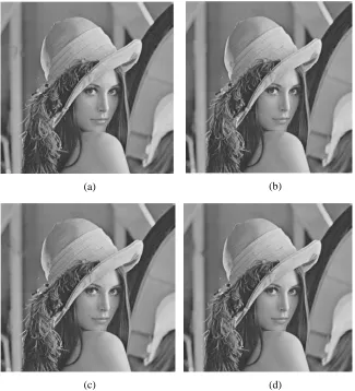
Figure 11: Visual comparison of Lena wall image across all four algorithms. Criminisi (a), Anupam (b), Kwok (c), and the proposed algorithm (d). ... 21

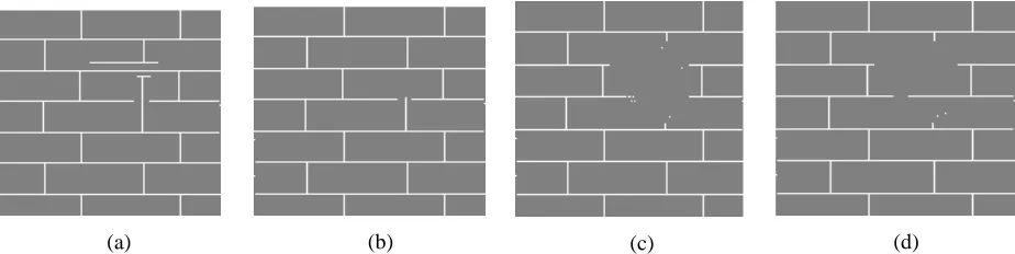
Figure 12: Visual comparison of bricks image across all four algorithms. Criminisi (a), Anupam (b), Kwok (c), and the proposed algorithm (d). ... 22

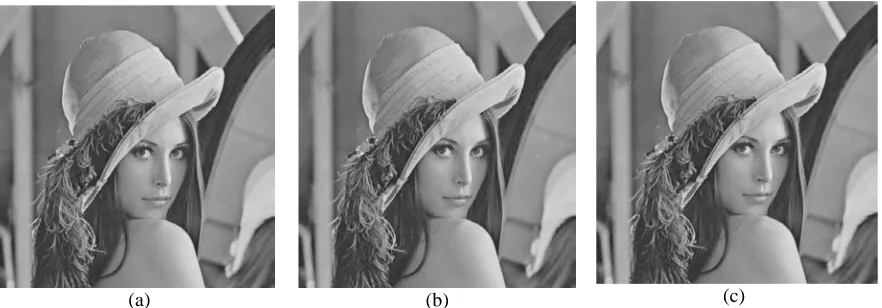
Figure 13: Visual comparison of Lena hat image across all four algorithms: Criminisi (a), Anupam (b), Kwok (c), and the proposed algorithm (d). ... 23

Figure 14: An Example of overshooting. Input image on the left and the output image from the proposed algorithm on the right. ... 24

List of Tables

Table 1: Timed execution comparison in seconds of Anupam's algorithm with different values for Dx and Dy. ... 15

Abstract

Image completion is the process of filling missing regions of an image based on the

known sections of the image. This technique is useful for repairing damaged images or removing

unwanted objects from images. Research on this technique is plentiful. This thesis compares

three different approaches to image completion. In addition, a new method is proposed which

combines features from two of these algorithms to improve efficiency.

Introduction

Image completion is the process of filling missing regions of an image based on the

known sections of the image. A number of scenarios benefit from this procedure. Scratches,

markings, tears, and missing corners are common in old photos. Image completion can be used

to repair these damaged images to a visually acceptable state. In addition, image completion

helps users remove unwanted people or objects from foregrounds or backgrounds in photos. For

example, family photos at popular vacations spots often contain strangers walking in the

background. Through the use of image completion, these strangers can be removed while still

preserving the scenery and family members.

Interpolation and exemplar-based algorithms are two types of image completion

algorithms. Interpolation generally uses the average value of surrounding pixels to fill in

missing pixels. The advantages are efficiency and visually acceptable output for small regions of

missing pixels. Interpolation tends to produce a blurring effect on the missing spots in the

image. For scratches and thin markings, blurring can produce a very acceptable output image.

However, as the missing region grows in size, the blurring effect becomes more apparent and

less visually acceptable. Moreover, interpolation does not consider the structures and edges in

the image. If a missing region intersects an edge in the image, typically the output will not

connect the edge through the missing region. This can lead to very noticeable defects in the

output image.

Exemplar image completion uses image blocks from the known portions of the image to

fill in sections of the missing regions. Exemplar algorithms tend to be less computationally

By using actual pixel values from the image instead of average values, the blurring effect is

generally removed completely. The size of the missing region has less of an effect on the output

of exemplar-based algorithms. In addition, several of these algorithms favor edges in the image

when choosing pixels to replace. This feature helps preserve the edges within the missing regions

and creates more edge continuity in the output.

Related Work

Many different approaches have been proposed in the literature to solve the problem of

image completion. In [12], Kuo combines both interpolation and exemplar methods for image

completion. The algorithm finds the gradient of an image block and, based on a threshold,

decides whether to use interpolation or Criminisi's exemplar algorithm [5] to fill in the missing

pixels. Therefore, depending on the image contents and the shape and size of the missing region,

this algorithm could leverage the speed of interpolation and edge completion of the exemplar

methods to produce acceptable results quickly. The algorithm in [8] uses both directional and

non-directional image completion techniques. By extracting image blocks from multiple versions

of the input image at different resolutions and calculating the Hessian eigenvalues and

eigenvectors, the algorithm determines the priority for the directional and non-directional

synthesis methods. In addition, [8] only searches for a matching source image block along the

direction of the eigenvector of the Hessian Matrix of the destination image block, which

significantly reduces the number of image block comparisons performed. The technique

presented in Orii et al. [16] treats image completion as an optimization problem. The algorithm

rotates all the source image blocks four times. Then, it calculates a local orientation for the

algorithm only compares source image blocks with the same local orientation as the chosen

destination image block. Another algorithm by Bertalmo [3] decomposes the input image into

texture and structure. It uses texture synthesis to fill in missing texture information and image

completion to fill in structure information. The last step is to merge the texture and structure

information into a single output image.

Implemented Algorithms

Overview of Criminisi’s Exemplar Image completion Algorithm

One of the popular exemplar-based image completion algorithms was developed by

Criminisi et al [5]. They combined texture synthesis and edge detection to create a simple but

effective image completion algorithm. The following is a brief description of Criminisi’s

algorithm.

Given an Image I and missing region Ω, the Source region is defined as Φ = I - Ω. Each

pixel pϵI has a confidence term C ( p ) whose value during initialization is 1 for p ϵΦ and 0 for

pϵΩ.

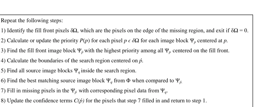
Figure 1: Criminisi's exemplar image completion algorithm Repeat the following steps:

1) Identify the fill front pixels δΩ, which are the pixels on the edge of the missing region, and exit if δΩ = 0.

2) Calculate or update the priority P(p) for each pixel p ϵδΩfor each image block Ψp centered at p.

3) Find the fill front image block Ψṕ with the highest priority among all Ψp centered on the fill front. 4) Find the best matching source image block Ψqfrom Φ when compared to Ψṕ.

5) Fill in missing pixels in the Ψṕ with corresponding pixel data from Ψq.

P(p)=C(p)D(p) ₍₁₎

C(p)=

∑

q∈ Ψp∩(I−Ω)

C(q)

∣Ψp∣

(2)

D(p)=

∣

p⋅np

∣

α (3)

Steps 2 and 4 in Figure 1 are the most important steps in the algorithm. Step 2 determines

the fill order of the missing pixels. The confidence term helps select an image block with the

highest number of known pixel values. The confidence of the image block is basically the

average confidence of all the pixels in the image block. Since the confidence of missing pixels is

0, the confidence of an image block is inversely proportional to the number of missing pixels in

the block. In other words, choosing the image block with the most known pixels is likely to

produce the most reliable pixel values for the missing pixels in that block. Finally, step 6 updates

the confidence of the missing pixels in Ψṕ using the average of the known confidences in Ψṕ.

The data term in step 2 helps the algorithm focus on missing pixels lying on an edge in I.

The data term steers the algorithm to choose edge completion over texture synthesis and thus

create a more visually acceptable output image. The term α is a normalization factor, which is

usually assigned a value of 255 for grayscale images, and np is the unit normal vector with

respect to the fill front. Furthermore, Δ Ip is the isophote that intersects the fill front at point p.

Essentially, the data term calculation steers the filling algorithm based on the direction and

Looking a little deeper into the D(p) calculation, we find that equation (9) requires the

angles of the normal vector and isophote, as well as the magnitude of the isophote. First, create a

mask with the same dimensions as the chosen image block Ψṕ. For each known pixel in Ψṕ set

the corresponding mask value to 1, and similarly, for all the missing pixels in Ψṕ, set the mask

value to 0. The mask essentially imitates the image block Ψṕ with a very strong sharp edge at the

fill front. Then, the algorithm applies an edge filter to the mask values of all the pixels in Ψṕ, and

produces the gradients of the fill front in the x and y directions. Equation (4) uses these gradients

to calculate the angle of np. Next, after applying the same edge filter to the pixel values in Ψṕ,

equations (5) and (6) remove the influence of the fill front to find the true X and Y gradients of

the isophote in the known region of the image block. Obviously, equation (7) applies the

Pythagorean Theorem to the X and Y gradients of the isophote to calculate its magnitude. The

arctan of the isophote gradients gives us the angle of the isophote in equation (8). After the

algorithm performs all the previous calculations, it combines the angles of the isophote and

normal vector and the magnitude of the isophote in the known region of Ψṕ in equation (9) to

find the dot product of the isophote and normal vector.

∢np=arctan(δYconf/δXconf)−π/2 (4)

δXiso=(δXpatch/α)−δXconf (5)

δYiso=(δYpatch/α)−δYconf (6)

∥

∥

√

2 _+δ

Yiso

2 ₎

(7)

D(p)=

∥

∥∥

∥

∥

∥

In step 4 of Figure 1, Criminisi matches image blocks based on the minimum sum of the

squared differences (SSD) of the known pixel values in both image blocks. Therefore, the

algorithm compares the known pixel values of the chosen image block Ψṕ with the

corresponding pixel values in every source image block Ψq.

Some details were not covered in detail in the paper [5] in which Criminisi et al.

presented the algorithm. First, the algorithm only briefly describes which edge detection filter

Criminisi used to find the X and Y gradients when calculating the D(p) for the image block

priority. They used a bidimensional Gaussian kernel but only mentioned that several different

filtering techniques may be employed to complete the data term calculation. In this thesis, a 3×3

Sobel filter [12] was used for the implementation of this algorithm. In addition, Criminisi did not

include a solution for the scenario where more than one Ψq had the same SSD when compared to

Ψṕ. In the implementation of this algorithm used in this thesis, the last image block in the array of

source image blocks with the minimum SSD value was chosen as the match.

Aside from lacking a few minor details, the Criminisi algorithm does its job well but

relatively slowly. In particular, step 4 takes the most time to complete. Comparing the chosen fill

front image block against all of the source image blocks in the image requires a lot of

computations, especially as the size of the image blocks increases. The size of the image block

determines the number of squared differences that need to be calculated for each image block

comparison. However, the benefit of large image block size is a potential reduction in the

iteration. Criminisi set his default image block size to 9×9 pixels. In general, the image block

should be slightly bigger than the largest texel in the image. In addition, the number of source

image blocks for a given image depends on the resolution of the image and the size of the

missing region. Today's culture is moving toward more high definition imagery and Criminisi's

performance suffers at these resolutions.

Overview of Anupam's Algorithm

Anupam [1] makes some specific tweaks to Criminisi's algorithm to improve its accuracy

and speed. Anupam sites Cheng et al. [4] for his accuracy improvements. Cheng et al. [4]

noticed that the confidence term defined in Criminisi's algorithm decreases exponentially. As a

result, they proposed a change to the calculations of the confidence and the priority of an image

block. To combat the adverse effect of the confidence deterioration on the priority, the priority

calculation changed from a product of data and confidence terms to a sum. They regularized the

confidence term in Equation (10) to match it with the order of the data term. In Equation (11),

Cheng adds weights to both confidence and data terms to maintain their balance.

Rc(p)=(1−ω)C(p)+ω,0≤ω≤1 (10)

P(p)=αRc(p)+βD(p), whereα+β=1 (11)

Furthermore, Anupam proposes a solution to one of the problems with Criminisi's

algorithm. Criminisi did not describe what to do if multiple matches are found for the chosen

image block. Anupam's algorithm calculates the variance from the mean of the pixel values

corresponding to the known pixels in the chosen image block. Then, the algorithm chooses the

M=

∑

#{p∣p∈(Φ−Ψ)} (12)

V=

∑

2

# {p∣p∈(Φ−Ψ)} (13)

The final improvement that Anupam proposes is reducing the source area which the

algorithm searches against and thus improving the speed of the algorithm. Assuming that most

matching image blocks can be found in close proximity to the chosen image block, Anupam

creates a bounding box around the chosen image block. Equations (14 - 17) calculate the

boundaries of this search box which is calculated in every iteration of the image completion

algorithm. These equations incorporate the maximum dimensions of the missing region, cr and

cc, so that the bounding box includes some image blocks on all sides of the missing region

corresponding to the chosen image block. The diameter constants Dx and Dy allow the user to

have some control over the size of the search region in both dimensions. The width and height of

an image block are n and m respectively. These equations also check against the input image

boundaries, w and h.

startX=max(0,p−n

2−cr−

Dx

2 ) (14)

startY=max(0,p−m

2−cc−

Dy

2 ) (15)

endX=min(w , p+n

2+cr+

Dx

endY=min(h , p+m

2+cc+

Dy

2 ) (17)

Figure 2: Anupam's image completion algorithm

Anupam addresses some concerns with Criminisi's algorithm in certain scenarios. He

uses variance to break a tie between multiple matching image blocks with the same SSD. In

addition, he tweaks the priority calculations to improve Criminisi's fill order. Anupam's biggest

contribution is eliminating Criminisi's dependence on the input image resolution. Because

Anupams algorithm restricts the source image blocks to a bounding box of a fixed size, step 4

will not take longer to perform for higher resolution images. The number of source blocks is

only dependent on the size of the image block and the maximum size of the missing regions in

the image.

Overview of Kwok’s Exemplar Image Completion with Fast Query Algorithm

Kwok's algorithm [13] is also based on Criminisi's algorithm [5]. The goal of this

algorithm is real-time image editing. Kwok focused on optimizing the image block matching step

4 in Criminisi's algorithm. Instead of comparing pixel values to find a match, Kwok transforms

Repeat the following steps:

1) Identify the fill front pixels δΩ, which are the pixels on the edge of the missing region, and exit if δΩ = 0. 2) Calculate or update the priority P(p) for each pixel p ϵδΩfor each image block Ψp centered at p.

3) Find the fill front image block Ψṕ with the highest priority among all Ψp centered on the fill front. 4) Calculate the boundaries of the search region centered on ṕ.

5) Find all source image blocks Ψq inside the search region.

6) Find the best matching source image block Ψqfrom Φ when compared to Ψ_ṕ. 7) Fill in missing pixels in the Ψṕ with corresponding pixel data from Ψq.

each image block into the frequency domain using a discrete cosine transform (DCT) and

compares a fraction of the DCT coefficients. In doing so, Kwok drastically reduces the number

of calculations done for each source image block comparison. The top 0.1 % of source image

blocks that match in the frequency domain are then compared using the SSD of pixel values to

find the best matching source image block.

Figure 3: Kwok's image completion algorithm

Kwok had to perform a few more tweaks to get this algorithm working properly. The

method for choosing the DCT coefficients for comparison needed to be considered. Choosing

the coefficients associated with the m lower frequencies from the upper left corner of the block

does not work for highly textured images. When comparing images based on DCT coefficients,

images with similar energy levels at the same frequencies tend to be better matches. Thus, Kwok

found that using the m most significant coefficients, in terms of their energy, worked best.

Furthermore, in order to preserve the continuity of image information when calculating

the DCT of image blocks with missing pixels, the missing pixels needed to be filled in with a

local gradient. Using the average pixel value of the image block did not create the proper DCT

Repeat the following steps:

1) Identify the fill front pixels δΩ, which are the pixels on the edge of the missing region, and exit if δΩ=0.

2) Calculate or update the priority P(p) for each pixel p ϵδΩfor each image block Ψp centered at p.

3) Find the fill front image block Ψ_ṕ with the highest priority among all Ψp centered on the fill front. 4) Fill in missing pixels of Ψṕwith gradient.

5) Find m truncated DCT coefficients of Ψ_ṕ.

6) Find the 0.1% source image blocks Ψqfrom Φ with the lowest scores using Kwok’s fast query algorithm.

7) Compare known pixel values of Ψṕwith the Ψq found in step 6.

coefficients and, subsequently, poor matches. To find the pixel values for the gradient, the

algorithm must solve an overdetermined system of linear equations. For each missing pixel pi,j ,

let

pi−1,j−pi , j=0 (18)

pi , j−1−pi , j=0 (19)

Therefore, each missing pixel generates 2 equations with its left and top neighbors.

Kwok employed the Least Squares Solution to solve this system of equations and minimize the

norm of gradients at the missing pixels. Equation (20) shows the matrix form of the Least

Squares solution. The vector C contains a list of the unknown and known pixels involved in the

system of equations. The Y vector contains a 0 for each row in X that corresponds to either

equation (18) or (19). The other elements in Y are the pixel values of the known pixels. The rows

in X corresponding to the known pixels simply consist of a 1 at the position of the known pixel in

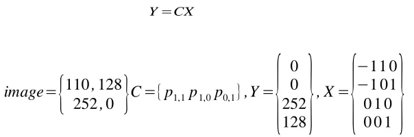
C and the rest of the elements in the row are 0. Figure 4 shows an example of the least squares

calculation. I used the GNU Scientific Library to provide the Least Squares calculations for the

gradient filling algorithm.

Y=CX ₍₂₀₎

image=

{

252,0

}

{

}

, X=

{

−1 01 0 1 0 0 0 1

}

Kwok further reduced the calculations required for comparing DCT coefficients. The

square of the differences of the coefficients in equation (21) becomes equation (23). The base

score of the chosen block dp is constant for all the comparisons and thus, can be ignored in

equation (22). Moreover, the base score dqcan be calculated for the source blocks in the

initialization step before the loop starts. This leaves only dpq to be calculated during the

comparison step of each iteration of the main loop. Originally, the algorithm would do n2

multiplications and n2 subtractions. After some simple algebra is applied, the number of

calculations decreases to 2m+1 multiplications and 1 subtraction.

d(Ψ_p,Ψ_q)=

∑

(i , j)

( ̂p_{i , j}−̂q_{i , j})2=

∑

(i , j)

( ̂p_{i , j}−̂q_{i , j})( ̂p_{i , j}− ̂q_{i , j})

(21)

d(Ψp,Ψq)=dp+dq−2dpq

where , dp=

∑

̂

pi, j≠0

( ̂pi , j)

2

dq=

∑

̂

qi , j≠0

( ̂qi , j)

2

dpq=

∑

̂

p_{i , j}≠0,q̂_{i , j}≠0

̂ pi , jq̂i , j

(22)

S(Ψp,Ψq)=dq−2dpq (23)

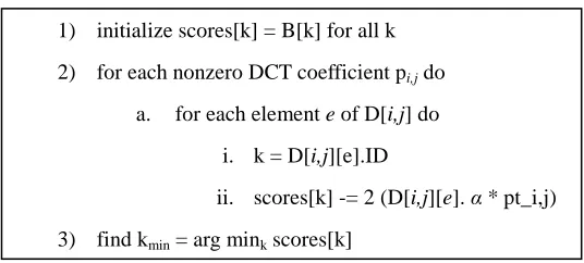
Kwok additionally improves performance by developing a fast image query algorithm.

During initialization, Kwok's algorithm creates several arrays to be used during the search for a

match. All of the source blocks are transformed by the DCT and the coefficients are truncated

until only m coefficients remain. Then, the base scores dq are calculated and stored in a base

score array B, where B[k] is the base score of the kth source block. The non-zero m coefficients

where (i,j) corresponds to the position of the DCT coefficient within the transform. The term k

refers to a source block with a non-zero coefficient at (i,j). Every element of the search-array

contains the global ID of the source block with a coefficient and the value α of that coefficient.

The following fast query algorithm uses these arrays and the m significant coefficients of the

chosen image block to find matching source blocks. The algorithm selects 0.1% of source blocks

with the lowest scores to be matched using the traditional SSD of pixel values as Criminisi did in

his algorithm.

Figure 5: Kwok's Fast Query Algorithm

By performing most of the calculations in parallel on a modern GPU, Kwok was able to

increase the algorithm’s operations per second and minimize its run-time. Parallelization was not

included in the implementation of Kwok's algorithm used in this thesis.

Overview of Proposed Algorithm

The proposed work combines Anupam's algorithm and Kwok's algorithm. More

specifically, Anupam's bounding box was applied to Kwok's DCT-based fast query algorithm.

Instead of creating the search array before the loop begins, the proposed implementation

reinitializes the search array structure on every iteration of the main loop. However, the search

array only includes the transform coefficients from the source blocks that exist within the

1) initialize scores[k] = B[k] for all k

2) for each nonzero DCT coefficient pi,j do

a. for each element e of D[i,j] do

i. k = D[i,j][e].ID

ii. scores[k] -= 2 (D[i,j][e]. α * pt_i,j)

bounding box limits defined in Anupam's work. Furthermore, the DCT coefficients and

basescore dq of each source block is only calculated once and saved when the fast query

algorithm compares it for the first time. They are not calculated during initialization which

speeds that portion of the algorithm up. No time is wasted calculating transformations and

basescores for source blocks that are never used.

This additional spatial restriction increases the efficiency of Kwok's fast query algorithm

when searching for the matching source block. In most cases, far less coefficients need to be

compared in the search array. Furthermore, once the DCT matches are found, no time will be

wasted comparing the source blocks far away from the chosen block using traditional SSD

calculations.

Results and Discussion

All of the algorithms were implemented in the C programming language and compiled

with the GCC compiler. The computer used for testing was a Thinkpad R60 with an Intel Core 2

Duo running at 1.8GHz and 4 GB of ram. The laptop was running Ubuntu 10.04 64-bit for the

Operating System. Furthermore, two open source libraries were used to aid in the

implementations. The FreeImage C/C++ library [6] was used for loading, manipulating, and

saving bitmap images in all of the algorithms discussed in this paper. In addition, the GNU

Scientific Library [9] was used to calculate the least-squares approximation in Kwok's gradient

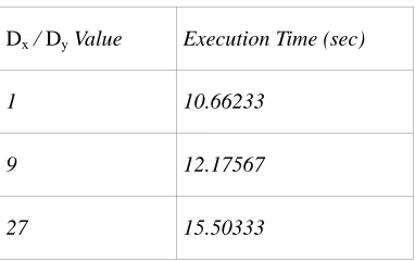
Dx / Dy Value Execution Time (sec)

1 10.66233

9 12.17567

27 15.50333

Table 1: Timed execution comparison in seconds of Anupam's algorithm with different values for Dx and Dy.

Figure 6: Input images used in the comparisons. Missing Regions are shown in black patches. From left to right the images are: chimney, Lena Wall, Lena Hat, simple, and bricks.

(a) (b) (c)

Figure 7: Visual Quality comparison of Anupam's outputs with different values of Dx and Dy using Lena all image..

From left to right: Dx = Dy = 1, Dx = Dy = 9, and Dx = Dy = 27.

First, Anupam’s work and Kwok’s work both glance over some important variables in

their algorithms. Anupam's bounding box calculation includes two constants Dx and Dy. Anupam

expand the search area used to find matches in all four directions. Figure 7 shows the output of

Anupam's algorithm with several different values of Dx and Dy. The images in Figure 7 look

almost identical because the smallest bounding box was sufficient to fill in the missing region.

Some images may need this value enlarged to find better matches and enhance the visual quality

of the output image. Thus, the user should be able to adjust these constants to accommodate

different input images. Additionally, the execution times are listed in Table 1. As a result of

increasing the bounding box size, the algorithm must perform more comparisons during every

iteration of the main loop, which, in turn, increases execution time. However, the algorithm

scales well with these constants. The constants increased 2700% but the execution time only

increased 50%.

m Execution Time (seconds)

4 (5%) 108.5617

8 (10%) 123.999

40 (50%) 305.869

Table 2: Execution time comparison for Kwok's algorithm with different numbers of truncated coefficients.

Furthermore, the efficiency of Kwok's algorithm is based on truncating the DCT

coefficients of the image block down to m significant coefficients. Kwok’s original work [13]

never mentions a default value for m. In Figure 8, the visual results for several different values

of m are shown. Since the number of coefficients change with the size of the image block, the

algorithm uses a certain percentage of the total coefficients calculated by the DCT. For Figure 8

and Table 2, the image block size was 9×9 pixels. Thus, the values of m correspond to 5%, 10%,

and 50% of the total coefficients. The best looking output in Figure 8 is m = 8. Theoretically,

However, the output image for m = 40 is less visually appealing than the output image produced

for m = 8. Part of the reason is error propagation. Since the image block is relatively small,

when compared to the resolution of the input image, and the edge in the missing region is not

well defined, very little pixel value change occurs within a given block. As a result, two

different image blocks with very different pixel values may have similar DCT coefficients.

Consequently, most of the transforms have similar values, and comparing more coefficients

could cause a matching error. In addition, the execution times for different values of m are

displayed in Table 2. Increasing the number of truncated coefficients gives the algorithm more

calculations for each image block comparison. Therefore, the execution time will suffer for

higher values of m. The best scenario would be to let the user adjust the value of m to achieve the

best combination of performance and visual quality.

(a) (b) (c)

Figure 8: Visual Quality Comparison using Lens Wall image of Kwok's algorithm with different numbers of truncated coefficients. From left to right: m = 4, m = 8, and m = 40

Next, some interesting performance results for all four algorithms across multiple images

are displayed in Table 3. In general, Kwok’s algorithm is slightly slower than Criminisi’s

overhead of DCT transformations in our single-threaded implementation of Kwok’s algorithm

and the proposed algorithm outweighs the computational efficiency of comparing a small subset

of DCT coefficients. DCT transformations and the fast query algorithm developed by Kwok

allow for easy parallelization. Thus, Kwok implemented his algorithm in parallel on a GPU,

which significantly reduced the execution time of the algorithm. The proposed algorithm suffers

from the same single-threaded performance issues in our implementation.

Image Size (pixels) % Missing Execution Time (in seconds)

Criminisi Anupam Kwok Contribution

simple 16384 6.99 1.006 0.557 1.96 1.548

bricks 22500 14.89 3.273 7.834 4.374 10.79

chimney 196608 2.49 38.164 4.069 54.352 12.807

Lena wall 262144 2.37 83.724 12.176 123.999 27.59

Lena hat 262144 1.62 42.534 4.828 75.815 14.042

Table 3: Execution time of all four algorithms across different images.

Figure 9: Visual comparison of simple image across all four algorithms. From left to right: Criminisi, Anupam, Kwok, and the proposed algorithm.

Anupam's algorithm is the fastest of the four algorithms in most cases. The exception to

this observation was the bricks image. The relatively large missing region pushes the size of the

bounding box region to almost equal the size of the actual image. In this case, the bounding box

boundaries and discovering the source image blocks on every iteration of the main loop.

Consequently, when compared to Criminisi’s algorithm, Anupam’s algorithm does extra work

without any computational efficiency benefits in this scenario. For the same reason, the

proposed algorithm performs poorly on the bricks image when compared to Kwok’s algorithm.

For some users, the visual quality of the outputs of these four algorithms is the

most important consideration. The visual results in Figure 9 show the difference between pixel

value matching and DCT coefficient matching. Criminisi’s algorithm and Anupam’s algorithm

use pixel value matching and achieve better results than the other two algorithms. DCT

matching may choose source image blocks similar to the chosen image block but does not

always choose the best visual match. The chimney image in Figure 10 shows that all four

algorithms can concurrently manage more than one missing region in the input image.

Considering the missing region on the roof, Criminisi’s algortihm and Anupam’s algorithm have

better quality output images. Once again, the algorithms using DCT matching fail to produce

better visual results. The proposed method has the worst output on the roof. A combination of

its small search region and DCT coefficient matching is to blame. The missing chimney region

in Figure 10 is a little more interesting. None of the algorithms reconstructed the brick layout

perfectly. Anupam’s algorithm has the best output because its small search area helps it focus on

the middle of the chimney, where the best matching image blocks exist. On the other hand,

Criminisi’s algorithm searches over the whole image and chooses a few images blocks from

bricks that touch parts of the flashing around the chimney. As a result, Criminisi’s algorithm

produces a result with some major visual imperfections. Kwok’s algorithm and the proposed

truncation in both algorithms. Because of the truncation, image blocks with very little edge

information were chosen, which broke the brick layout pattern. Again the small search area

seems to improve the output of the proposed solution compared to Kwok’s algorithm. Figure 11

further reinforces these observations on the Lena wall image.

(a) (b)

(c) (d)

(a) (b)

(c) (d)

Figure 11: Visual comparison of Lena wall image across all four algorithms. Criminisi (a), Anupam (b), Kwok (c), and the proposed algorithm (d).

The synthetic brick pattern in the brick image in Figure 12 demonstrates two different

issues possible in all four algorithms. The Criminisi algorithm’s output shows overshooting.

Overshooting occurs when the algorithm does not know when an edge should terminate in the

image. Thus, the edge in the algorithm’s output image extends further than it should. Figure 14

gives a simpler example of overshooting at the corner of an object. The results in Figure 12 for

Kwok and the proposed algorithm demonstrate error propagation. The white lines between the

with lines in them during a certain iteration of the loop. Subsequent iterations based their

matches on the poor match that came before them. As a result, a single matching error snowballs

into many errors in the output image. An additional example of this issue is observed in Figure

15.

(a) (b) (c) (d)

(a) (b)

(c) (d)

Figure 13: Visual comparison of Lena hat image across all four algorithms: Criminisi (a), Anupam (b), Kwok (c), and the proposed algorithm (d).

Figure 14: An Example of overshooting. Input image on the left and the output image from the proposed algorithm on the right.

Figure 15: Example of error propagation. Input image on the left and result of Anupam's Algorithm on the right

Conclusion

Each of these four algorithms has its own strengths and weaknesses. Criminisi’s

algorithm’s pixel value matching allows it to produce decent results on any image. However, the

user may need to adjust the block size used in searching to reduce the effects of error propagation

and overshooting. In addition, Criminisi’s algorithm is relatively slow and would not be a good

On the other hand, Anupam’s algorithm’s spatial restriction can significantly improve its

performance. Unfortunately, a weakness of the spatial restriction is poor performance for large

missing regions. In addition, Anupam’s algorithm creates the best visual results in most of the

figures in this thesis. However, certain input images may require a larger search region to

produce the best visual results. Moreover, Anupam’s algorithm has several more parameters than

Criminisi and Kwok, which can be adjusted to achieve a better balance between performance and

visual quality.

Kwok’s algorithm consistently is the slowest of the four algorithms in the results.

However, Kwok’s biggest strength is its ability to be parallelized. The efficiency of the

algorithm could improve significantly if the algorithm performs the DCT transformations in

parallel. Although the results for Kwok are not the best, adjusting block size and m can improve

the visual output. Furthermore, error propagation and overshooting are possible in Kwok’s

algorithm.

The proposed algorithm inherits the strengths and weaknesses of all three other

algorithms. First, the spatial restrictions of Anupam’s algorithm help the proposed algorithm

perform better than Kwok and Criminisi. However, similar to Anupam’s algoritm, large missing

regions hinder the performance of the proposed algorithm. In addition, the proposed algorithm

can be easily parallelized just like Kwok’s, which could make it faster than Anupam’s algorithm

in some cases. The visual quality of the results is on par with that of Kwok’s algorithm. Error

propagation and overshooting are possible in the proposed algorithm as well. Finally, the

proposed algorithm has the most parameters which the user can adjust to achieve the best

Bibliography

[1] Anupam, Goyal, P., & Diwakar, S. (2010). Fast and Enhanced Algorithm for Exemplar

Based Image Inpainting. Fourth Pacific-Rim Symposium on Image and Video Technology,

(pp. 325-330).

[2] Bertalmio, M., Bertozzi, A., & Sapiro, G. (2001). Navier-stokes, fluid dynamics, and

image and video inpainting. Proceedings of the 2001 IEEE Computer Society Conference

on Computer Vision and Pattern Recognition, 1, pp. I-355- I-362.

[3] Bertalmio, M., Vese, L., Sapiro, G., & Osher, S. (2003). Simultaneous structure and

texture image inpainting. IEEE Computer Society Conference on Computer Vision and

Pattern Recognition, 2, pp. II- 707-12.

[4] Cheng, W.-H., Hsieh, C.-W., Lin, S.-K., Wang, C.-W., & Wu, J.-L. (2005). Robust

Algorithm for Exemplar-Based Image Inpainting. The International Conference on

Computer Graphics, Imaging and Vision, (pp. 64-69).

[5] Criminisi, A., Perez, P., & Toyama, K. (2004). "Region filling and object removal by

exemplar-based image inpainting,". IEEE Transactions on Image Processing, 13,

1200-1212.

[6] Drolon, H. R. (n.d.). The FreeImage Project, 3.15.0. Retrieved January 2, 2011, from

http://freeimage.sourceforge.net

[7] Efros, A., & Leung, T. (2009). Texture synthesis by non-parametric sampling. The

Proceedings of the Seventh IEEE International Conference on Computer Vision, 2, pp. 1033-1038.

[8] Fang, C.-W., & Lien, J.-J. (2009, Dec.). "Rapid Image Completion System Using

Multiresolution Patch-Based Directional and Nondirectional Approaches,". IEEE

Transactions on Image Processing, 18, pp. 2769-2779.

[9] GNU Scientific Library. (n.d.). Retrieved March 1, 2011, from

http://www.gnu.org/software/gsl/

[10] I. Drori, D. C.-O. (2003). Fragment-based image completion. ACM Trans. Graph., 22,

303–312.

[11] Jacobs, C. E., Finkelstein, A., & Salesin, D. H. (1995). Fast multiresolution image

querying. Proc. 22nd Ann. Conf. Comput. Graph. Interactive Techniques, (pp. 277–286).

[12] Kuo, C.-M., Yang, N.-C., Chang, W.-H., & Wu, C.-L. (2008). "Image Recovery Based on

Effective Image Completion". IIHMSP '08 International Conference on Intelligent

Information Hiding and Multimedia Signal Processing, (pp. 393-396).

[13] Kwok, T.-H., Sheung, H., & Wang, C. (2010). Fast Query for Exemplar-Based Image

Completion. IEEE Transactions on Image Processing, 19 (12), 3106-3115.

[14] Levin, A., Zomet, A., & Weiss, Y. (2003). Learning how to inpaint from global image

statistics. Proceedings. Ninth IEEE International Conference on Computer Vision, (pp.

305-312).

[15] Mobahi, H., Rao, S., & Ma, Y. (2009). "Data-driven image completion by image patch

subspaces". Picture Coding Symposium, (pp. 1-4,6-8).

[16] Orii, H., Kawano, H., Maeda, H., & Ikoma, N. (2009). "Image completion with

Vita

The author was born in Metairie, Louisiana. He obtained his Bachelor's degree from Louisiana

State University in 2003. He joined the University of New Orleans graduate program to pursue a