A Robust Learning Approach for Regression Models Based on Distributionally Robust Optimization

(1)

A Robust Learning Approach for Regression Models Based

on Distributionally Robust Optimization

Ruidi Chen [email protected]

Division of Systems Engineering, Boston University,

Boston, MA 02215, USA

Ioannis Ch. Paschalidis [email protected]

Department of Electrical and Computer Engineering, Division of Systems Engineering,

and Department of Biomedical Engineering, Boston University,

Boston, MA 02215, USA sites. bu. edu/ paschalidis

Editor:Edo Airoldi

Abstract

We present aDistributionally Robust Optimization (DRO)approach to estimate a robusti-fied regression plane in a linear regression setting, when the observed samples are potentially contaminated with adversarially corrupted outliers. Our approach mitigates the impact of outliers by hedging against a family of probability distributions on the observed data, some of which assign very low probabilities to the outliers. The set of distributions under con-sideration are close to the empirical distribution in the sense of the Wasserstein metric. We show that this DRO formulation can be relaxed to a convex optimization problem which encompasses a class of models. By selecting proper norm spaces for the Wasserstein metric, we are able to recover several commonly used regularized regression models. We provide new insights into the regularization term and give guidance on the selection of the regularization coefficient from the standpoint of a confidence region. We establish two types of performance guarantees for the solution to our formulation under mild conditions. One is related to its out-of-sample behavior (prediction bias), and the other concerns the discrepancy between the estimated and true regression planes (estimation bias). Extensive numerical results demonstrate the superiority of our approach to a host of regression mod-els, in terms of the prediction and estimation accuracies. We also consider the application of our robust learning procedure to outlier detection, and show that our approach achieves a much higher AUC (Area Under the ROC Curve) than M-estimation (Huber, 1964, 1973).

Keywords: Robust Learning, Distributionally Robust Optimization, Wasserstein Metric, Regularized Regression, Generalization Guarantees.

1. Introduction

Consider a linear regression model with responsey ∈R, predictor vectorx∈Rm−1,

regres-sion coefficientβ∗ ∈_Rm−1 _{and error} _∈

R:

y=x0β∗+.

c

(2)

Given samples (xi, yi), i = 1, . . . , N, we are interested in estimating β∗. The Ordinary

Least Squares (OLS) minimizes the sum of squared residuals PN

i=1(yi−x

0

iβ)2, and works

well if all the N samples are generated from the underlying true model. However, when faced with adversarial perturbations in the training data, the OLS estimator will deviate from the true regression plane to reduce large residuals. Alternatively, one can choose to minimize the sum of absolute residualsPN

i=1|yi−x0iβ|, as done inLeast Absolute Deviation

(LAD), to mitigate the influence of large residuals. Another commonly used approach for

hedging against outliers is M-estimation (Huber, 1964, 1973), which minimizes a symmetric loss function ρ(·) of the residuals in the form PN

i=1ρ(yi −x

0

iβ), which downweights the

influence of samples with large absolute residuals. Several choices forρ(·) include the Huber function (Huber, 1964, 1973), the Tukey’s Biweight function (Rousseeuw and Leroy, 2005), the logistic function (Coleman et al., 1980), the Talwar function (Hinich and Talwar, 1975), and the Fair function (Fair, 1974).

Both LAD and M-estimation are not resistant to large deviations in the predictors. For contamination present in the predictor space, high breakdown value methods are required. Examples include theLeast Median of Squares (LMS)(Rousseeuw, 1984), which minimizes the median of the absolute residuals, theLeast Trimmed Squares (LTS)(Rousseeuw, 1985), which minimizes the sum of theq smallest squared residuals, and S-estimation (Rousseeuw and Yohai, 1984), which has a higher statistical efficiency than LTS with the same break-down value. A combination of the high breakbreak-down value method and M-estimation is the MM-estimation (Yohai, 1987). It has a higher statistical efficiency than S-estimation. We refer the reader to the book of Rousseeuw and Leroy (2005) for a detailed description of these robust regression methods.

(3)

The existing literature on DRO can be split into two main branches according to the way in which P is defined. One is through a moment ambiguity set, which contains all distributions that satisfy certain moment constraints (see Popescu, 2007; Delage and Ye, 2010; Goh and Sim, 2010; Zymler et al., 2013; Wiesemann et al., 2014). In many cases, it leads to a tractable DRO problem but has been criticized for yielding overly conservative solutions (Wang et al., 2016). The other is to defineP as a ball of distributions using some probabilistic distance functions such as theφ-divergences (Bayraksan and Love, 2015), which include the Kullback-Leibler (KL) divergence (Hu and Hong, 2013; Jiang and Guan, 2015) as a special case, the Prokhorov metric (Erdo˘gan and Iyengar, 2006), and the Wasserstein distance (Esfahani and Kuhn, 2015; Gao and Kleywegt, 2016; Zhao and Guan, 2015; Luo and Mehrotra, 2017; Blanchet and Murthy, 2016). Deviating from the stochastic setting, there are also some works focusing on deterministic robustness. El Ghaoui and Lebret (1997) consider the least squares problem with unknown but bounded, non-random disturbance and solve it in polynomial time. Xu et al. (2010) study the robust linear regression problem with norm-bounded feature perturbation and show that it is equivalent to the`1-regularized regression. See Yang and Xu (2013); Bertsimas and Copenhaver (2017) which also use a deterministic robustness approach.

In this paper we consider a DRO problem withP containing distributions that are close to the discrete empirical distribution in the sense of Wasserstein distance. The reason for choosing the Wasserstein metric is two-fold. On one hand, the Wasserstein ambiguity set is rich enough to contain both continuous and discrete relevant distributions, while other metrics such as the KL divergence, exclude all continuous distributions if the nominal dis-tribution is discrete (Esfahani and Kuhn, 2015; Gao and Kleywegt, 2016). Furthermore, considering distributions within a KL distance from the empirical, does not allow for prob-ability mass outside the support of the empirical distribution. On the other hand, measure concentration results guarantee that the Wasserstein set contains the true data-generating distribution with high confidence for a sufficiently large sample size (Fournier and Guillin, 2015). Moreover, the Wasserstein metric takes into account the closeness between sup-port points while other metrics such as the φ-divergence only consider the probabilities of these points. The image retrieval example in Gao and Kleywegt (2016) suggests that the probabilistic ambiguity set constructed based on the KL divergence prefers the pathologi-cal distribution to the true distribution, whereas the Wasserstein distance does not exhibit such a problem. The reason lies in thatφ-divergence does not incorporate a notion of close-ness between two points, which in the context of image retrieval represents the perceptual similarity in color.

Our DRO problem minimizes the worst-case absolute residual over a Wasserstein ball of distributions, and could be relaxed to the following form:

inf

β

1

N

X

i=1

|yi−x0iβ|+k(−β,1)k∗, (1)

where is the radius of the Wasserstein ball, and k · k∗ is the dual norm of the norm

(4)

simply reduces to regularized regression models, we want to emphasize a few new insights brought by this methodology. First, the regularization term controls the conservativeness of the Wasserstein set, or the amount of ambiguity in the data, which differentiates itself from the heuristically added regularizers in traditional regression models that serve the purpose of preventing overfitting, error/variance reduction, or sparsity recovery. Second, the regularization term is determined by the dual norm of the regression coefficient, which controls thegrowth rateof the `1-loss function, and the radius of the Wasserstein set. This

connection provides guidance on the selection of the regularization coefficient and may lead to significant computational savings compared to cross-validation. DRO essentially enables new and more accurate interpretations of the regularizer, and establishes its dependence on

the growth rate of the loss, the underlying metric space and the reliability of the observed

samples.

The connection between robustness and regularization has been established in several works. The earliest one may be credited to El Ghaoui and Lebret (1997), who show that minimizing the worst-case squared residual within a Frobenius norm-based perturbation set is equivalent to Tikhonov regularization. In more recent works, using properly selected uncertainty sets, Xu et al. (2010) have shown the equivalence between robust linear regres-sion with feature perturbations and the Least Absolute Shrinkage and Selection Operator

(LASSO). Yang and Xu (2013) extend this to more general LASSO-like procedures,

includ-ing versions of the grouped LASSO. Bertsimas and Copenhaver (2017) give a comprehensive characterization of the conditions under which robustification and regularization are equiv-alent for regression models with deterministic norm-bounded perturbations on the features. For classification problems, Xu et al. (2009) show the equivalence between the regularized Support Vector Machines (SVMs) and a robust optimization formulation, by allowing poten-tially correlated disturbances in the covariates. Shafieezadeh-Abadeh et al. (2015) consider a robust version of logistic regression under the assumption that the probability distributions under consideration lie in a Wasserstein ball, and they show that the regularized logistic regression is a special case of this robust formulation. Recently, Shafieezadeh-Abadeh et al. (2017); Gao et al. (2017) have provided a unified framework for connecting the Wasserstein DRO with regularized learning procedures, for various regression and classification models. Our work is motivated by the problem of identifying patients who receive an abnormally high radiation exposure in CT exams, given the patient characteristics and exam-related variables (Chen et al., 2018). This could be casted as an outlier detection problem; specifi-cally, estimating a robustified regression plane that is immunized against outliers and learns the underlying true relationship between radiation dose and the relevant predictors. We focus on robust learning of the parameter in regression models under distributional per-turbations residing within a Wasserstein ball. While the applicability of the Wasserstein DRO methodology is not restricted to regression analysis (Sinha et al., 2017; Gao et al., 2017; Shafieezadeh-Abadeh et al., 2017), or a particular form of the loss function (as long as it satisfies certain smoothness conditions (Gao et al., 2017)), we focus on the absolute residual loss in linear regression in light of our motivating application and for the purpose of enhancing robustness. Our contributions can be summarized as follows:

1. We develop a DRO approach to robustify linear regression using an `1 loss

(5)

in-clude any norm-induced Wasserstein metric and incorporate additional regularization constraints on the regression coefficients (e.g., `1-norm constraints). It provides an intuitive connection between the amount of ambiguity allowed and a regularization penalty term in the robust formulation, which provides a natural way to adjust the latter.

2. We establish novel performance guarantees on both the out-of-sample loss (prediction bias) and the discrepancy between the estimated and the true regression coefficients (estimation bias). Our guarantees elucidate the role of the regularizer, which is related to the dual norm of the regression coefficients, in bounding the biases and are in concert with the theoretical foundation that leads to the regularized problem. The generalization error bound, in particular, builds a connection between the loss function and the form of the regularizer via Rademacher complexity, providing a rigorous explanation for the commonly observed good out-of-sample performance of regularized regression. On the other hand, the estimation error bound corroborates the validity of the`1-loss function, which tends to incur a lower estimation bias than other candidates such as the `2 and `∞ losses. Our results are novel in the robust regression setting

and different from earlier work in the DRO literature, enabling new perspectives and interpretations of the norm-based regularization, and providing justifications for the

`1-loss-based learning algorithms.

3. We empirically explore three important aspects of the Wasserstein DRO formulation, including the advantages of the`1-loss function, the selection of a proper norm for the

Wasserstein metric, and the implication of penalizing the extended regression

coeffi-cient(−β,1), by comparing with a series of regression models on a number of synthetic

datasets. We show the superiority of the Wasserstein DRO approach, presenting a thorough analysis under four different experimental setups. We also consider the ap-plication of our methodology to outlier detection and compare with M-estimation in terms of the ability of identifying outliers (ROC (Receiver Operating Characteristic)

curves). The Wasserstein DRO formulation achieves significantly higher AUC (Area

Under Curve) values.

The rest of the paper is organized as follows. In Section 2, we introduce the Wasserstein metric and derive the general Wasserstein DRO formulation in a linear regression framework. Section 3 establishes performance guarantees for both the general formulation and the special case where the Wasserstein metric is defined on the `1-norm space. Numerical

experimental results are presented in Section 4. We conclude the paper in Section 5.

Notational conventions: We use boldfaced lowercase letters to denote vectors, or-dinary lowercase letters to denote scalars, boldfaced uppercase letters to denote matri-ces, and calligraphic capital letters to denote sets. E denotes expectation and P

proba-bility of an event. All vectors are column vectors. For space saving reasons, we write

x = (x1, . . . , xdim(x)) to denote the column vector x, where dim(x) is the dimension of x.

We use prime to denote the transpose of a vector,k · kfor the general norm operator, k · k2

for the `2 norm, k · k1 for the`1 norm, andk · k∞ for the infinity norm. P(Z) denotes the

set of probability measures supported on Z. ei denotes the i-th unit vector, ethe vector

(6)

norm k · k∗ is defined as: kθk∗ , supkzk≤1θ0z. For a function h(z), its convex conjugate h∗(·) is defined as: h∗(θ) ,sup_z∈dom h {θ0z−h(z)},where dom h denotes the domain of

the functionh.

2. Problem Statement and Justification of Our Formulation

Consider a linear regression problem where we are given a predictor/feature vector x ∈

Rm−1, and a response variable y ∈ R. Our goal is to obtain an accurate estimate of the

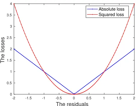
regression plane that is robust with respect to the adversarial perturbations in the data. We consider an`1-loss functionhβ(x, y),|y−x0β|, motivated by the observation that the

absolute loss function is more robust to large residuals than the squared loss (see Fig. 1). Moreover, the estimation error analysis presented in Section 3.2 suggests that the `1-loss function leads to a smaller estimation bias than others. Our Wasserstein DRO problem using the`1-loss function is formulated as:

inf

β∈B_Qsup_∈_ΩE

Q

|y−x0β|

, (2)

whereβis the regression coefficient vector that belongs to some setB. Bcould beRm−1, or

B={β :kβk1 ≤l} if we wish to induce sparsity, withl being some pre-specified number.

Qis the probability distribution of (x, y), belonging to some set Ω which is defined as:

Ω,{_Q∈ P(Z) :Wp(Q, PˆN)≤},

where Z is the set of possible values for (x, y); P(Z) is the space of all probability distri-butions supported onZ;is a pre-specified radius of the Wasserstein ball; and Wp(Q, ˆPN)

is the order-p Wasserstein distance between Qand ˆPN (see definition in (3)), with ˆPN the

uniform empirical distribution over samples. The formulation in (2) is robust since it mini-mizes over the regression coefficients the worst case expected loss, that is, the expected loss maximized over all probability distributions in the ambiguity set Ω.

Before deriving a tractable reformulation for (2), let us first define the Wasserstein metric. Let (Z, s) be a metric space whereZis a set andsis a metric onZ. The Wasserstein metric of orderp≥1 defines the distance between two probability distributionsQ1 andQ2

in the following way:

Wp(Q1,Q2), min Π∈P(Z×Z)

Z

Z×Z

s((x1, y1),(x2, y2)) p

Π d(x1, y1), d(x2, y2)

!1/p , (3)

where Π is the joint distribution of (x1, y1) and (x2, y2) with marginalsQ1 and Q2,

respec-tively. The Wasserstein distance betweenQ1and Q2 represents the cost of an optimal mass

transportation plan, where the cost is measured through the metric s. The order p should be selected in such a way as to ensure that the worst-case expected loss is meaningfully defined, i.e.,

EQhβ(x, y)

<∞, ∀Q∈Ω. (4)

Notice that the ambiguity set Ω is centered at the empirical distribution ˆPN and has radius

. It may be desirable to translate (4) into:

E

Q

hβ(x, y)

−EPˆNhβ(x, y)

(7)

-2 -1.5 -1 -0.5 0 0.5 1 1.5 2

The residuals

0 0.5 1 1.5 2 2.5 3 3.5 4

The losses

Absolute loss Squared loss

Figure 1: Comparison between `1 and`2 loss functions.

We want to relate (5) with the Wasserstein distanceWp(Q, ˆPN), which is no larger than

for all Q∈Ω. The LHS of (5) could be written as:

E

Q

hβ(x, y)

−EPˆNhβ(x, y)

=

Z

hβ(x1, y1)Q(d(x1, y1))− Z

Z

hβ(x2, y2)ˆPN(d(x2, y2))

=

Z

hβ(x1, y1) Z

Z

Π0(d(x1, y1), d(x2, y2))− Z

Z

hβ(x2, y2) Z

Z

Π0(d(x1, y1), d(x2, y2))

≤

Z

Z×Z

h_β(x₁, y₁)−h_β(x₂, y₂)

Π₀(d(x₁, y₁), d(x₂, y₂)),

(6)

where Π0 is the joint distribution of (x1, y1) and (x2, y2) with marginalsQand ˆPN,

respec-tively. Comparing (6) with (3), we see that for (5) to hold, the following quantity which characterizes thegrowth rate of the loss function needs to be bounded:

GRhβ((x1, y1),(x2, y2)),

h_β(x₁, y₁)−h_β(x₂, y₂)

s((x1, y1),(x2, y2))p , ∀(x1, y1),(x2, y2)∈ Z. (7)

A formal definition of the growth rate is due to Gao and Kleywegt (2016), which takes the limit of (7) as s((x1, y1),(x2, y2)) → ∞, to eliminate its dependence on (x, y). One important aspect they have pointed out is that when the growth rate of the loss function is infinite, strong duality for the worst-case problem sup_Q∈ΩEQ

hβ(x, y)

(8)

induced by some normk · k, the boundedgrowth raterequirement is expressed as follows:

lim sup

k(x1,y1)−(x2,y2)k→∞

|hβ(x1, y1)−hβ(x2, y2)|

k(x1, y1)−(x2, y2)kp

≤ lim sup

k(x1,y1)−(x2,y2)k→∞

|y1−x0₁β−(y2−x0₂β)|

k(x1, y1)−(x2, y2)kp

≤ lim sup

k(x1,y1)−(x2,y2)k→∞

k(x1, y1)−(x2, y2)kk(−β,1)k∗

k(x1, y1)−(x2, y2)kp <∞,

(8)

wherek · k∗ is the dual norm ofk · k, and the second inequality is due to the Cauchy-Schwarz

inequality. Notice that by taking p = 1, (8) is equivalently translated into the condition thatk(−β,1)k∗ <∞, which we will see in Section 3 is an essential requirement to guarantee

a good generalization performance for the Wasserstein DRO estimator. The growth rate essentially reveals the underlying metric space used by the Wasserstein distance. Taking

p > 1 leads to zero growth rate in the limit of (8), which is not desirable since it removes the Wasserstein ball structure from our formulation and renders it an optimization problem over a singleton distribution. This will be made more clear in the following analysis. We thus choose the order-1 Wasserstein metric with s being induced by some norm k · k to define our DRO problem.

Next, we will discuss how to convert (2) into a tractable formulation. Suppose we have

N independently and identically distributed realizations of (x, y), denoted by (xi, yi), i =

1, . . . , N. We make the assumption that (x, y) comes from a mixture of two distributions, with probabilityq from the outlying distribution Pout and with probability 1−q from the

true distributionP. Recall that ˆPN is the discrete uniform distribution over theN samples.

Our goal is to generate estimators that are consistent with the true distribution P. We

claim that when q is small, if the Wasserstein ball radius is chosen judiciously, the true distribution P will be included in the set Ω while the outlying distribution Pout will be

excluded. To see this, consider a simple example where P is a discrete distribution that

assigns equal probability to 10 data points equally spaced between 0.1 and 1, and Pout

assigns probability 0.5 to two data points 1 and 2. We generate 100 samples and plot the Wasserstein distances from ˆPN for both P and Pout. From Fig. 2 we observe that for q

below 0.5, the true distribution P is closer to ˆPN whereas the outlying distribution Pout

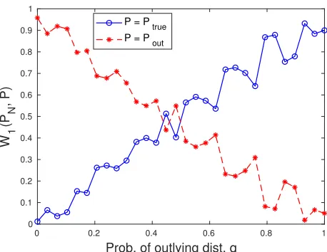
is further away. If the radius is chosen between the red (∗−) and blue (◦−) lines, the Wasserstein ball that we are hedging against will exclude the outlying distribution and the resulting estimator will be robust to the adversarial perturbations. Moreover, asqbecomes smaller, the gap between the red and blue lines becomes larger. One implication from this observation is that as the data becomes purer, the radius of the Wasserstein ball tends to be smaller, and the confidence in the observed samples is higher. For large q values, the DRO formulation seems to fail. However, as outliers are defined to be the data points that do not conform to the majority of data, we can safely claim thatPout is the distribution of

the minority andq is always below 0.5.

We now consider the inner supremum in (2). Esfahani and Kuhn (2015, Theorem 6.3) show that when the set Z is closed and convex, and the loss functionhβ(x, y) is convex in

(x, y),

sup

Q∈Ω

EQ[hβ(x, y)]≤κ+

1

N

X

i=1

(9)

0 0.2 0.4 0.6 0.8 1

Prob. of outlying dist. q

0 0.1 0.2 0.3 0.4 0.5 0.6 0.7 0.8 0.9 1

W

1

(P

N

, P)

P = P_true P = P_out

Figure 2: The order-1 Wasserstein distances from the empirical distribution.

whereκ(β) = sup{kθk∗ :h∗_β(θ)<∞}, withh∗_β(·) the convex conjugate function ofhβ(x, y).

Through (9), we can relax problem (2) by minimizing the right hand side of (9) instead of the worst-case expected loss. Moreover, as shown in Esfahani and Kuhn (2015), (9) becomes an equality when Z =Rm. In Theorem 2.1, we compute the value of κ(β) for the specific

`1 loss function we use. The proof of this Theorem and all results hereafter are included in

Appendix A.

Theorem 2.1 Defineκ(β) = sup{kθk∗ :h∗_β(θ)<∞}, wherek · k∗ is the dual norm ofk · k,

andh∗_β(·)is the conjugate function ofhβ(·). When the loss function is hβ(x, y) =|y−x0β|,

we have κ(β) =k(−β,1)k∗.

Due to Theorem 2.1, (2) could be formulated as the following optimization problem:

inf

β∈Bk(−β,1)k∗+

1

N

X

i=1

|yi−x0iβ|. (10)

Note that the regularization term of (10) is the product of thegrowth rateof the loss and the Wasserstein ball radius. The growth rate is closely related to the way the Wasserstein metric defines the transportation costs on the data (x, y). As mentioned earlier, a zero growth rate diminishes the effect of the Wasserstein distributional uncertainty set, and the resulting formulation would simply be an empirical loss minimization problem. The parameter

controls the conservativeness of the formulation, whose selection depends on the sample size, the dimensionality of the data, and the confidence that the Wasserstein ball contains the true distribution (see eq. (8) in Esfahani and Kuhn, 2015). Roughly speaking, when the sample size is large enough, and for a fixed confidence level,is inversely proportional toN1/m.

(10)

polyhedron with convex quadratic inequalities, (10) is a convex quadratic problem which can be solved to optimality very efficiently. Specifically, it could be converted to:

min

a, b1,...,bN,β

a+ 1

N

X

i=1

bi

s.t. kβk2₂+ 1≤a2,

yi−x0iβ≤bi, i= 1, . . . , N, −(yi−x0iβ)≤bi, i= 1, . . . , N,

a, bi≥0, i= 1, . . . , N,

β∈ B.

(11)

When the Wasserstein metric is defined usingk · k₁ and the set Bis a polyhedron, (10) is a linear programming problem:

min

a, b1,...,bN,β

a+ 1

N

X

i=1

bi

s.t. a≥β0ei, i= 1, . . . , m−1,

a≥ −β0ei, i= 1, . . . , m−1,

yi−x0iβ≤bi, i= 1, . . . , N, −(yi−x0iβ)≤bi, i= 1, . . . , N,

a≥1,

bi ≥0, i= 1, . . . , N,

β∈ B.

(12)

More generally, when the coordinates of (x, y) differ from each other substantially, a properly chosen, positive definite weight matrix M ∈ Rm×m could scale correspondingly different

coordinates of (x, y) by using theM-weighted norm:

k(x, y)k_M=p(x, y)0_M₍_x_{, y}₎_.

It can be shown that (10) in this case becomes:

inf

β∈B

p

(−β,1)0M−1₍₋_β_,_{1) +} 1 N

N

X

i=1

|yi−x0iβ|. (13)

(11)

brought by the Wasserstein DRO framework and justify the value and novelty of (10). First, (10) is obtained as an outcome of a fundamental DRO formulation, which enables new interpretations of the regularizer from the standpoint of distributional robustness, and provides rigorous theoretical foundation on why the `2-regularizer prevents overfitting to

the training data. The regularizer could be seen as a control over the amount of ambiguity in the data and reveals the reliability of the contaminated samples. Second, the geometry of the Wasserstein ball is embedded in the regularization term, which penalizes the regression coefficient on the dual Wasserstein space, with the magnitude of penalty being the radius of the ball. This offers an intuitive interpretation and provides guidance on how to set the regularization coefficient. Moreover, different from the traditional regularized LAD models that directly penalize the regression coefficient β, we regularize the vector (−β,1), where the 1 takes into account the transportation cost along the y direction. Penalizing only on

βcorresponds to an infinite transportation cost alongy. Our model is more general in this sense, and establishes the connection between the metric space on data and the form of the regularizer.

3. Performance Guarantees

Having obtained a tractable reformulation for the Wasserstein DRO problem, we next es-tablish guarantees on the predictive power and estimation quality for the solution to (10). Two types of results will be presented in this section, one of which bounds the prediction bias of the estimator on new, future data (given in Section 3.1). The other one that bounds the discrepancy between the estimated and true regression planes (estimation bias), is given in Section 3.2.

3.1 Out-of-Sample Performance

In this subsection we investigate generalization characteristics of the solution to (10), which involves measuring the error generated by our estimator on a new random sample (x, y). We would like to obtain estimates that not only explain the observed samples well, but, more importantly, possess strong generalization abilities. The derivation is mainly based on

Rademacher complexity(see Bartlett and Mendelson, 2002), which is a measurement of the

complexity of a class of functions. We would like to emphasize the applicability of such a proof technique to general loss functions, as long as their empirical Rademacher complexity could be bounded. The bound we derive for the prediction bias depends on both the sample average loss (the training error) and the dual norm of the regression coefficient (the regularizer), which corroborates the validity and necessity of our regularized formulation. Moreover, the generalization result also builds a connection between the loss function and the form of the regularizer via Rademacher complexity, which enables new insights into the regularization term and explains the commonly observed good out-of-sample performance of regularized regression in a rigorous way. We first make several mild assumptions that are needed for the generalization result.

Assumption A The norm of the uncertainty parameter (x, y) is bounded above almost

(12)

Assumption B The dual norm of (−β,1) is bounded above within the feasible region, namely,

sup

β∈B

k(−β,1)k∗ = ¯B.

Under these two assumptions, the absolute loss could be bounded via the Cauchy-Schwarz inequality.

Lemma 3.1 For every feasible β, it follows

|y−x0β| ≤BR,¯ almost surely.

With the above result, the idea is to bound the generalization error using the empirical

Rademacher complexityof the following class of loss functions:

H={(x, y)7→hβ(x, y) :hβ(x, y) =|y−x0β|, β∈ B}.

We need to show that the empirical Rademacher complexity of H, denoted by R_N(H), is upper bounded. The following result, similar to Lemma 3 in Bertsimas et al. (2015), provides a bound that is inversely proportional to the square root of the sample size.

Lemma 3.2

RN(H)≤

2 ¯BR

√

N .

Let ˆβ be an optimal solution to (10), obtained using the samples (xi, yi),i= 1, . . . , N.

Suppose we draw a new i.i.d. sample (x, y). In Theorem 3.3 we establish bounds on the error|y−x0βˆ|.

Theorem 3.3 Under Assumptions A and B, for any 0 < δ < 1, with probability at least

1−δ with respect to the sampling,

E[|y−x0βˆ|]≤ 1

N

X

i=1

|yi−x0iβˆ|+

2 ¯BR

√

N + ¯BR r

8 log(2/δ)

N , (14)

and for any ζ > 2 ¯√BR

N + ¯BR

q

8 log(2/δ)

N ,

P

|y−x0βˆ| ≥ 1

N

X

i=1

|yi−x0iβˆ|+ζ

≤

1

N

PN

i=1|yi−x

0

iβˆ|+2 ¯√BR_N + ¯BR

q

8 log(2/δ)

N

1

N

PN

i=1|yi−x0iβˆ|+ζ

. (15)

There are two probability measures in the statement of Theorem 3.3. One is related to the new data (x, y), while the other is related to the samples (x1, y1), . . . ,(xN, yN). The

(13)

are proportional to 1/√N. This result validates the dual norm-based regularized regression from the perspective of generalization ability, and could be generalized to any bounded loss function. It also provides implications on the form of the regularizer. For example, if given an `2-loss function, the dependency on ¯B for the generalization error bound will be of the

form ¯B2, which suggests using k(−β,1)k2

∗ as a regularizer, reducing to a variant of ridge

regression (Hoerl and Kennard, 1970) for k · k₂ induced Wasserstein metric.

We also note that the upper bounds in (14) and (15) do not depend on the dimension of (x, y). This dimensionality-free characteristic implies direct applicability of our Wasserstein approach to high-dimensional settings and is particularly useful in many real applications where, potentially, hundreds of features may be present. Theorem 3.3 also provides guidance on the number of samples that are needed to achieve satisfactory out-of-sample performance.

Corollary 3.4 Suppose βˆ is the optimal solution to (10). For a fixed confidence level δ

and some threshold parameter τ ≥ 0, to guarantee that the percentage difference between

the expected absolute loss on new data and the sample average loss is less than τ, that is,

E[|y−x0βˆ|]−_N1 PN_i₌₁|yi−x0iβˆ|

¯

BR ≤τ,

the sample size N must satisfy

N ≥

2(1 +p2 log(2/δ) )

τ

2

. (16)

Corollary 3.5 Suppose βˆ is the optimal solution to (10). For a fixed confidence level δ,

some τ ∈(0,1)and γ ≥0, to guarantee that

P

_|_y₋_x0_βˆ_{| −} 1

N

PN

i=1|yi−x

0

iβˆ|

¯

BR ≥γ

≤τ,

the sample size N must satisfy

N ≥

2(1 +p2 log(2/δ) )

τ·γ+τ −1

2

, (17)

provided that τ ·γ+τ −1>0.

In Corollaries 3.4 and 3.5, the sample size is inversely proportional to both δ and τ, which is reasonable since the more confident we want to be, the more samples we need. Moreover, the smaller τ is, the stricter a requirement we impose on the performance, and thus more samples are needed.

3.2 Discrepancy between Estimated and True Regression Planes

(14)

section we will use ˆβto denote the estimated regression coefficients, obtained as an optimal solution to (18), and β∗ for the true (unknown) regression coefficients. The bound we will derive turns out to be related to the Gaussian width (see definition in the Appendix) of the unit ball in k · k∞, the sub-Gaussian norm of the uncertainty parameter (x, y),

as well as the geometric structure of the true regression coefficients. We note that this proof technique may be applied to several other loss functions, e.g., `2 and `∞ losses, with

slight modifications. However, we will see that the `1-loss function incurs a relatively low

estimation bias compared to others, further demonstrating the superiority of our absolute error minimization formulation.

To facilitate the analysis, we will use the following equivalent form of problem (10):

min

β k(−β,1)k∗

s.t. k(−β,1)0Zk1 ≤γN,

β∈ B,

(18)

whereZ= [(x1, y1), . . . ,(xN, yN)] is the matrix with columns (xi, yi), i= 1, . . . , N, andγN

is some exogenous parameter related to. One can show that for properly chosenγN, (18)

produces the same solution with (10) (Bertsekas, 1999). (18) is similar to (11) in Chen and Banerjee (2016), with the difference lying in that we impose a constraint on the error instead of the gradient, and we consider a more general notion of norm on the coefficient. On the other hand, due to their similarity, we will follow the line of development in Chen and Banerjee (2016). Still, our analysis is self-contained and the bound we obtain is in a different form, which provides meaningful insights into our specific problem. We list below the assumptions that are needed to bound the estimation error.

Assumption C The`2norm of(−β,1)is bounded above within the feasible region, namely,

sup

β∈B

k(−β,1)k₂ = ¯B2.

Assumption D (Restricted Eigenvalue Condition) For some set A(β∗) =cone{v|

k(−β∗,1)+vk∗ ≤ k(−β∗,1)k∗}∩Sm and some positive scalarα, whereSm is the unit sphere

in the m-dimensional Euclidean space,

inf

v∈A(β∗)v

0_ZZ0_v_≥_α,

where Sm denotes the unit sphere in the m-dimensional Euclidean space.

Assumption E The true coefficient β∗ is a feasible solution to (18), i.e.,

kZ0(−β∗,1)k1≤γN, β∗∈ B.

Assumption F (x, y)is a centered sub-Gaussian random vector (see definition in the Ap-pendix), i.e., it has zero mean and satisfies the following condition:

|||(x, y)|||_ψ

2 = sup u∈_Sm

(x, y)0u

(15)

Assumption G The covariance matrix of (x, y) has bounded positive eigenvalues. Set

Γ=E[(x, y)(x, y)0]; then,

0< λmin,λmin(Γ)≤λmax(Γ),λmax<∞.

Notice that bothαin Assumption D andγN in Assumption E are related to the random

observation matrixZ. A probabilistic description for these two quantities will be provided later. We next present a preliminary result, similar to Lemma 2 in Chen and Banerjee (2016), that bounds the `2-norm of the estimation bias in terms of a quantity that is

related to the geometric structure of the true coefficients. This result gives a rough idea on the factors that affect the estimation error, and shows the advantages of using the `1-loss from the perspective of its dual norm. The bound derived in Theorem 3.6 is crude in the sense that it is a function of several random parameters that are related to the random observation matrix Z. This randomness will be described in a probabilistic way in the subsequent analysis.

Theorem 3.6 Suppose the true regression coefficient vector is β∗ and the solution to (18)

isβˆ. For the setA(β∗) =cone{v| k(−β∗,1)+vk∗ ≤ k(−β∗,1)k∗}∩Sm, under Assumptions

A, D, and E, we have:

kβˆ−β∗k2 ≤

2RγN

α Ψ(β

∗₎_, ₍₁₉₎

where Ψ(β∗) = sup_v∈A(β∗)kvk∗.

Notice that the bound in (19) does not explicitly depend on the sample size N. If we change to the`2-loss function, problem (18) will become:

min

β k(−β,1)k∗

s.t. k(−β,1)0Zk₂ ≤γN,

β∈ B.

The proof of Theorem 3.6 still applies with slight modification. We will find out that in the case of`2-loss, the estimation error bound takes the following form:

kβˆ −β∗k₂≤ 2R

√

N γN

α Ψ(β ∗₎_.

Similarly, the`∞-loss, which considers only the maximum absolute loss among the samples,

turns (18) into:

min

β k(−β,1)k∗

s.t. k(−β,1)0Zk∞≤γN,

β∈ B.

The corresponding bound becomes:

kβˆ−β∗k2 ≤

2RN γN

α Ψ(β ∗

(16)

We see that by using either`2 or`∞-loss, an explicit dependency on N is introduced. As a

result, the estimation error bounds become worse. The reason is that for the`1-loss function, its dual norm operator only picks out the maximum absolute coordinate and thus avoids the dependence on the dimension, which in our case is the sample size (see Eq.(28)), whereas other norms, e.g., `2-norm, sum over all the coordinates and thus introduce a dependence on N.

As mentioned earlier, (19) provides a random upper bound, revealed in α and γN, that

depends on the randomness inZ. We therefore would like to replace these two parameters by non-random quantities. Theαacts as the minimum eigenvalue of the matrixZZ0 restricted to a subspace of Rm, and thus a proper substitute should be related to the minimum

eigenvalue of the covariance matrix of (x, y), i.e., the Γ matrix (cf. Assumption G), given that (x, y) is zero mean. See Lemmas 3.7, 3.8 and 3.9 for the derivation.

Lemma 3.7 Consider the set A_Γ = {w ∈ _Sm_|_Γ−1/2_w _∈ _cone₍_A₍_β∗₎₎_{}, where} _A₍_β∗₎ _is

defined as in Theorem 3.6, and Γ = E[(x, y)(x, y)0]. Under Assumptions F and G, when

the sample size N ≥C1µ¯4(w(AΓ))2, where µ¯ =µ

q 1

λmin, andw(AΓ) is the Gaussian width

of A_Γ, with probability at least 1−exp(−C2N/µ¯4), we have

v0ZZ0v≥ N

2v

0_Γv_, _∀ _v_{∈ A}₍_β∗₎_,

where C1 and C2 are positive constants.

Note that the sample size requirement stated in Lemma 3.7 depends on the Gaussian width of AΓ, whereAΓ relates to A(β∗). The following lemma shows that their Gaussian widths

are also related. This relation is built upon the square root of the eigenvalues of Γ, which measures the extent to whichA_Γ expands A(β∗).

Lemma 3.8 (Lemma 4 in Chen and Banerjee (2016)) Let µ0 be the ψ2-norm of a

standard Gaussian random vector g ∈ Rm, and AΓ, A(β∗) be defined as in Lemma 3.7.

Then, under Assumption G,

w(A_Γ)≤C3µ0 r

λmax

λmin

w(A(β∗)) + 3,

for some positive constant C3.

Combining Lemmas 3.7 and 3.8, and expressing the covariance matrixΓusing its eigenval-ues, we arrive at the following result.

Corollary 3.9 Under Assumptions F and G, and the conditions in Lemmas 3.7 and 3.8,

when N ≥C1¯µ¯4µ2₀·λmax

λmin

w(A(β∗)) + 3

2

, with probability at least 1−exp(−C2N/µ¯4),

v0ZZ0v≥ N λmin

2 , ∀ v∈ A(β

∗

),

(17)

Next, we derive the smallest possible value ofγN such thatβ∗ is feasible. The derivation

uses the dual norm operator of the`1-loss, resulting in a bound that depends on the Gaussian width of the unit ball in the dual norm space (k · k∞). See Lemma 3.10 for details.

Lemma 3.10 Under Assumptions C and F, for any feasible β, with probability at least

1−C4exp(−C

2

5(w(Bu))2

4ρ2 ),

k(−β,1)0Zk1 ≤CµB2¯ w(Bu),

whereBu is the unit ball of normk · k∞,ρ= supv∈Bukvk2, andC4, C5, C positive constants.

We note that for other loss functions, e.g., the `2 and `∞ losses, similar results can be

obtained, where Bu is defined to be the unit k · kloss∗ -ball in Rm, with k · kloss∗ being the

dual norm of the loss. Combining Theorem 3.6, Corollary 3.9 and Lemma 3.10, we have the following main performance guarantee result that bounds the estimation bias of the solution to (18).

Theorem 3.11 Under Assumptions A, C, D, E, F, G, and the conditions of Theorem 3.6,

Corollary 3.9 and Lemma 3.10, when N ≥C¯1µ¯4µ20·λλmaxmin

w(A(β∗)) + 32, with probability

at least 1−exp(−C2N/µ¯4)−C4exp(−C₅2(w(Bu))2/(4ρ2)),

kβˆ−β∗k2 ≤

¯

CRB2µ¯ N λmin

w(Bu)Ψ(β∗). (20)

From (20) we see that the bias is decreased as the sample size increases and the uncer-tainty embedded in (x, y) (revealed in R and µ) is reduced. The estimation error bound depends on the geometric structure of the true coefficients, defined using the dual norm space of the Wasserstein metric, the Gaussian width of the unit k · kloss

∗ -ball in Rm, and

the minimum eigenvalue of the covariance matrix of (x, y), with a convergence rate 1/N for the `1-loss we applied. As mentioned earlier, other loss functions may incur a dependence

on N in the numerator of the bound, thus resulting in a slower convergence rate, which substantiates the benefit of using an`1-loss function.

4. Simulation Experiments on Synthetic Datasets

In this section we will explore the robustness of the Wasserstein formulation in terms of

its Absolute Deviation (AD) loss function and the dual norm regularizer on the extended

regression coefficient (−β,1). Recall that our Wasserstein formulation is in the following

form:

inf

β∈B

1

N

X

i=1

|yi−x0iβ|+k(−β,1)k∗. (21)

We will focus on the following three aspects of this formulation:

1. How to choose a proper norm k · kfor the Wasserstein metric?

2. Why do we penalize the extended regression coefficient (−β,1) rather thanβ?

(18)

To answer Question 1, we will connect the choice of k · k for the Wasserstein metric with the characteristics/structures of the data (x, y). Specifically, we will design two sets of experiments, one with a dense regression coefficientβ∗, where all coordinates ofxplay a role in determining the value of the responsey, and another with a sparseβ∗ implying that only a few predictors are relevant/important in predictingy. Two Wasserstein formulations will be tested and compared, one induced by thek · k₂ (Wasserstein `2), which leads to an `2-regularizer in (21), and the other one induced by thek·k∞(Wasserstein`∞) and resulting

in an`1-regularizer in (21). Intuitively, and based on the past experience in implementing the regularization techniques, the Wasserstein `2 should outperform the Wasserstein `∞

in the dense setting, while in the sparse setting, the reverse is true. Researchers have well identified the sparsity inducing property of the`1-regularizer and provided a nice geometrical interpretation for it (Friedman et al., 2001). Here, we try to offer a different explanation from the perspective of the Wasserstein DRO formulation, through projecting the sparsity of β∗ onto the (x, y) space and establishing a sparse distance metric that only extracts a subset of coordinates from (x, y) to measure the closeness between samples.

For the second question, we first note that if the Wasserstein metric is induced by the following metricsc:

sc(x, y) =k(x, cy)k2,

for a positive constant c, then as c → ∞, the resulting Wasserstein DRO formulation becomes:

inf

β∈B

1

N

X

i=1

|yi−x0iβ|+kβk2,

which is the `2-regularized LAD. This can be proved by recognizing that sc(x, y) = k(x, y)kM, with M∈ Rm×m a diagonal matrix whose diagonal elements are (1, . . . ,1, c2),

and then applying (13). Alternatively, if we let

sc(x, y) =k(x, cy)k∞,

it can be shown that as c→ ∞, the corresponding Wasserstein formulation becomes:

inf

β∈B

1

N

X

i=1

|yi−x0iβ|+kβk1,

which is the `1-regularized LAD (see proof in the Appendix). It follows that regularizing

overβ implies an infinite transportation cost along y. In other words, for two data points (x1, y1) and (x2, y2), if y1 6= y2, then they are considered to be infinitely far away. By

contrast, our Wasserstein formulation, which regularizes over the extended regression coef-ficient (−β,1), stems from a finite cost alongy that is equally weighted withx. We will see the disadvantages of penalizing onlyβ in the analysis of the experimental results.

(19)

by the residuals. These models will be compared under two different experimental setups, one involving adversarial perturbations in both x and y, and the other with perturbations only in x. The purpose is to investigate the behavior of these approaches when the noise in y is substantially reduced. As shown by Fig. 1, compared to the SR loss, the AD loss is less vulnerable to large residuals, and hence, it is advantageous in the scenarios where large perturbations appear in y. We are interested in studying whether its performance is consistently good when the corruptions appear mainly inx.

We next describe the data generation process. Each training sample has a probability

q of being drawn from the outlying distribution, and a probability 1−q of being drawn from the true (clean) distribution. Given the true regression coefficientβ∗, we generate the training data as follows:

• Generate a uniform random variable on [0,1]. If it is no larger than 1−q, generate a clean sample as follows:

1. Draw the predictorx ∈Rm−1 from the normal distribution Nm−1(0,Σ), where Σis the covariance matrix of x, which is just the top left block of the matrixΓ

in Assumption G. Specifically,Γ=E[(x, y)(x, y)0] is equal to

Γ=

Σ Σβ∗

(β∗)0Σ (β∗)0Σβ∗+σ2

,

with σ2 being the variance of the noise term. In our implementation, Σ has diagonal elements equal to 1 (unit variance) and off-diagonal elements equal to

ρ, with ρ the correlation between predictors.

2. Draw the response variable y fromN(x0β∗, σ2).

• Otherwise, depending on the experimental setup, generate an outlier that is either:

– Abnormal in both xand y, with outlying distribution:

1. x∼Nm−1(0,Σ) +Nm−1(5e,I), orx∼Nm−1(0,Σ) +Nm−1(0,0.25I);

2. y∼N(x0β∗, σ2) + 5σ.

– Abnormal only in x:

1. x∼Nm−1(0,Σ) +Nm−1(5e,I);

2. y∼N(x0β∗, σ2).

• Repeat the above procedure for N times, where N is the size of the training set.

(20)

• Signal to Noise Ratio (SNR), defined as:

SNR = (β

∗

)0Σβ∗

σ2 ,

which is equally spaced between 0.05 and 2 on a log scale.

• The correlation between predictors: ρ, which takes values in (0.1,0.2, . . . ,0.9).

The performance metrics we use include:

• Mean Squared Error (MSE) on the test dataset, which is defined to be PM

i=1(yi−

x0_iβˆ)2/M, with ˆβ being the estimate of β∗ obtained from the training set, and (xi, yi), i= 1, . . . , M,being the observations from the test dataset;

• Relative Risk (RR) of ˆβ defined as:

RR( ˆβ), ( ˆβ−β

∗

)0Σ( ˆβ−β∗) (β∗)0_Σ_β∗ .

• Relative Test Error (RTE)of ˆβdefined as:

RTE( ˆβ), ( ˆβ−β

∗₎0_Σ_{( ˆ}_β₋_β∗_{) +}_σ2

σ2 .

• Proportion of Variance Explained (PVE)of ˆβ defined as:

PVE( ˆβ),1− ( ˆβ−β

∗

)0Σ( ˆβ−β∗) +σ2

(β∗)0_Σ_β∗₊_σ2 .

For the metrics that evaluate the accuracy of the estimator, i.e., the RR, RTE and PVE, we list below two types of scores, one achieved by the best possible estimator ˆβ =β∗, called the perfect score, and the other one achieved by the null estimator ˆβ = 0, called the null score.

• RR: a perfect score is 0 and the null score is 1.

• RTE: a perfect score is 1 and the null score is SNR+1.

• PVE: a perfect score is _SNR+1SNR , and the null score is 0.

During the training process, all the regularization parameters are tuned on a separate validation dataset. Specifically, we divide all theN training samples into two sets, dataset 1 and dataset 2 (validation set). For a pre-specified range of values for the penalty parameters, dataset 1 is used to train the models and derive ˆβ, and the performance of ˆβ is evaluated on dataset 2. We choose the regularization parameter that yields the minimum Median

Absolute Deviation (MAD)on the validation set. Using MAD as a selection criterion serves

(21)

LASSO was tuned over 50 values ranging fromλm =kX0yk∞to a small fraction ofλm on a

log scale, with X∈RN×(m−1) the design matrix whosei-th row isx0i, and y= (y1, . . . , yN)

the response vector. In our experiments, this range is properly adjusted for procedures that use the AD loss. Specifically, for Wasserstein `2 and `∞, `1- and `2-regularized LAD, the

range of values for the regularization parameter is:

s

exp

linlog(0.005∗ kX0_y_k

∞),log(kX0yk∞),50

,

where lin(a, b, n) is a function that takes in scalars a, b and n (integer) and outputs a set of n values equally spaced between a and b; the exp function is applied elementwise to a vector. The square root operator is in consideration of the AD loss that is the square root of the SR loss if evaluated on a single sample.

The regularization coefficientin formulation (10), which is the radius of the Wasserstein ball, allows for a more efficient tuning procedure. It has been noted in Esfahani and Kuhn (2015) that for a large enough sample size, is inversely proportional to N1/m_. _This

proportionality could be used as a guidance on setting, where only the proportional factor needs to be tuned (using cross-validation or a separate validation dataset as described earlier). In our implementation, given the small size of the simulated datasets, we will still adopt the validation dataset approach to tune the regularization parameter.

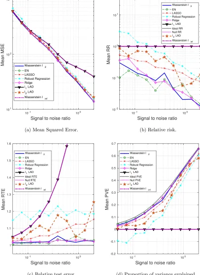
4.1 Dense β∗, outliers in both x and y

In this subsection, we choose a dense regression coefficient β∗, set the intercept β₀∗ = 0.3, and the coefficient for each predictor xi to be β∗_i = 0.5, i = 1, . . . ,20. The adversarial

perturbations are present in bothxandy. Specifically, the outlying distribution is described by:

1. x∼Nm−1(0,Σ) +Nm−1(5e,I);

2. y∼N(x0β∗, σ2) + 5σ.

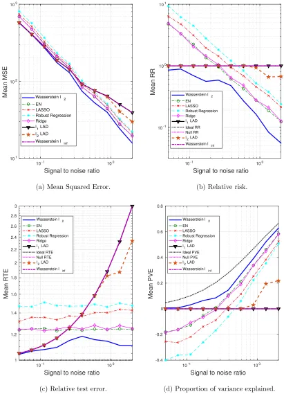
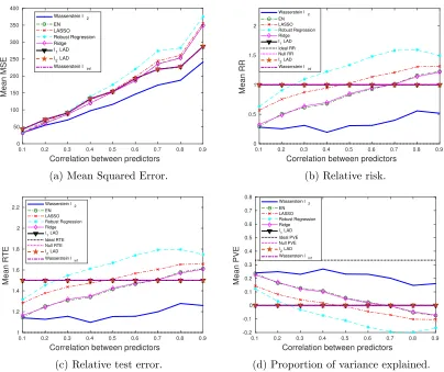
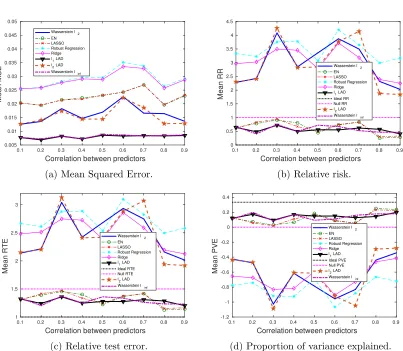
We generate 10 datasets consisting of N = 100, M = 60 observations. The probability of a training sample being drawn from the outlying distribution is q = 30%. The mean values of the performance metrics (averaged over the 10 datasets), as we vary the SNR and the correlation between predictors, are shown in Figs. 3 and 4. Note that when SNR is varied, the correlation between predictors is set to 0.8 times a random noise uniformly distributed on the interval [0.2,0.4]. When the correlationρ is varied, the SNR is fixed to 0.5.

It can be seen that as the SNR decreases or the correlation between the predictors increases, the estimation problem becomes harder, and the performance of all approaches gets worse. In general the Wasserstein`2 achieves the best performance in terms of all four

metrics. Specifically,

• It is better than the `2-regularized LAD, which assumes an infinite transportation

cost alongy.

• It is better than the Wasserstein `∞ and `1-regularized LAD which use the `1

(22)

• It is better than the approaches that use the SR loss function.

Empirically we have found out that in most cases, the approaches that use the AD loss, including the`1- and `2-regularized LAD, and the Wasserstein`∞formulation, drive all the

coordinates ofβto zero, due to the relatively small magnitude of the AD loss compared to the norm of the coefficient, so that the regularizer dominates the solution. The approaches that use the SR loss, e.g., ridge regression and EN, do not exhibit such a problem, since the squared residuals weaken the dominance of the regularization term.

Overall the `2-regularizer outperforms the `1-regularizer, since the true regression co-efficient is dense, which implies that a proper distance metric on the (x, y) space should take into account all the coordinates. From the perspective of the Wasserstein DRO frame-work, the `1-regularizer corresponds to an k · k∞-based distance metric on the (x, y) space

that only picks out the most influential coordinate to determine the closeness between data points, which in our case is not reasonable since every coordinate plays a role (reflected in the dense β∗). In contrast, ifβ∗ is sparse, using thek · k∞ as a distance metric on (x, y) is

more appropriate. A more detailed discussion of this will be presented in Sections 4.3 and 4.4.

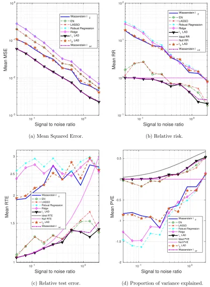
4.2 Dense β∗, outliers only in x

In this subsection we will experiment with the same β∗ as in Section 4.1, but with per-turbations only in x, i.e., for a given x of the outlier, the corresponding y value is drawn in the same way as the clean samples. Our goal is to investigate the performance of the Wasserstein formulation when the response y is not subjected to large perturbations. The motivation for introducing the AD loss in the Wasserstein formulation is to hedge against large residuals, as illustrated in Fig. 1. We are interested in comparing the AD and SR loss functions when the residuals have moderate magnitudes.

Interestingly, we have observed that although the `1- and `2-regularized LAD, as well as the Wasserstein`∞formulation, exhibit unsatisfactory performance, the Wasserstein `2,

which shares the same loss function with them, is able to achieve a comparable performance with the best among all – EN and ridge regression (see Figs. 5 and 6). Notably, the `2 -regularized LAD, which is just slightly different from our Wasserstein`2formulation, shows

a much worse performance. This is because the `2-regularized LAD implicitly assumes

an infinite transportation cost along y, which gives zero tolerance to the variation in the response. For example, given two data points (x1, y1) and (x2, y2), as long as y1 6=y2, the distance between them is infinity. Therefore, a reasonable amount of fluctuation, caused by the intrinsic randomness ofy, would be overly exaggerated by the underlying metric used by the`2-regularized LAD. In contrast, our Wasserstein approach uses a proper notion of norm to evaluate the distance in the (x, y) space and is able to effectively distinguish abnormally high variations from moderate, acceptable noise.

It is also worth noting that the formulations with the AD loss, e.g.,`2- and`1-regularized LAD, and the Wasserstein `∞, perform worse than the approaches with the SR loss. One

(23)

10-1 100

Signal to noise ratio

101 102 103

Mean MSE Wasserstein l ₂

EN LASSO Robust Regression Ridge

l₁ LAD

l₂ LAD Wasserstein l _inf

(a) Mean Squared Error.

10-1 100

Signal to noise ratio 10-1

100 101

Mean RR Wasserstein l ₂ EN LASSO Robust Regression Ridge l1 LAD Ideal RR Null RR l₂ LAD Wasserstein l inf

(b) Relative risk.

10-1 ₁₀0

1 1.2 1.4 1.6 1.8 2 2.2 2.4 2.6 2.8 3

Mean RTE

Wasserstein l ₂

EN LASSO Robust Regression Ridge l1 LAD

Ideal RTE Null RTE l₂ LAD

Wasserstein l inf

(c) Relative test error.

10-1 ₁₀0

-0.4 -0.2 0 0.2 0.4 0.6 0.8

Mean PVE

Wasserstein l ₂ EN LASSO Robust Regression Ridge l1 LAD Ideal PVE Null PVE l₂ LAD

Wasserstein l inf

(d) Proportion of variance explained.

Figure 3: The impact of SNR on the performance metrics: denseβ∗, outliers in bothxand

(24)

0.1 0.2 0.3 0.4 0.5 0.6 0.7 0.8 0.9

Correlation between predictors

0 50 100 150 200 250 300 350 400

Mean MSE

Wasserstein l2 EN LASSO Robust Regression Ridge l1 LAD l₂ LAD Wasserstein linf

0.1 0.2 0.3 0.4 0.5 0.6 0.7 0.8 0.9

0 0.5 1 1.5 2

Mean RR

Wasserstein l2 EN LASSO Robust Regression Ridge l₁ LAD Ideal RR Null RR l2 LAD Wasserstein l_inf

(b) Relative risk.

0.1 0.2 0.3 0.4 0.5 0.6 0.7 0.8 0.9 Correlation between predictors

1 1.2 1.4 1.6 1.8 2 2.2

Mean RTE

Wasserstein l2 EN LASSO Robust Regression Ridge l₁ LAD Ideal RTE Null RTE l2 LAD Wasserstein l_inf

0.1 0.2 0.3 0.4 0.5 0.6 0.7 0.8 0.9

-0.2 -0.1 0 0.1 0.2 0.3 0.4 0.5 0.6 0.7 0.8

Mean PVE

Wasserstein l₂

l₁ LAD

Ideal PVE Null PVE

l₂ LAD

Wasserstein linf

(25)

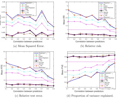
the extended coefficient vector (−β,1) seems to make up, making the Wasserstein `2 a

competitive method even when the perturbations appear only inx.

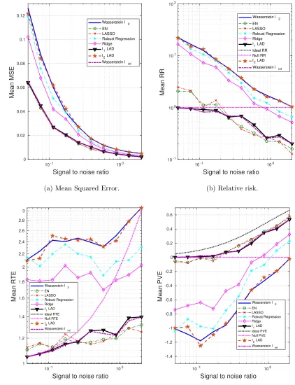
4.3 Sparse β∗, outliers in both x and y

In this subsection we will experiment with a sparse β∗. The intercept is set to β₀∗= 3, and the coefficients for the 20 predictors are set toβ∗= (0.05,0,0.006,0,−0.007,0,0.008,0, . . . ,0). The adversarial perturbations are present in both x and y. Specifically, the distri-bution of outliers is characterized by:

1. x∼Nm−1(0,Σ) +Nm−1(0,0.25I);

2. y∼N(x0β∗, σ2) + 5σ.

Our goal is to study the impact of the sparsity of β∗ on the choice of the norm space for the Wasserstein metric. We know that the `1-regularizer works better than the `2

-regularizer for sparse data, which has been validated by our results in Figs. 7 and 8. We will see that the Wasserstein `∞ formulation significantly outperforms the Wasserstein `2. An intuitively appealing interpretation for the sparsity inducing property of the `1

-regularizer is made available by the Wasserstein DRO framework, which we explain as follows. The sparse regression coefficient β∗ implies that only a few predictors are relevant to the regression model, and thus when measuring the distance in the (x, y) space, we need a metric that only extracts the subset of relevant predictors. Thek · k∞, which takes only

the most influential coordinate of its argument, roughly serves this purpose. Compared to

thek · k2 which takes into account all the coordinates, most of which are redundant due to

the sparsity assumption,k · k∞ results in a better performance, and hence, the Wasserstein `∞ formulation that stems from the k · k∞ distance metric on (x, y) and induces the `1

-regularizer is expected to outperform others.

We note that the `1-regularized LAD achieves similar performance to ours, since

re-placing kβk1 by k(−β,1)k1 only adds a constant term to the objective function. The

generalization performance (mean MSE) of the AD loss-based formulations is consistently better than those with the SR loss, since the AD loss is less affected by large perturbations iny. Also note that choosing a wrong norm for the Wasserstein metric, e.g., the Wasserstein

`2, could lead to an enormous estimation error, whereas with a right norm space, we are guaranteed to outperform all others. Even when the SNR is very low, our performance is at least as good as the null estimator (see Fig. 7). Although EN and LASSO achieve similar performance to ours for moderate SNR values, they have a chance of performing even worse than the null estimator when there is little signal/information to learn from.

4.4 Sparse β∗, outliers only in x

In this subsection, we will use the same sparse coefficient as in Section 4.3, but the pertur-bations are present only in x. Specifically, for outliers, their predictors and responses are drawn from the following distributions:

1. x∼Nm−1(0,Σ) +Nm−1(5e,I);

(26)

10-1 100

101 102 103

Mean MSE Wasserstein l ₂

l₁ LAD l₂ LAD

Wasserstein l _inf

10-1 100

10-1 100 101

Mean RR

Wasserstein l ₂ EN LASSO Robust Regression Ridge l₁ LAD Ideal RR Null RR l₂ LAD Wasserstein l _inf

(b) Relative risk.

10-1 100

1 1.1 1.2 1.3 1.4 1.5 1.6

Mean RTE

Wasserstein l ₂ EN LASSO Robust Regression Ridge l₁ LAD Ideal RTE Null RTE l2 LAD Wasserstein l _inf

10-1 100

-0.2 -0.1 0 0.1 0.2 0.3 0.4 0.5 0.6 0.7

Mean PVE

Wasserstein l ₂

l₁ LAD

Ideal PVE Null PVE

l2 LAD

Wasserstein l _inf

(27)

0.1 0.2 0.3 0.4 0.5 0.6 0.7 0.8 0.9

0 50 100 150 200 250 300

Mean MSE

Wasserstein l2 EN LASSO Robust Regression Ridge l1 LAD l₂ LAD Wasserstein linf

0.1 0.2 0.3 0.4 0.5 0.6 0.7 0.8 0.9

0 0.2 0.4 0.6 0.8 1

Mean RR

(b) Relative risk.

0.9 1 1.1 1.2 1.3 1.4 1.5

Mean RTE

Wasserstein l2 EN LASSO Robust Regression Ridge l1 LAD Ideal RTE Null RTE l2 LAD Wasserstein l_inf

0.1 0.2 0.3 0.4 0.5 0.6 0.7 0.8 0.9

0 0.05 0.1 0.15 0.2 0.25 0.3 0.35 0.4

Mean PVE

Wasserstein l₂ EN LASSO Robust Regression Ridge l₁ LAD Ideal PVE Null PVE l₂ LAD Wasserstein linf

(28)

10-1 100

10-3 10-2 10-1 100

Mean MSE

Wasserstein l ₂

EN LASSO Robust Regression Ridge l1 LAD

l₂ LAD

Wasserstein l _inf

10-1 100

100 101 102

Mean RR

Wasserstein l 2 EN LASSO Robust Regression Ridge l₁ LAD Ideal RR Null RR l2 LAD Wasserstein l _inf

(b) Relative risk.

10-1 ₁₀0

Signal to noise ratio 1

1.5 2 2.5 3

Mean RTE

Wasserstein l₂

l₁ LAD

Ideal RTE Null RTE l

2 LAD

Wasserstein l_inf

10-1 ₁₀0

Signal to noise ratio -2

-1.5 -1 -0.5 0 0.5

Mean PVE _{Wasserstein l}

2

l₁ LAD

Ideal PVE Null PVE l

2 LAD

Wasserstein l_inf

Figure 7: The impact of SNR on the performance metrics: sparse β∗, outliers in both x

(29)

0.1 0.2 0.3 0.4 0.5 0.6 0.7 0.8 0.9

0.005 0.01 0.015 0.02 0.025 0.03 0.035 0.04 0.045 0.05

Mean MSE

Wasserstein l2

EN LASSO Robust Regression Ridge l₁ LAD l2 LAD

Wasserstein linf

0.1 0.2 0.3 0.4 0.5 0.6 0.7 0.8 0.9

0 0.5 1 1.5 2 2.5 3 3.5 4 4.5

Mean RR

(b) Relative risk.

1 1.5 2 2.5 3

Mean RTE

Wasserstein l₂ EN LASSO Robust Regression Ridge l1 LAD Ideal RTE Null RTE l2 LAD Wasserstein l_inf

0.1 0.2 0.3 0.4 0.5 0.6 0.7 0.8 0.9

-1.2 -1 -0.8 -0.6 -0.4 -0.2 0 0.2 0.4

Mean PVE

Wasserstein l₂

l1 LAD

Ideal PVE Null PVE

l₂ LAD

Wasserstein l_inf

(30)

Not surprisingly, the Wasserstein `∞ and the `1-regularized LAD achieve the best

per-formance. Notice that in Section 4.3, where perturbations appear in bothxand y, the AD based formulations have smaller generalization and estimation errors than the SR loss-based formulations. When we reduce the variation in y, the SR loss seems superior to the AD loss, if we restrict attention to the improperly regularized (`2-regularizer) formulations (see Fig. 9). For the `1-regularized formulations, our Wasserstein `∞ formulation, as well

as the `1-regularized LAD, is comparable with the EN and LASSO. Moreover, when there

is little information to utilize (low SNR), EN and LASSO are worse than the null estimator, whereas our performance is at least as good as the null estimator.

We summarize below our main findings from all sets of experiments we have presented:

1. When a proper norm space is selected for the Wasserstein metric, the Wasserstein DRO formulation outperforms all others in terms of the generalization and estimation qualities.

2. Penalizing the extended regression coefficient (−β,1) implicitly assumes a more rea-sonable distance metric on (x, y) and thus leads to a better performance.

3. The AD loss is remarkably superior to the SR loss when there is large variation in the responsey.

4. The Wasserstein DRO formulation shows a more stable estimation performance than others when the correlation between predictors is varied.

4.5 An outlier detection example

As an application, we consider an unlabeled two-class classification problem, where our goal is to identify the abnormal class of data points based on the predictor and response information using the Wasserstein formulation. We do not know a priori whether the samples are normal or abnormal, and thus classification models do not apply. The commonly used regression model for this type of problem is the M-estimation (Huber, 1964, 1973), against which we will compare in terms of the outlier detection capability.

The data are generated in the same fashion as before. For clean samples, all predictors

x1, . . . , x30come from a normal distribution with mean 7.5 and standard deviation 4.0. The

response is a linear function of the predictors with β∗₀ = 0.3, β₁∗ = · · · = β₃₀∗ = 0.5, plus a Gaussian distributed noise term with zero mean and standard deviationσ. The outliers concentrate in a cloud that is randomly placed in the interior of the x-space. Specifically, their predictors are uniformly distributed on (u−0.125, u+ 0.125), where u is a uniform random variable on (7.5−3×4,7.5 + 3×4). The response values of the outliers are at a

δR distance off the regression plane.

y=β∗₀+β₁∗x1+· · ·+β∗₃₀x30+δR.

We will compare the performance of the Wasserstein `2 formulation (10) with the `1

(31)

10-1 100

0 0.02 0.04 0.06 0.08 0.1 0.12

Mean MSE

Wasserstein l 2

EN LASSO Robust Regression Ridge l₁ LAD

l₂ LAD

Wasserstein l _inf

10-1 100