Stochastic Variance-Reduced Cubic Regularization Methods

(1)

Stochastic Variance-Reduced Cubic Regularization Methods

Department of Computer Science University of California, Los Angeles Los Angeles, CA 90095, USA

Editor:Zhihua Zhang

Abstract

We propose a stochastic variance-reduced cubic regularized Newton method (SVRC) for non-convex optimization. At the core of SVRC is a novel semi-stochastic gradient along with a semi-stochastic Hessian, which are specifically designed for cubic regularization method. For a nonconvex function withncomponent functions, we show that our algorithm is guaranteed to converge to an (,√)-approximate local minimum within Oe(n4/5/3/2)1

second-order oracle calls, which outperforms the state-of-the-art cubic regularization algo-rithms including subsampled cubic regularization. To further reduce the sample complexity of Hessian matrix computation in cubic regularization based methods, we also propose a sample efficient stochastic variance-reduced cubic regularization (Lite-SVRC) algorithm for finding the local minimum more efficiently. Lite-SVRC converges to an (,√)-approximate local minimum within Oe(n+n2/3/3/2) Hessian sample complexity, which is faster than

all existing cubic regularization based methods. Numerical experiments with different non-convex optimization problems conducted on real datasets validate our theoretical results for both SVRC and Lite-SVRC.

Keywords: Cubic Regularization, Nonconvex Optimization, Variance Reduction, Hessian Sample Complexity, Local Minimum

1. Introduction

We study the following unconstrained finite-sum nonconvex optimization problem:

min

x∈Rd

F(x) := 1 n

n

X

i=1

fi(x), (1)

1. HereOehides poly-logarithmic factors.

c

(2)

where each fi : Rd → R is a general nonconvex function. Such nonconvex optimization

problems are ubiquitous in machine learning, including training deep neural network (LeCun et al., 2015), robust linear regression (Yu and Yao, 2017) and nonconvex regularized logistic regression (Reddi et al., 2016b). In principle, finding the global minimum of (1) is generally a NP-hard problem (Hillar and Lim, 2013) due to the lack of convexity.

Instead of finding the global minimum, various algorithms have been developed in the lit-erature (Nesterov and Polyak, 2006; Cartis et al., 2011a; Carmon and Duchi, 2016; Agarwal et al., 2017; Xu et al., 2018b; Allen-Zhu and Li, 2018) to find an approximate local minimum of (1). In particular, a point xis said to be an (g, H)-approximate local minimum ofF if

k∇F(x)k₂ ≤g, λmin(∇2F(x))≥ −H, (2)

whereg, H >0 are predefined precision parameters. It has been shown that such

approx-imate local minima can be as good as global minima in some problems. For instance, Ge et al. (2016) proved that any local minimum is actually a global minimum in matrix comple-tion problems. Therefore, to develop an algorithm to find an approximate local minimum is of great interest both in theory and practice.

A very important and popular method to find the approximate local minimum is cubic-regularized (CR) Newton method, which was originally introduced by Nesterov and Polyak (2006). Generally speaking, in thek-th iteration, CR solves a sub-problem which minimizes a cubic-regularized second-order Taylor expansion at current iterate xk. The update rule

can be written as follows:

hk= argmin h∈_Rd

h∇F(xk),hi+

1 2h∇

2_F₍_x

k)h,hi+

M 6 khk

3

2, (3)

xk+1 =xk+hk, (4)

whereM >0 is a penalty parameter used in CR. Nesterov and Polyak (2006) proved that to find an (,√)-approximate local minimum of a nonconvex function F, CR requires at most O(−3/2_{) iterations. However, a major drawback for CR is that it needs to sample} n individual gradients ∇fi(xk) and Hessian matrices ∇2fi(xk) in (3) at each iteration,

which leads to a totalO(n−3/2) Hessian sample complexity, i.e., number of queries to the stochastic Hessian ∇2_f

i(x) for some i and x. Such computational cost will be extremely

expensive whenn is large as in many large scale machine learning problems.

To overcome the computational burden of CR based methods, some recent studies have proposed to use sub-sampled Hessian instead of the full Hessian (Kohler and Lucchi, 2017; Xu et al., 2017a) to reduce the Hessian complexity. In detail, Kohler and Lucchi (2017) proposed a sub-sampled cubic-regularized Newton method (SCR), which uses a subsampled Hessian instead of full Hessian to reduce the per iteration sample complexity of Hessian evaluations. Xu et al. (2017a) proposed a refined convergence analysis of SCR, as well as a subsampled Trust Region algorithm (Conn et al., 2000). Nevertheless, SCR bears a much slower convergence rate than the original CR method, and the total Hessian sample complexity for SCR to achieve an (,√)-approximate local minimum is O(e −5/2). This suggests that the computational cost of SCR could be even worse than CR when.n−1.

(3)

2016; Reddi et al., 2016a) into the cubic-regularized Newton method. The key component in our algorithm is a novel semi-stochastic gradient, together with a semi-stochastic Hes-sian, that are specifically designed for cubic regularization. Furthermore, we prove that, forL2-Hessian Lipschitz functions, to attain an (,

√

L2)-approximate local minimum, our proposed algorithm requiresO(n+n4/5/3/2) Second-order Oracle (SO) calls andO(1/3/2) Cubic Subproblem Oracle (CSO) calls. Here an SO oracle represents an evaluation of triple (fi(x),∇fi(x),∇2fi(x)), and a CSO oracle denotes an evaluation of the exact solution (or

inexact solution) of the cubic subproblem (3). Compared with the original cubic regu-larization algorithm (Nesterov and Polyak, 2006), which requires O(n/3/2) SO calls and O(1/3/2) CSO calls, our proposed SVRC algorithm reduces the SO calls by a factor of Ω(n1/5).

The second-order oracle complexity is dominated by the maximum number of queries to one of the elements in the triplet (fi(x),∇fi(x),∇2fi(x)), and therefore is not always

desirable in reflecting the computational complexity of multifarious applications. Therefore, we need to focus more on the Hessian sample complexity of cubic regularization methods for relatively high dimensional problems. Based on the SVRC algorithm, in order to further reduce the Hessian sample complexity, we also develop a sample efficient stochastic variance-reduced cubic-regularized Newton method called Lite-SVRC, which significantly reduces the sample complexity of Hessian matrix evaluations in stochastic CR methods. Under mild conditions, we prove that Lite-SVRC achieves a lower Hessian sample complexity than existing cubic regularization based methods. We prove that Lite-SVRC converges to an (,√)-approximate local minimum of a nonconvex function within O(ne +n2/3−3/2) Hessian sample complexity.

We summarize the major contributions of this paper as follows:

• We present a novel cubic regularization method (SVRC) with improved oracle com-plexity. To the best of our knowledge, this is the first algorithm that outperforms cubic regularization without any loss in convergence rate. In sharp contrast, existing subsampled cubic regularization methods (Kohler and Lucchi, 2017; Xu et al., 2017a) suffer from worse convergence rates than cubic regularization.

• We also extend SVRC to the case with inexact solution to the cubic regularization subproblem. Similar to previous work (Cartis et al., 2011a; Xu et al., 2017a), we layout a set of sufficient conditions, under which the output of the inexact algorithm is still guaranteed to have the same convergence rate and oracle complexity as the exact algorithm. This further sheds light on the practical implementation of our algorithm.

• As far as we know, our work is the first to rigorously demonstrate the advantage of variance reduction for second-order optimization algorithms. Although there exist a few studies (Lucchi et al., 2015; Moritz et al., 2016; Rodomanov and Kropotov, 2016) using variance reduction to accelerate Newton method, none of them can deliver faster rates of convergence than standard Newton method.

(4)

• We conduct extensive numerical experiments with different types of nonconvex opti-mization problems on various real datasets to validate our theoretical results for both SVRC and Lite-SVRC.

When the short version of this paper was submitted to ICML, there was a concurrent work by Wang et al. (2018a), which applies the idea of stochastic variance reduction to cubic regularization as well. Their algorithms have a worse Hessian sample complexity than Lite-SVRC. Since the short version of this paper was published in ICML, there have been two followup works by Wang et al. (2018b) and Zhang et al. (2018), which both proposed similar algorithms to our Lite-SVRC algorithm, and achieved the same Hessian sample complexity. However, Wang et al. (2018b) and Zhang et al. (2018)’s results rely on the adaptive choice of batch size for stochastic Hessian. Furthermore, Zhang et al. (2018)’s result relies on a stronger notion of Hessian Lipschitz condition. We will discuss the key difference between our Lite-SVRC algorithm and the algorithms in Wang et al. (2018a,b); Zhang et al. (2018) in detail in Section 7.

Notation: We usea(x) =O(b(x)) ifa(x)≤Cb(x), where C is a constant independent of any parameters in our algorithm. We use O(e ·) to hide polynomial logarithm terms. We usekvk₂ to denote the 2-norm of vectorv∈_Rd_{. For symmetric matrix} _H_∈

Rd×d, we use

kHk2 and kHkSr to denote the spectral norm and Schatten r- norm ofH. We denote the

smallest eigenvalue of Hto beλmin(H).

2. Related Work

Cubic Regularization and Trust-region Newton MethodTraditional Newton method in convex setting has been widely studied in past decades (Bennett, 1916; Bertsekas, 1999). The most related work to ours is the nonconvex cubic regularized Newton method, which was originally proposed in Nesterov and Polyak (2006). Cartis et al. (2011a) presented an adaptive framework of cubic regularization, which uses an adaptive estimation of the local Lipschitz constant and approximate solution to the cubic subproblem. To connect cubic regularization with traditional trust region method (Conn et al., 2000; Cartis et al., 2009, 2012, 2013), Blanchet et al. (2016); Curtis et al. (2017); Mart´ınez and Raydan (2017) showed that the trust-region Newton method can achieve the same iteration complexity as the cubic regularization method. To overcome the computational burden of gradient and Hessian matrix evaluations, Kohler and Lucchi (2017); Xu et al. (2017a,b) proposed to use subsampled gradient and Hessian in cubic regularization. On the other hand, in order to solve the cubic subproblem (3) more efficiently, Carmon and Duchi (2016) proposed to use gradient descent, while Agarwal et al. (2017) proposed a sophisticated algorithm based on approximate matrix inverse and approximate PCA. Tripuraneni et al. (2018) proposed a refined stochastic cubic regularization algorithm based on above subproblem solver. How-ever, none of the aforementioned variants of cubic regularization outperforms the original cubic regularization method in terms of oracle complexity.

(5)

showed that by calculating the negative curvature using Hessian information or Hessian vector product, one can find approximate local minima faster than first-order methods. Xu et al. (2018b); Allen-Zhu and Li (2018); Jin et al. (2018) further proved that gradient methods with additive noise are also able to find approximate local minima faster than the first-order methods. Yu et al. (2017) proposed the GOSE algorithm to save negative curva-ture computation and Yu et al. (2018) improved the gradient complexity by exploring the third-order smoothness of objective functions. Raginsky et al. (2017); Zhang et al. (2017); Xu et al. (2018a) proved that a family of algorithms based on discretizations of Langevin dynamics can find a neighborhood of the global minimum of nonconvex objective functions.

Variance ReductionVariance-reduced techniques play an important role in our proposed algorithm, which have been extensively studied for large-scale finite-sum optimization prob-lems. Variance reduction was first proposed in convex finite-sum optimization (Roux et al., 2012; Johnson and Zhang, 2013; Xiao and Zhang, 2014; Defazio et al., 2014), which uses semi-stochastic gradient to reduce the variance of the stochastic gradient and improves the gradient complexity of both stochastic gradient descent (SGD) and gradient descent (GD). Representative algorithms include Stochastic Average Gradient (SAG) (Roux et al., 2012), Stochastic Variance Reduced Gradient (SVRG) (Johnson and Zhang, 2013) and SAGA (Defazio et al., 2014), to mention a few. Garber and Hazan (2015); Shalev-Shwartz (2016) studied non-convex finite-sum problems where each individual function may be non-convex, but their sum is still convex. Reddi et al. (2016a) and Allen-Zhu and Hazan (2016) ex-tended SVRG to the general non-convex finite-sum optimization, and proved that SVRG is able to converge to a first-order stationary point with the same convergence rate as gra-dient descent, yet with an Ω(n1/3) improvement in gradient complexity. Recently Zhou et al. (2018b) and Fang et al. (2018) further improved the gradient complexity of SVRG type of algorithms to converge to a first-order stationary point in nonconvex optimization to an optimal rate. However, to the best of our knowledge, it is still an open problem whether variance reduction can improve the oracle complexity of second-order optimization algorithms.

The remainder of this paper is organized as follows: we present the stochastic variance-reduced cubic regularization (SVRC) algorithm in Section 3. We present our theoretical analysis of the proposed SVRC algorithm in Section 4 and discuss on SVRC with inexact cubic subproblem oracles in Section 5. In Section 6, we propose a modified algorithm, Lite-SVRC, to further reduce Hessian sample complexity and present its theoretical analysis in Section 7. We conduct thorough numerical experiments on different nonconvex optimization problems and on different real world datasets to validate our theory in Section 8. We conclude our work in Section 9.

3. Stochastic Variance-Reduced Cubic Regularization

In this section, we present a novel algorithm, which utilizes stochastic variance reduction techniques to improve cubic regularization method.

(6)

Algorithm 1 Stochastic Variance Reduction Cubic Regularization (SVRC)

1: Input: batch size parameters bg, bh, cubic penalty parameters {Ms,t}, epoch number

S, epoch length T and starting pointx0.

2: Initializationxb 1 ₌_x

0

3: fors= 1, . . . , S do

4: xs₀ =bx

s

5: gs=∇F(xb

s_{) =} 1

n

Pn

i=1∇fi(xb

s_),_Hs₌ 1

n

Pn

i=1∇2fi(xb

s₎

6: for t= 0, . . . , T −1do

7: Sample index setIg, Ih,|Ig|=bg,|Ih|=bh;

8: v_ts= _b1

g

P

it∈Ig

∇fit(x

s

t)− ∇fit(bx

s₎

+gs− 1

bg

P

it∈Ig∇

2_f

it(bx

s₎₋_Hs

(xs_t−x_bs)

9: Us

t = b1h

P

jt∈Ih

∇2_f

jt(x

s

t)− ∇2fjt(xb

s₎ +Hs

10: hs_t = argminhvs_t,hi+ 1₂hUs_th,hi+Ms,t

6 khk 3 2,

11: xs_t₊₁ =xs_t+hs_t

12: end for

13: x_bs+1 =xs_T

14: end for

15: Output: xout =xst, wheres, tare uniformly random chosen froms∈[S] andt∈[T].

Nevertheless, the stochastic gradient and Hessian matrix have large variances, which un-dermine the convergence performance. Inspired by SVRG (Johnson and Zhang, 2013), we propose to use a semi-stochastic version of gradient and Hessian matrix, which can control the variances automatically. Specifically, our algorithm has two loops. At the beginning of the s-th iteration of the outer loop, we denote bx

s ₌ _xs

0. We first calculate the full gradientgs =∇F(bx

s_{) and Hessian matrix}_Hs₌_∇2_F₍ b

xs), which are stored for further ref-erences in the inner loop. At thet-th iteration of the inner loop, we calculate the following semi-stochastic gradient and Hessian matrix:

vs_t = 1 bg

X

it∈Ig

∇fit(x

s

t)− ∇fit(xb

s₎

+gs− 1

bg

X

it∈Ig

∇2fit(xb

s₎₋_Hs

(xs_t −_bxs , (5)

Us_t = 1 bh

X

jt∈Ih

∇2fjt(x

s

t)− ∇2fjt(bx

s₎

+Hs, (6)

whereIg andIh are batch index sets, and the batch sizesbg =|Ig|, bh =|Ih|will be decided

later. In each inner iteration, we solve the following cubic regularization subproblem:

hs_t = argminms_t(h),

ms_t(h) =hv_ts,hi+1 2hU

s

th,hi+

Ms,t

6 khk 3

2, (7)

where{Ms,t} are cubic regularization parameters, which may depend onsand t. Then we

perform the update xs_t₊₁ =xs_t +hs_t in the t-th iteration of the inner loop. The proposed algorithm is displayed in Algorithm 1.

(7)

is that our gradient and Hessian estimators consist of mini-batches of stochastic gradient and Hessian. The second one is that we use second-order information when we construct the gradient estimator vs_t, while classical SVRG only uses first-order information to build it. Intuitively speaking, both features are used to make a more accurate estimation of the true gradient and Hessian with affordable oracle calls. Note that similar approximations of the gradient and Hessian matrix have been staged in recent work by Gower et al. (2018) and Wai et al. (2017), where they used this new kind of estimator for traditional SVRG in the convex setting, which radically differs from our setting.

4. Theoretical Analysis of SVRC

In this section, we prove the convergence rate of SVRC (Algorithm 1) to an (,√ )-approximate local minimum. We first lay out the following Hessian Lipschitz assumption, which is necessary for our analysis and is widely used in the literature (Nesterov and Polyak, 2006; Xu et al., 2016; Kohler and Lucchi, 2017).

Assumption 1 (Hessian Lipschitz) There exists a constant L2 > 0, such that for all

x,y and i∈[n]

∇2f_i(x)− ∇2f_i(y)

2 ≤L2kx−yk2.

The Hessian Lipschitz assumption plays a central role in controlling the changing speed of second order information. In fact, this is the only assumption we need to prove our theoretical results for SVRC. We then define the following optimal function gap between initial pointx0 and the global minimum ofF.

Definition 2 (Optimal Gap) For function F(·) and the initial point x0, let∆F be

∆F = inf{∆∈R:F(x0)−F∗≤∆},

where F∗ = inf_x_∈_RdF(x).

W.L.O.G., we assume ∆F <+∞ throughout this paper. Before we present nonasymptotic

convergence results of Algorithm 1, we define the following useful notation

µ(x) = max

k∇F(x)k3₂/2,−λ

3

min ∇2F(x)

L3₂/2

. (8)

A similar definition also appears in Nesterov and Polyak (2006) with a slightly different form, which is used to describe how much a point is similar to a true local minimum. In particular, according to the definition in (8), µ(x)≤3/2 holds if and only if

k∇F(x)k2≤, λmin ∇2F(x)

>−pL2. (9)

(8)

Definition 3 (Second-order Oracle) Given an index iand a point x, one second-order oracle (SO) call returns such a triple:

[fi(x),∇fi(x),∇2fi(x)]. (10)

Definition 4 (Cubic Subproblem Oracle) Given a vector g∈_Rd_{, a Hessian matrix}_H

and a positive constantθ, one Cubic Subproblem Oracle (CSO) call returns hsol, where hsol

can be solved exactly as follows

hsol = argmin h∈Rd

hg,hi+1

2hh,Hhi+ θ 6khk

3 2.

Remark 5 The second-order oracle is a special form of Information Oracle firstly intro-duced by Nemirovsky and Yudin (1983), which returns gradient, Hessian and all high order

derivatives of the objective function F(x). Here, our second-order oracle will only returns

first and second order information at some point of single objective fi instead of F. We

argue that it is a reasonable adaption because in this paper we focus on finite-sum objective

function. The Cubic Subproblem Oracle will return an exact or inexact solution of (7),

which plays an important role in both theory and practice.

Now we are ready to give a general convergence result of Algorithm 1:

Theorem 6 Under Assumption 1, suppose that the cubic regularization parameter Ms,t of

Algorithm 1 satisfies that Ms,t =CML2, where L2 is the Hessian Lipschitz parameter and

CM ≥100is a constant. The batch sizes bg and bh satisfy that

bg ≥5T4, bh ≥100T2logd, (11)

where T ≥2 is the length of the inner loop of Algorithm 1 and d is the dimension of the

problem. Then the output of Algorithm 1 satisfies

E[µ(xout)]≤

240C_M2 L1₂/2∆F

ST . (12)

Remark 7 According to (8), to ensure that xout is an (,

√

L2)-approximate local

mini-mum, we can set the right hand side of (12) to be less than3/2. This immediately implies

that the total iteration complexity of Algorithm 1 is ST =O(∆FL21/2−3/2), which matches

the iteration complexity of cubic regularization (Nesterov and Polyak, 2006).

Remark 8 Note that there is a logd term in the expression of the parameter, and it is

only related to Hessian batch size bh. The logd term comes from matrix concentration

inequalities, which is believed to be unavoidable (Tropp et al., 2015). In other words, the

batch size of Hessian matrix bh has an inevitable relation to dimension d, unlike the batch

size of gradientbg.

(9)

Corollary 9 Under Assumption 1, let the cubic regularization parameter Ms,t = M =

CML2, whereCM ≥100is a constant. Let the epoch lengthT =n1/5, batch sizesbg = 5n4/5,

bh = 100n2/5logd, and the number of epochsS = max{1,240CM2 L

1/2

2 ∆Fn−1/5−3/2}. Then

Algorithm 1 will find an (,√L2)-approximate local minimumxout within

O

n+∆F

√

L2n4/5

3/2

SO calls (13)

and

O

∆F

√

L2

3/2

CSO calls. (14)

Remark 10 Corollary 9 states that we can reduce the SO calls by setting the batch sizebg, bh

related to n. In contrast, in order to achieve an (,√L2) local minimum, original cubic

regularization method in Nesterov and Polyak (2006) needs O(n/3/2) second-order oracle

calls, which is by a factor of n1/5 _{worse than ours. And subsampled cubic regularization}

(Kohler and Lucchi, 2017; Xu et al., 2017b) requires O(n/e 3/2+ 1/5/2) SO calls, which is

also worse than our algorithm.

In Table 1, we summarize the comparison of our SVRC algorithm with the most related algorithms in terms of SO and CSO oracle complexities. It can be seen from Table 1 that our algorithm (SVRC) achieves the lowest (SO and CSO) oracle complexity compared with the original cubic regularization method (Nesterov and Polyak, 2006) which employs full gradient and Hessian evaluations and the subsampled cubic method (Kohler and Lucchi, 2017; Xu et al., 2017b). In particular, our algorithm reduces the SO oracle complexity of cubic regularization by a factor ofn1/5for finding an (,√L2)-approximate local minimum.

Algorithm SO calls CSO calls Gradient Lipschitz Hessian Lipschitz

CR O n

3/2

O 1

3/2

no yes

SCR Oe

n 3/2 +

1

5/2

2 _O 1

3/2

yes yes

SVRC

e O

n+n34//25

O

1

3/2

no yes (Algorithm 1)

Table 1: Comparisons between different methods to find (,√L2)-local minimum on the second-order oracle (SO) complexity and the cubic sub-problem oracle (CSO) com-plexity. The compared methods include (1) CR: Cubic regularization (Nesterov and Polyak, 2006) and (2) SCR: Subsampled cubic regularization (Kohler and Lucchi, 2017; Xu et al., 2017b).

(10)

5. SVRC with Inexact Oracles

In practice, the exact solution to the cubic subproblem (7) cannot be obtained. Instead, one can only get an approximate solution by some inexact solver. Thus we replace the CSO oracle in (4) with the following inexact CSO oracle

e

hsol≈argmin

h∈Rd

hg,hi+1

2hh,Hhi+ θ 6khk

3 2.

To analyze the performance of SVRC with inexact cubic subproblem solver, we relax the exact solver hs_t in Line 10 of Algorithm 1 with

e

hs_t ≈argminms_t(h). (15)

The ultimate goal of this section is to prove that the theoretical results of SVRC still hold with inexact subproblem solvers. To this end, we present the following sufficient condition, under which inexact solution can ensure the same oracle complexity as the exact solution:

Condition 11 (Inexact Condition) For each s, t and a given δ > 0, ehs_t satisfies δ

-inexact condition if hes_t satisfies

ms_t(hes_t)≤ − Ms,t

12 keh

s tk32+δ,

k∇ms_t(hes_t)k₂ ≤M 1/3

s,t δ2/3,

khes_tk₂− khs_tk₂ ≤M

−1/3

s,t δ1/3.

Remark 12 Similar inexact conditions have been studied in the literature of cubic regular-ization. For instance, Nesterov and Polyak (2006) presented a practical way to solve the cubic subproblem without termination condition. Cartis et al. (2011a); Kohler and Lucchi (2017) presented termination criteria for approximate solution to cubic subproblem, which is slightly different from Condition 11.

Now we present the convergence result of SVRC with inexact CSO oracles:

Theorem 13 Suppose that for eachs, t,hes_t is an inexact solver of cubic subproblemms_t(h),

which satisfies Condition 11. Under the same conditions of Theorem 6, the output of Algo-rithm 1 satisfies

E[µ(xout)]≤

240C_M2 L1₂/2∆F

ST + 480C 2

ML

1/2

2 δ. (16)

Remark 14 By the definition of µ(x), in order to attain an (,√L2)-approximate local

minimum, we require E[µ(xout)]≤3/2 and thus 480CM2 L

1/2

2 δ < 3/2, which implies that δ

in Condition 11 should satisfy δ <(480C_M2 L₂1/2)−13/2. Thus the total iteration complexity

of Algorithm 1 with inexact oracle is still O(∆FL12/2−3/2).

(11)

Corollary 15 Suppose that for eachs, t,hes_t is an inexact solver of cubic subproblemms_t(h),

which satisfies Condition 11 with δ = (960C_M2 )−1L₂−1/23/2. Under Assumption 1, let the

cubic regularization parameter Ms,t=M =CML2, where CM ≥100is a constant. Let the

epoch length T = n1/5, batch sizes bg = 5n4/5 and bh = 100n2/5logd, and the number of

epochs S = max{1,480C_M2 L1₂/2∆Fn−1/5−3/2}. Then Algorithm 1 will find an (,

√

L2) -approximate local minimum within

O

n+∆F

√

L2n4/5

3/2

SO calls (17)

and

O

∆F

√

L2

3/2

CSO calls. (18)

Remark 16 It is worth noting that even with the inexact CSO oracle satisfying Condition 11, the SO and CSO complexities of SVRC remain the same as that of SVRC with exact CSO oracle. Furthermore, this result always holds with any inexact cubic sub-problem solver.

6. Lite-SVRC for Efficient Hessian Sample Complexity

As we discussed in the introduction section, when the problem dimension d is relatively high, we may want to focus more on the Hessian sample complexity of cubic regularization methods than the second-order oracle complexity. In this section, we present a new algo-rithm Lite-SVRC based on SVRC, which trades the second-order oracle complexity for a more affordable Hessian sample complexity. As is displayed in Algorithm 2, our Lite-SVRC algorithm has similar structure as Algorithm 1 withS epochs andT iterations within each epoch. At thet-th iteration of thes-th epoch, we also use a semi-stochastic gradientve

s

t and

Hessian Us_t to replace the full gradient and full Hessian in CR subproblem (3) as follows

e

vs_t = 1 Bg;s,t

X

it∈Ig

∇fit(x

s

t)− ∇fit(xb

s₎

+gs, (19)

Us_t = 1 Bh

X

jt∈Ih

∇2fjt(x

s

t)− ∇2fjt(bx

s₎

+Hs, (20)

where _bxs is the reference point at whichgs and Hs are computed,Ig and Ih are sampling

index sets (with replacement),Bg;s,t andBh are sizes of Ig andIh.

Compared with SVRC (Algorithm 1), Lite-SVRC uses a lite version of semi-stochastic gradientve

s

t. Note that the additional Hessian information in the semi-stochastic gradient in

(5) actually increases the Hessian sample complexity. Therefore, with the goal of reducing the Hessian sample complexity, the standard semi-stochastic gradient (Johnson and Zhang, 2013; Xiao and Zhang, 2014) is used in this section. Note that similar semi-stochastic gradient and Hessian have been proposed in Johnson and Zhang (2013); Xiao and Zhang (2014) and Gower et al. (2018); Wai et al. (2017); Zhou et al. (2018a); Wang et al. (2018a,b); Zhang et al. (2018) respectively. In Algorithm 2, we choose fixed batch size of stochastic Hessian asBh =|Ih|. However, the batch size of stochastic gradient is chosen adaptively at

each iteration:

Bg;s,t=Dg/kxst−xb

s_k2

(12)

whereDg is a constant only depending onnand d.

Algorithm 2 Sample efficient stochastic variance-reduced cubic regularization method (Lite-SVRC)

1: Input: batch size parameters Dg, Bh, cubic penalty parameter{Ms,t}, epoch number

S, epoch length T and starting pointx0.

2: Initializationx_b1 =x0

3: fors= 1, . . . , S do

4: xs₀ =bx

s

5: gs=∇F(x_bs) = 1_nPn

i=1∇fi(xb

s_),_Hs₌_∇2_F₍ b

xs) = _n1Pn

i=1∇2fi(bx

s₎

6: hs₀= argmin_h∈_Rdms₀(h) =hgs,hi+1₂hHsh,hi+M₆s,0khk3₂

7: xs₁ =xs₀+hs₀

8: for t= 1, . . . , T −1do

9: Bg;s,t=Dg/kxst−xb

s_k2 2, t >0

10: Sample index setIg, Ih ⊆[n],|Ig|=Bg;s,t,|Ih|=Bh

11: _ev_ts= _B1

g;s,t

P

it∈Ig∇fit(x

s

t)− ∇fit(bx

s₎ +gs

12: Us_t = _B1

h

P

jt∈Ih∇

2_f

jt(x

s

t)− ∇2fjt(xb

s₎ +Hs

13: hs_t = argmin_h∈_Rdms_t(h) =hv_es_t,hi+1₂hUs_th,hi+M₆s,tkhk3₂

14: xs_t₊₁ =xs_t+hs_t

15: end for

16: x_bs+1 =xs_T

17: end for

18: Output: xout =xst, wheres, tare uniformly random chosen froms∈[S] andt∈[T].

In addition, the major difference between our algorithm and the SVRC algorithms pro-posed in Wang et al. (2018a); Zhang et al. (2018); Wang et al. (2018b) is that our algorithm uses a constant Hessian minibatch size instead of an adaptive one in each iteration, and thus the parameter tuning of our algorithm is much easier. In sharp contrast, the minibatch sizes of the stochastic Hessian in the algorithm proposed by Wang et al. (2018a); Zhang et al. (2018); Wang et al. (2018b) are dependent on both accuracy parameter and the current update hs

t, which make the update an implicit one and it is hard to tune such

hyperparameters in practice.

7. Theoretical Analysis of Lite-SVRC

In this section, we present our theoretical results on the Hessian sample complexity of Lite-SVRC (Algorithm 2). Different from the analysis of Lite-SVRC in Section 4 which only requires the Hessian Lipschitz condition (Assumption 1), we will need additionally the following smoothness assumption for the analysis of Lite-SVRC:

Assumption 17 (Gradient Lipschitz) There exists a constant L1>0, such that for all x,y and i∈ {1, ..., n}

(13)

Assumptions 1 and 17 are mild and widely used in the line of research for finding approximate global minima (Carmon and Duchi, 2016; Carmon et al., 2018; Agarwal et al., 2017; Wang et al., 2018a; Yu et al., 2018).

Recall the definition in (8), we need to upper bound µ(xout) in order to find the ap-proximate local minimum. The following theorem spells out the upper bound of µ(xout).

Theorem 18 Under Assumptions 1 and 17, suppose that n > 10, Ms,t = CML2, Dg ≥

C1L2₁/L2₂·n4/3/CM and Bh >144(C1Ch)2/3n2/3/C_M2 , where Ch = 1200(logd) and CM, C1

are absolute constants. Then the output xout of Algorithm 2 satisfies

E[µ(xout)]≤

216C_M2 L1₂/2∆F

ST . (22)

Remark 19 Theorem 18 suggests that with a fixed number of inner loopsT, if we run

Algo-rithm 2 for sufficiently largeS epochs, then we have a point sequencexi whereE[µ(xi)]→0.

That being said, xi will converge to a local minimum, which is consistent with the

conver-gence analysis in existing related work (Nesterov and Polyak, 2006; Kohler and Lucchi, 2017; Wang et al., 2018a).

Now we provide a specific choice of parameters used in Theorem 18 to derive the total Hessian sample complexity of Algorithm 2.

Corollary 20 Under the same assumptions as in Theorem 18, let batch size parameters

satisfyDg = 4L21/L22·n4/3 andBh= logd·(Ch·n)2/3. Set the inner loop parameterT =n1/3

and cubic regularization parameterMs,t=CML2, whereCM is an absolute constant. Set the

epoch number S=O(max{L1₂/2∆F/(3/2n1/3),1}). Then the output xout from Algorithm 2

is an (,√L2)-approximate local minimum after

e O

n+∆F

√

L2 3/2 ·n

2/3

stochastic Hessian evaluations. (23)

Moreover, the total number of CSO calls of Algorithm 2 is

O

∆F

√

L2 3/2

.

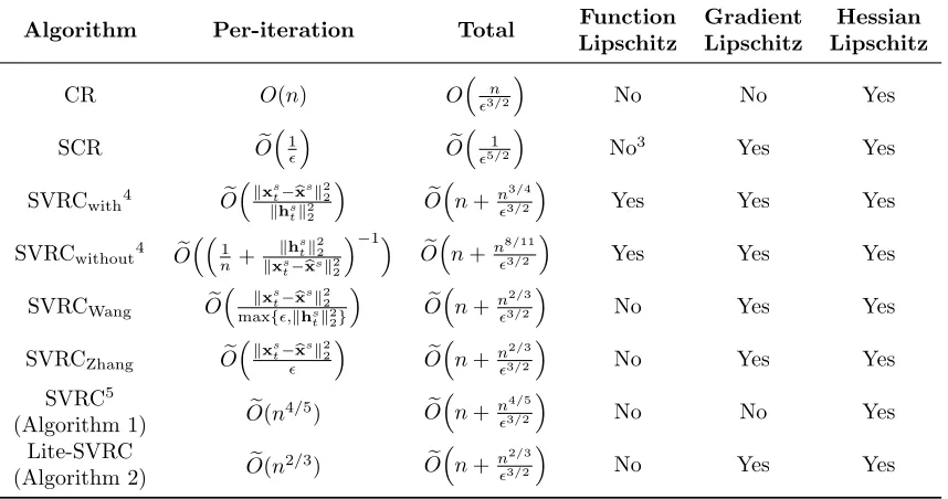
Remark 21 Note that the CSO oracle complexity of Lite-SVRC is the same as SVRC. In what follows, we present a comprehensive comparison on Hessian sample complexity between our Lite-SVRC and other related algorithms in Table 2. The algorithm proposed in Wang et al. (2018a) has two versions: sample with replacement and sample without replacement. For the completeness, we present both versions in Wang et al. (2018a). From Table 2 we can

see that Lite-SVRC strictly outperforms CR by a factor of n1/3 and outperforms SVRC by

a factor of n2/15 in terms of Hessian sample complexity. Lite-SVRC also outperforms SCR

when = O(n−2/3), which suggests that the variance reduction scheme makes Lite-SVRC

perform better in the high accuracy regime. More importantly, our proposed Lite-SVRC does

(14)

the algorithm proposed in Wang et al. (2018a). In terms of Hessian sample complexity, our

algorithm directly improves that of Wang et al. (2018a) by a factor of n2/33. The Hessian

sample complexity of Lite-SVRC is the same as that of the algorithms recently proposed in Wang et al. (2018b) and Zhang et al. (2018). Nevertheless, Lite-SVRC uses a constant Hessian sample batch size in contrast to the adaptive batch size as used in Wang et al. (2018b); Zhang et al. (2018), which makes the use of Lite-SVRC algorithm much simpler and more practical.

Algorithm Per-iteration Total Function Gradient Hessian Lipschitz Lipschitz Lipschitz

CR O(n) O n

3/2

No No Yes

SCR Oe

1

e O 1

5/2

No3 _Yes _Yes

SVRCwith4 Oe _k_xs

t−bx

s_k2 2 khs

tk22

e

On+n33//24

Yes Yes Yes

SVRCwithout4 Oe

1

n+

khs tk22 kxs

t−bx

s_k2 2

−1 e

On+n83//112

Yes Yes Yes

SVRCWang Oe _k_xs

t−bx

s_k2 2 max{,khs

tk22}

e

On+n32//23

No Yes Yes

SVRCZhang Oe

_k_xs t−bx

s_k2 2

e

On+n32//23

No Yes Yes

SVRC5

e

O(n4/5) Oe

n+n34//25

No No Yes

(Algorithm 1) Lite-SVRC

e O(n2/3₎

e

On+n32//23

No Yes Yes

(Algorithm 2)

Table 2: Comparisons of per-iteration and total sample complexities of Hessian evaluations for different algorithms: CR (Nesterov and Polyak, 2006), SCR (Kohler and Luc-chi, 2017; Xu et al., 2017a), SVRCwith (Wang et al., 2018a), SVRCwithout (Wang et al., 2018a), SVRCWang (Wang et al., 2018b), SVRCZhang (Zhang et al., 2018), SVRC (Algorithm 1) and Lite-SVRC (Algorithm 2). Similar to Table 1, the CSO oracle complexities of all the methods being compared are the same, i.e. O(1/3/2). Therefore, we omit it for simplicity.

Recall the inexact cubic subproblem solver defined in Section 5. The same inexact CSO oracles can also be used in Algorithm 2. In what follows, we present the convergence result of Lite-SVRC with inexact CSO oracles.

3. Although the refined SCR in Xu et al. (2017b) does not need function Lipschitz, the original SCR in Kohler and Lucchi (2017) needs it.

4. In Wang et al. (2018a), both algorithms need to calculate λmin(∇2F(xst)) at each iteration to decide

whether the algorithm should continue, which adds additional O(n) Hessian sample complexity. We

choose not to include this into the results in the table.

(15)

Theorem 22 Suppose that for each s, t, ehs_t is an inexact solver of cubic subproblem ms_t(h)

satisfying Condition 11. Then under the same conditions of Theorem 18, the output of Algorithm 2 satisfies

E[µ(xout)]≤

216C2

ML

1/2 2 ∆F

ST + 432C 2

ML

1/2

2 δ. (24)

In addition, Algorithm 2 with inexact oracle can also reduce the Hessian sample com-plexity, which is summarized in the following corollary.

Corollary 23 Suppose that for eachs, t,hes_t is an inexact solver of cubic subproblem ms_t(h)

satisfying Condition 11 with δ = (864C_M2 L₂1/2)−13/2. Then with the same choice of

pa-rameters in Corollary 20, Algorithm 2 will find an (,√L2)-approximate local minimum

within

e O

n+∆F

√

L2 3/2 ·n

2/3

stochastic Hessian evaluations,

and

O

∆F

√

L2 3/2

CSO calls.

8. Experiments

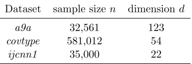
In this section, we conduct experiments on real world datasets to support our theoretical analysis of the proposed SVRC and Lite-SVRC algorithms. We investigate two nonconvex problems on three different datasets,a9a,ijcnn1 andcovtype, which are all common datasets used in machine learning and the sizes are summarized in Table 3.

8.1. Baseline Algorithms

Dataset sample size n dimension d

a9a 32,561 123

covtype 581,012 54

ijcnn1 35,000 22

Table 3: Datasets used in experiments. To validate the superior performance of

the proposed SVRC (Algorithm 1) in terms of second-order oracles, we com-pare it with the following baseline algo-rithms: (1) trust-region Newton meth-ods (TR) (Conn et al., 2000); (2) Adap-tive Cubic regularization (Cartis et al., 2011a,b); (3) Subsampled Cubic regular-ization (Kohler and Lucchi, 2017); (4) Gradient Cubic regularization (Carmon and Duchi, 2016) and (5) Stochastic

(16)

et al. (2018a), but the one based on sampling without replacement performs better in both theory and experiments. We therefore only compare with this one. Note that the SVRC algorithms in Wang et al. (2018b); Zhang et al. (2018) are essentially the same as our Lite-SVRC algorithm, except in the choice of batch size for stochastic Hessian. Thus we do not compare our Lite-SVRC with these algorithms (Wang et al., 2018b; Zhang et al., 2018).

8.2. Implementation Details

For Subsampled Cubic and SVRC-without, the sample size Bk is dependent on khkk2 (Kohler and Lucchi, 2017) and Bh is dependent on khstk2 (Wang et al., 2018a), which make these two algorithms implicit algorithms. To address this issue, we follow the sug-gestion in Kohler and Lucchi (2017); Wang et al. (2018a) and use khk−1k2 and khst−1k2 instead ofkhkk2 andkhstk2. Furthermore, we choose the penalty parameterMs,tfor SVRC,

SVRC-without and Lite-SVRC as constants which are suggested by the original papers of these algorithms. Finally, to solve the CR sub-problem in each iteration, we choose to solve the sub-problem approximately in the Krylov subspace spanned by Hessian related vectors, as used by Kohler and Lucchi (2017).

8.3. Nonconvex Optimization Problems

In this subsection, we formulate the nonconvex optimization problems that will be studied in our experiments. In particular, we choose two nonconvex regression problem as our objectives with the following nonconvex regularizer

g(λ, γ,x) =λ·

d

X

i=1

(γxi)2

1 + (γxi)2

, (25)

where λ, γ are the control parameters andxi is the i-th coordinate of x. λ and γ are set

differently for each dataset. This regularizer has been widely used in nonconvex regression problem, which can be regarded as a special example of robust nonlinear regression (Reddi et al., 2016b; Kohler and Lucchi, 2017; Wang et al., 2018a).

8.3.1. Logistic Regression with Nonconvex Regularizer

The first problem is a binary logistic regression problem with a nonconvex regularizer g (Reddi et al., 2016b). Given training data xi ∈ Rd and label yi ∈ {0,1}, 1 ≤ i≤ n, our

goal is to solve the following optimization problem:

min

s∈Rd

1 n

n

X

i=1

yi·logφ(s>xi) + (1−yi)·log[1−φ(s>xi)]

+g(λ, γ,s), (26)

whereφ(x) = 1/(1 + exp(−x)) is the sigmoid function and g is defined in (25).

8.3.2. Nonlinear Least Square with Nonconvex Regularizer

(17)

Given training dataxi∈Rdandyi ∈ {0,1}, 1≤i≤n, our goal is to minimize the following

problem

min

s∈_Rd

1 n

n

X

i=1

yi−φ(s>xi)2+g(λ, γ,s). (27)

Here φ(x) = 1/(1 + exp(−x)) is again the sigmoid function andg is defined in (25).

8.4. Experimental Results for SVRC

In this subsection, we present the experimental results for SVRC compared with baseline algorithms (1)-(5) listed in Section 8.1. Here, we fix λ= 10 and γ = 1 of the nonconvex regularizergin (25) for both the logistic regression and the nonlinear least square problems.

Calculation for SO calls: ForSubsampled Cubic, each loop takes (Bg+Bh) SO calls,

whereBg and Bh are the subsampling sizes of gradient and Hessian. ForStochastic Cubic,

each loop costs (ng+nh) SO calls, wherengandnhdenote the subsampling sizes of gradient

and Hessian-vector operator. Gradient Cubic, Adaptive Cubic and TR cost n SO calls in each loop. We define the amount of epochs to be the amount of SO calls divided byn.

Parameters: For each algorithm and each dataset, we choose different bg, bh, T for

the best performance. Meanwhile, we choose the cubic regularization parameter as Ms,t=

α/(1 +β)(s+t/T),α,β >0 for each iteration. Whenβ= 0, it has been proved to enjoy good convergence performance. This choice of parameter is similar to the choice of penalty pa-rameter inSubsampled CubicandAdaptive Cubic, which sometimes makes some algorithms behave better in our experiments.

Subproblem Solver: With regard to the cubic subproblem solver for solving (7), we choose the Lanczos-type method used in Cartis et al. (2011a), which finds the global minimizerhs_t of ms_t(h) in a Krylov subspaceK_l= span{v_ts,Us_tv_ts,(Us_t)2v_ts, . . . ,(Us_t)l−1v_ts}, whereldis the dimension ofK_land can be selected manually or adaptively (Cartis et al., 2011a; Kohler and Lucchi, 2017). The computational complexity of Lanczos-type method consists of two parts according to Carmon and Duchi (2018). First, (l−1) matrix-vector products are performed to calculate the basis of K_l, whose computational complexity is O(d2_{l). Second, the minimizer of}_ms

t(h) is computed in subspace Kl, whose computational

complexity isO(llogl). Thus, the total computational complexity of Lanczos-type method isO(d2l).

At each iteration, SVRC needs to compute the semi-stochastic gradientvs_t and Hessian

Us_t, which costs O(dbg+d2bh) computational complexity for both nonconvex regularized

logistic regression and nonlinear least square problems, wherebg and bh are the mini-batch

sizes of stochastic gradient and Hessian respectively. Putting these pieces together, the per-iteration complexity of SVRC isO(dbg+d2bh+d2l), and the total computational complexity

of SVRC is O(ST(dbg+d2bh+d3)), where S is the number of epochs and T is the length

of epoch.

For the binary logistic regression problem in (26), the parameters of Ms,t = α/(1 +

β)(s+t/T), α, β > 0 are set as follows: α = 0.05, β = 0 for a9a and ijcnn1 datasets and α = 5e3, β = 0.15 for covtype. The experimental results are shown in Figure 1. For the non-linear least squares problem in (27), we set α = 0.05,1e8,0.003 and β = 0,1,0.5 for

(18)

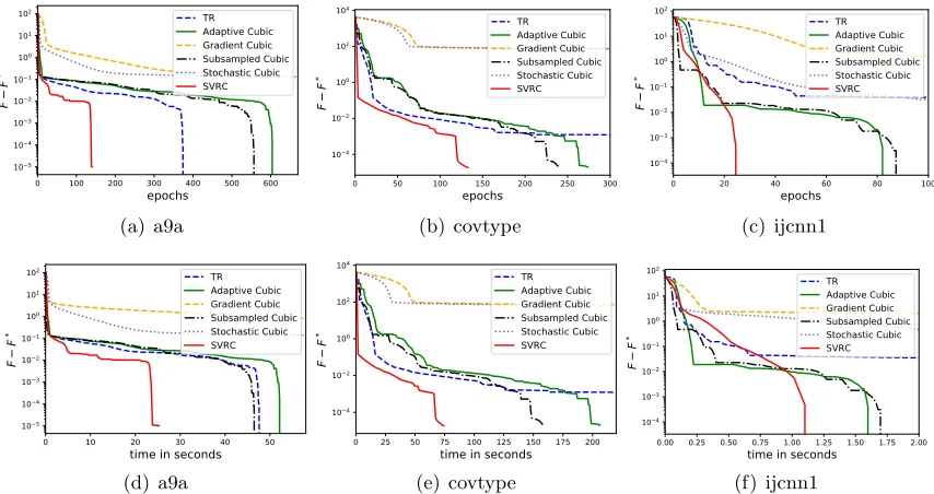
2. From both Figures 1 and 2, we can see that SVRC outperforms all the other baseline algorithms on all the datasets. The only exception happens in the non-linear least square problem on the covtype dataset, where our algorithm behaves a little worse than Adaptive Cubic at the high accuracy regime in terms of epoch counts. However, under this setting, our algorithm still outperforms the other baselines in terms of the CPU time.

0 100 200 300 400 500 600 epochs

105

104

103

102

101

100

101

102

F

*

TR Adaptive Cubic Gradient Cubic Subsampled Cubic Stochastic Cubic SVRC

(a) a9a

0 50 100 150 200 250 300 epochs

104 102 100 102 104

F

*

(b) covtype

0 20 40 60 80 100 epochs

104 103 102 101 100 101 102

F

*

(c) ijcnn1

0 10 20 30 40 50 time in seconds 105

104

103

102

101

100

101

102

F

*

(d) a9a

0 25 50 75 100 125 150 175 200 time in seconds 104

102

100

102

104

F

*

(e) covtype

0.00 0.25 0.50 0.75 1.00 1.25 1.50 1.75 2.00 time in seconds

104 103 102 101 100 101 102

F

*

(f) ijcnn1

Figure 1: Logarithmic function value gap for nonconvex regularized logistic regression on different datasets. (a), (b) and (c) present the oracle complexity comparison; (d), (e) and (f) present the runtime comparison.

8.5. Experimental Results for Lite-SVRC

In this subsection, we present the experimental results for Lite-SVRC compared with all the baselines listed in Section 8.1. For Lite-SVRC, we use the same cubic subproblem solver used for SVRC in the previous subsection.

In the binary logistic regression problem in (26), for the nonconvex regularizergin (25), we set λ= 10−3 for all three datasets, and set γ = 10,50,100 for a9a,ijcnn1 and covtype

(19)

0 10 20 30 40 50 60 70 80 epochs 105 104 103 102 101 100 F F * TR Adaptive Cubic Gradient Cubic Subsampled Cubic Stochastic Cubic SVRC (a) a9a

0 10 20 30 40 50 epochs 105 104 103 102 101 F F * TR Adaptive Cubic Gradient Cubic Subsampled Cubic Stochastic Cubic SVRC (b) covtype

0 5 10 15 20 25 30 epochs 105 104 103 102 101 F F * TR Adaptive Cubic Gradient Cubic Subsampled Cubic Stochastic Cubic SVRC (c) ijcnn1

0 1 2 3 4 5 6 7 time in seconds

105 104 103 102 101 100 F F * TR Adaptive Cubic Gradient Cubic Subsampled Cubic Stochastic Cubic SVRC (d) a9a

0 5 10 15 20 25 30 35 40 time in seconds

105 104 103 102 101 F F * TR Adaptive Cubic Gradient Cubic Subsampled Cubic Stochastic Cubic SVRC (e) covtype

0.00 0.05 0.10 0.15 0.20 0.25 0.30

time in seconds

105 104 103 102 101 F F * TR Adaptive Cubic Gradient Cubic Subsampled Cubic Stochastic Cubic SVRC (f) ijcnn1

Figure 2: Logarithmic function value gap for nonlinear least square on different datasets. (a), (b) and (c) present the oracle complexity comparison; (d), (e) and (f) present the runtime comparison.

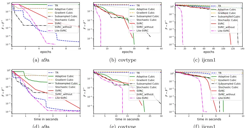
0 50 100 150 200 250 300 350 400 450 epochs 105 104 103 102 101 100 101 102 F F * TR Adaptive Cubic Gradient Cubic Subsampled Cubic Stochastic Cubic SVRC SVRC_without Lite-SVRC (a) a9a

0 10 20 30 40 50 60 70 epochs 105 104 103 102 101 F F * TR Adaptive Cubic Gradient Cubic Subsampled Cubic Stochastic Cubic SVRC SVRC_without Lite-SVRC (b) covtype

0 20 40 60 80 100 epochs 103 102 101 100 101 102 F F * TR Adaptive Cubic Gradient Cubic Subsampled Cubic Stochastic Cubic SVRC SVRC_without Lite-SVRC (c) ijcnn1

0 20 40 60 80 100 120 140 time in seconds

105 104 103 102 101 100 101 102 F F * TR Adaptive Cubic Gradient Cubic Subsampled Cubic Stochastic Cubic SVRC SVRC_without Lite-SVRC (d) a9a

0 5 10 15 20 25 30 35 40 time in seconds

105 104 103 102 101 F F * TR Adaptive Cubic Gradient Cubic Subsampled Cubic Stochastic Cubic SVRC SVRC_without Lite-SVRC (e) covtype

0.00 0.25 0.50 0.75 1.00 1.25 1.50 1.75 2.00 time in seconds 103 102 101 100 101 102 F F * TR Adaptive Cubic Gradient Cubic Subsampled Cubic Stochastic Cubic SVRC SVRC_without Lite-SVRC (f) ijcnn1

(20)

0 2 4 6 8 10 epochs

105 104 103 102 101 100

F

*

TR Adaptive Cubic Gradient Cubic Subsampled Cubic Stochastic Cubic SVRC SVRC_without Lite-SVRC

(a) a9a

0 10 20 30 40 50 epochs

105 104 103 102

F

*

(b) covtype

0 20 40 60 80 100 120 140 epochs

105 104 103 102 101 100

F

*

(c) ijcnn1

0 1 2 3 4 5

time in seconds 105

104

103

102

101

100

F

*

(d) a9a

0 5 10 15 20 25 30 time in seconds

105 104 103 102

F

*

(e) covtype

0 2 4 6 8 10

time in seconds 105

104 103 102 101 100

F

*

(f) ijcnn1

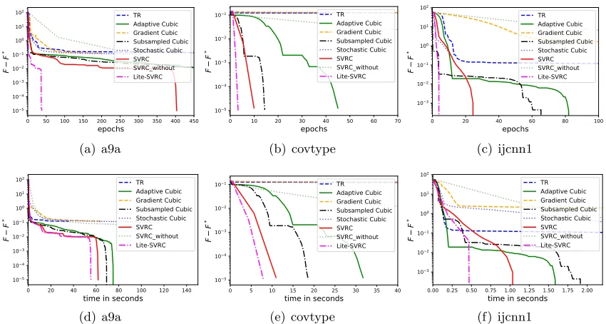
Figure 4: Function value gap of different algorithms for nonlinear least square problems on different datasets. (a)-(c) are plotted w.r.t. Hessian sample complexity. (d)-(e) are plotted w.r.t. CPU runtime.

than other methods, because as we pointed out in the introduction, it needs to compute the minimum eigenvalue of the Hessian in each iteration, which actually makes the Hessian sample complexity even worse than Subsampled Cubic, let alone the runtime complexity.

For the least square problem in (27), the parametersλandγin the nonconvex regularizer for different datasets are set as follows: λ= 5×10−3 for all three datasets, andγ = 10,20,50

fora9a,ijcnn1 andcovtype datasets respectively. The experimental results are summarized

in Figure 4, where the first row shows the plots of function value gap v.s. Hessian sample complexity and the second row presents the plots of function value gap v.s. CPU runtime (in seconds). It can be seen that Lite-SVRC again achieves the best performance among all the algorithms regarding to both sample complexity of Hessian and runtime when the required precision is high, which supports our theoretical analysis.

9. Conclusions

(21)

Acknowledgement

We would like to thank the anonymous reviewers for their helpful comments. This research was sponsored in part by the National Science Foundation IIS-1904183 and IIS-1906169. The views and conclusions contained in this paper are those of the authors and should not be interpreted as representing any funding agencies.

Appendix A. Proof of Main Theoretical Results for SVRC

In this section, we present the proofs of our main theoretical results for SVRC. Let us first recall the notations used in Algorithm 1. vs_t and Us_t are the semi-stochastic gradient and Hessian defined in (5) and (6) respectively. xs_t’s are the iterates and _bxs’s are the reference points used in Algorithm 1. bg and bh are the batch sizes of semi-stochastic gradient and

Hessian. S and T are the number of epochs and epoch length of Algorithm 1. We set Ms,t :=M =CML2 as suggested by Theorems 6 and 13, where CM >0 is a constant. hst

is the exact minimizer ofms_t(h), wherem_ts(h) is defined in (7). ehs_t is the inexact minimizer defined in (15).

In order to prove Theorems 6 and 13, we lay down the following useful technical lemmas. The first lemma is standard in the analysis cubic regularization methods.

Lemma 24 Suppose F is L2-Hessian Lipschitz for some constant L2 > 0. For the

semi-stochastic gradient and Hessian defined in (5)and (6), we have the following results:

vs_t +Us_ths_t +M 2 kh

s

tk2hst = 0, (28)

Us_t +M 2 kh

s

tk2I0, (29)

hvs_t,hs_ti+1 2hU

s

thst,hsti+

M 6 kh

s tk32≤ −

M 12kh

s

tk32. (30)

The next two important lemmas control the variances ofv_ts andUs_t.

Lemma 25 For the semi-stochastic gradient vs_t defined in (5), we have

Eitk∇F(x

s

t)−vtsk

3/2

2 ≤

L3₂/2 b3g/4

kxs_t−x_bsk3₂,

where Eit is the expectation over all it∈Ig.

Lemma 26 Let Us_t be the semi-stochastic Hessian defined in (6). If the batch size satisfy

bh ≥400 logd, then we have

Ejt

∇2F(xs_t)−Us_t 3

2≤1200L 3 2

logd

bh

3/2

kxs_t −_bxsk3₂,

(22)

Lemma 27 For the semi-stochastic gradient and Hessian defined in (5) and (6) and h ∈

Rd, we have

h∇F(xs_t)−vs_t,hi ≤ M

27khk 3 2+

2k∇F(xs_t)−v_tsk3₂/2

M1/2 ,

∇2F(xs_t)−Us_t

h,h

≤ 2M

27 khk 3 2+

27 M2

∇2F(xs_t)−Us_t 3 2.

Lemma 28 Let h ∈ _Rd _and _C

M ≥ 100. For the semi-stochastic gradient and Hessian

defined in (5)and (6), we have

µ(xs_t+h)≤9C_M3/2 h

M3/2khk3₂+k∇F(xs_t)−vs_tk₂3/2+M−3/2∇2F(xs_t)−Us_t 3 2 +k∇ms_t(h)k3₂/2+M3/2khk₂− khs_tk₂

3i .

Lemma 29 Leth∈_Rd _and_C_≥_3/2_{, For the semi-stochastic gradient and Hessian defined}

in (5) and (6), we have

kxs_t+h−x_bsk3₂≤2C2khk3₂+ (1 + 3/C)kxs_t−_bxsk3₂. (31)

Lemma 30 We define constant series ct for 0 ≤ t ≤ T as follows: cT = 0 and ct =

ct+1(1 + 3/T) +M(500T3)−1 for 0≤t≤T −1. Then we have for any 1≤t≤T,

M/24−2ctT2 ≥0. (32)

A.1. Proof of Theorem 6

Proof [Proof of Theorem 6] We first upper bound F(xs_t₊₁) as follows F(xs_t₊₁)≤F(xs_t) +h∇F(xs_t),hs_ti+1

2

∇2F(xs_t)hs_t,hs_t+L2 6 kh

s tk32 =F(xs_t) +hv_ts,hs_ti+1

2hU

s

thst,hsti+

M 6 kh

s

tk32+h∇F(xts)−vst,hsti

+1 2

∇2F(xs_t)−Us_ths_t,hs_t−M −L2

6 kh

s tk32

≤F(xs_t)−M

12kh

s tk32+

M 27kh

s tk32+

2k∇F(xs_t)−vs_tk3₂/2

M1/2

+1 2

2M

27 kh

s tk32+

27 M2

∇2F(xs_t)−Us_t 3 2

−M−L2

6 kh

s tk32

≤F(xs_t)−M

12kh

s tk32+

2

M1/2k∇F(x

s

t)−vstk

3/2 2 +

27 M2

∇2F(xs_t)−Us_t 3

2, (33) where the first inequality follows from Lemma 40 and the second inequality holds due to Lemmas 24 and 27. We define

Rs_t =EF(xts) +ctkxst−xb

s_k3 2

(23)

wherect is defined in Lemma 30. Then by Lemma 29, for T ≥3/2 we have

ct+1kxst+1−xb

s_k3

2 =ct+1khst+xst−xb

s_k3

2 ≤2ct+1T2khstk23+ct+1(1 + 3/T)kxst−bx

s_k3 2. (35) Applying Lemma 28 withh=hs_t, we have

240C_M2 L1₂/2−1µ(xs_t₊₁)≤ M

24kh

s tk32+

k∇F(xs_t)−vs_tk3₂/2

24M1/2 +

∇2F(xs_t)−Us_t 3 2 24M2 +k∇m

s t(hst)k

3/2 2 24M1/2 +

M 24

khs_tk₂− khs_tk₂ 3

= M 24kh

s tk32+

24M1/2 +

∇2F(xs_t)−Us_t 3 2

24M2 , (36) where the equality is due to Lemma 24. Adding (33) with (35) and (36) and taking total expectation, we have

Rs_t₊₁+ 240C_M2 L1₂/2−1

E[µ(xst+1)] =E

h

F(xs_t₊₁) +ct+1kxst+1−bx

s_k3

2+ 240CM2 L

1/2 2

−1

µ(xs_t₊₁)i

≤_E

F(xs_t) +ct+1(1 + 3/T)kxst−xb

s_k3

2− khstk32 M/24−2ct+1T2

+E

h

3M−1/2k∇F(x_ts)−vs_tk₂3/2+ 28M−2∇2F(xs_t)−Us_t 3 2 i

≤EF(xst) +ct+1(1 + 3/T)kxst−xb

s_k3 2

+E

h

3M−1/2k∇F(x_ts)−vs_tk3₂/2

+ 28M−2∇2F(xs_t)−Us_t 3 2 i

, (37)

where the third inequality holds due to Lemma 30. To further bound (37), we have

3

M1/2Ek∇F(x

s

t)−vtsk

3/2

2 ≤

3L3₂/2 M1/2_b3/4

g

Ekxst−bx

s_k3 2 ≤

M 1000T3Ekx

s t −bx

s_k3

2, (38) where the first inequality holds due to Lemma 25, the second inequality holds due toM ≥

100L2 and bg ≥5T4 from the condition of Theorem 6. We also have

28 M2E

∇2F(xs_t)−Us_t 3 2≤

28×15000L3₂ M2_(b

h/logd)3/2

Ekxst−bx

s_k3 2 ≤

M 1000T3Ekx

s t −xb

s_k3

2, (39) where the first inequality holds due to Lemma 26, where we have bh ≥ 100T2logd ≥

400 logd, and the second inequality holds due toM ≥100L2 and bh≥100T2logdfrom the

assumption of Theorem 6. Thus, submitting (38) and (39) into (37), we have

Rs_t₊₁+ 240C_M2 L1₂/2−1E[µ(xst+1)]≤E

F(xs_t) +kxs_t−x_bsk3₂

ct+1(1 + 3/T) + M 500T3

=EF(xst) +ctkxst−bx

s_k3 2

(24)

where the first equality holds due to the definition of ct in Lemma 30. Telescoping (40)

from t= 0 to T −1, we have

Rs₀−R_Ts ≥

T

X

t=1

240C_M2 L1₂/2−1E[µ(xst)].

By the definition of cT in Lemma 30, we have cT = 0, then Rs_T = EF(xsT) +cTkxsT −

b

xsk3 2

= EF(xb

s+1_{); meanwhile by the definition of} _xs

0, we have xs0 = xb

s_{. Thus we have}

Rs

0 =E

F(xs

0) +c0kxs0−bx

s_k3 2

=EF(bx

s_{), which implies}

EF(xb

s₎₋ EF(xb

s+1_{) =}_Rs

0−RsT ≥ 240CM2 L

1/2 2

−1

T

X

t=1

E[µ(xst)]. (41)

Finally, telescoping (41) froms= 1 to S yields

∆F ≥ S

X

s=1

EF(bx

s₎₋ EF(bx

s+1₎_≥ _240C2

ML

1/2 2

−1

S

X

s=1

T

X

t=1

E[µ(xst)].

By the definition about choice of xout, we complete the proof.

A.2. Proof of Corollary 9

Proof We can verify that the parameter setting in Corollary 9 satisfies the requirement of Theorem 6. Thus, submitting the choice of parameters into Theorem 6, the output of Algorithm 1xout satisfies that

E[µ(xout)]≤ 240C

2

ML

1/2 2 ∆F

ST ≤

3/2_, ₍₄₂₎

which indeed implies that xout is an (,

√

L2)-approximate local minimum. Next we cal-culate how many SO calls and CSO calls are needed. Algorithm 1 needs to calcal-culate full gradient gs and full Hessian Hs at the beginning of each epoch, with n SO calls. In each

epoch, Algorithm 1 needs to calculate v_ts and Us_t with bg +bh SO calls at each iteration.

Thus, the total amount of SO calls is

Sn+ (ST)(bg+bh)≤n+C1∆FL1₂/2n4/5−3/2+C1∆FL1₂/2−3/2(5n4/5+ 1000n2/5logd)

=Oe

n+∆F

√

L2n4/5 3/2

,

where C1 = 240C_M2 . For the CSO calls, Algorithm 1 needs to solve cubic subproblem at each single iteration. Thus, the total amount of CSO calls is

ST ≤C1∆FL12/2

−3/2₌_O

∆F

√

L2 3/2

(25)

A.3. Proof of Theorem 13

Proof [Proof of Theorem 13] Similar to (33) in the proof of Theorem 6, we have

F(xs_t₊₁)≤F(x_ts) +∇F(xs_t),hes_t

+ 1 2

∇2F(xs_t)hes_t,hes_t

+L2 6

ehs_t

3 2 =F(xs_t) +vs_t,hes_t

+1

2

Us_thes_t,ehs_t

+M 6

ehs_t

3 2+

∇F(xs_t)−vs_t,ehs_t

+1 2

(∇2F(xs_t)−U_ts)hes_t,ehs_t

−M−L2

6 ehs_t

3 2

≤F(xs_t)−M

12 ehs_t

3 2+δ+

M 27 ehs_t

3 2+

2k∇F(xs_t)−vs_tk3₂/2

M1/2

+1 2 2M 27 ehs_t

3 2+ 27 M2

∇2F(xs_t)−Us_t 3 2

−M−L2

6 ehs_t

3 2

≤F(xs_t)−M

12 ehs_t

3 2+

2

M1/2k∇F(x

s

t)−vstk

3/2 2 +

27 M2

∇2F(xs_t)−Us_t 3 2+δ,

(43)

where the second inequality holds because hes_t is an inexact solver satisfying Condition 11. By Lemma 29 withh=hes_t, we have

ct+1kxst+1−bx

s_k3 2=ct+1

xs_t−_bxs+hes_t 3

2≤2ct+1T 2

ehs_t 3

2+ct+1(1 + 3/T)kx

s t −bx

s_k3 2.

(44)

By Lemma 28, we also have

240C_M2 L1₂/2−1µ(xs_t₊₁) = 240C_M2 L1₂/2−1

µ xs_t +hes_t

≤ M

24 ehs_t

3 2+

24M1/2 +

∇2F(xs_t)−Us_t 3 2 24M2 +

∇ms_t hes_t

3/2 2 24M1/2 +

M ehs_t

2− kh

s tk2

3 24 ,

(45)

Since ehs_t is an inexact solver satisfying Condition 11, we have

∇ms_t hes_t

3/2 2 24M1/2 +

M ehs_t

2− kh

s tk2

3 24 ≤ δ 24 + δ

24 < δ. (46)

Submitting (46) into (45), we have

240C_M2 L1₂/2−1µ(xs_t₊₁)≤ M

24 ehs_t

3 2+

24M1/2 +

∇2F(xs_t)−Us_t 3 2

24M2 +δ. (47) Then adding (43), (44) and (47) up, we have

Rs_t₊₁+ 240C_M2 L₂1/2−1E[µ(xst+1)] =E

h

F(xs_t₊₁) +ct+1kxst+1−xb

s_k3

2+ 240CM2 L

1/2 2

−1

(26)

≤_EhF(xs_t) +ct+1(1 + 3/T)kxst−bx

s_k3 2−

ehs_t

3

2 M/24−2ct+1T 2i +E

3

M1/2k∇F(x

s

t)−vstk

3/2 2 +

28 M2

∇2F(xs_t)−Us_t 3 2 + 2δ ≤_E

F(xs_t) +ct+1(1 + 3/T)kxst−bx

s_k3 2

+E

3

M1/2k∇F(x

s

t)−vstk

3/2 2 +

28 M2

∇2F(xs_t)−Us_t 3 2

+ 2δ. (48)

Since the parameter setting is the same as Theorem 6, by (38) and (39), we have

3

M1/2Ek∇F(x

s

t)−vstk

3/2 2 ≤

M 1000T3Ekx

s t−xb

s_k3

2, (49)

28 M2E

∇2F(xs_t)−Us_t 3 2≤

M 1000T3Ekx

s t−xb

s_k3

2. (50)

Submitting (49) and (50) into (48) yields

R_ts₊₁+ 240C_M2 L1₂/2−1E[µ(xst+1)]≤E

F(xs_t) +kxs_t−_bxsk3₂

ct+1(1 + 3/T) +

M 500T3

+ 2δ

=EF(xst) +ctkxst−xb

s_k3 2

+ 2δ

=Rs_t+ 2δ, (51)

where the first equality holds due to the definition of ct in Lemma 30. Telescoping (40)

from t= 0 to T −1, we have

Rs₀−Rs_T ≥

T

X

t=1

240C_M2 L1₂/2−1E[µ(xst)]−2δ

.

By the definition of cT in Lemma 30, we have cT = 0, then RsT = E

F(xs_T) +cTkxsT −

b

xs_k3 2

= E[F(bx

s+1_{)]; meanwhile by the definition of} _xs

0, we have xs0 = bx

s_{. Thus we have}

R₀s=EF(x0s) +c0kxs0−bx

s_k3 2

=E[F(xb

s_{)], which further implies}

E[F(xb

s_)]₋ E[F(xb

s+1_{)] =}_Rs

0−RsT ≥ T

X

t=1

240C_M2 L1₂/2−1E[µ(xst)]−2δ

. (52)

Finally, telescoping (52) froms= 1 to S, we obtain

∆F ≥ S

X

s=1

E[F(bx

s_)]₋ E[F(xb

s+1_)]_≥

S X s=1 T X t=1 h

240C_M2 L1₂/2−1

E[µ(xst)]−2δ

i .

(27)

A.4. Proof of Corollary 15

Proof [Proof of Corollary 15] Under the parameter choice in Corollary 15, it holds that

E[µ(xout)]≤

240C_M2 L1₂/2∆F

ST + 480C 2

ML

1/2 2 δ≤

3/2_{/2 +}3/2_{/2 =}3/2_. ₍₅₃₎ Thus, xout is an (,

√

L2)-approximate local minimum. By the proof of Corollary 9, the total amount of SO calls is

Sn+ (ST)(bg+bh)≤n+C1∆FL12/2n

4/5−3/2₊_C

1∆FL12/2

−3/2_(5n4/5_{+ 1000n}2/5_log_d) =Oe

n+∆F

√

L2n4/5 3/2

,

where C1 = 480CM2 . For the CSO calls, Algorithm 1 needs to solve cubic subproblem at

each single iteration. Thus, the total amount of CSO calls is

ST ≤C1∆FL12/2

−3/2₌_O

∆F

√

L2 3/2

.

Appendix B. Proof of Technical Lemmas in Appendix A

In this section, we prove the technical lemmas used in Appendix A.

B.1. Proof of Lemma 24

The result of Lemma 24 is typical in the literature of cubic regularization (Nesterov and Polyak, 2006; Cartis et al., 2011a,b), but no exactly the same result has been shown in any formal way. Thus we present the proof here for self-containedness.

Proof [Proof of Lemma 24] For simplicity, we let g =v_ts,H=U_ts, θ=Mt and hopt =hst.

Then we need to prove

g+Hhopt+ θ

2khoptk2hopt=0, (54)

H+ θ

2khoptk2I0, (55)

hg,hopti+ 1

2hHhopt,hopti+ θ 6khoptk

3 2≤ −

θ

12khoptk 3

2. (56)