Kernel Approximation Methods for Speech Recognition
Avner May1† [email protected]
Alireza Bagheri Garakani2‡ [email protected]
Zhiyun Lu2‡ [email protected]
Dong Guo2‡ [email protected]
Kuan Liu2,5‡ [email protected]
Aur´elien Bellet3
Linxi Fan1 [email protected]
Michael Collins4,5 [email protected]
Daniel Hsu4
Brian Kingsbury6 [email protected]
Michael Picheny6 [email protected]
Fei Sha2
1Department of Computer Science, Stanford University, Stanford, CA 94305, USA
2Department of Computer Science, University of Southern California, Los Angeles, CA 90089, USA 3INRIA, 40 Avenue Halley, 59650 Villeneuve d’Ascq, France
4Department of Computer Science, Columbia University, New York, NY 10027, USA 5Google Inc, USA
6IBM Research AI, Yorktown Heights, NY 10598, USA
† ‡: Contributed equally as the first and second co-authors, respectively
Editor:Benjamin Recht
Abstract
We study the performance of kernel methods on the acoustic modeling task for automatic speech recognition, and compare their performance to deep neural networks (DNNs). To scale the kernel methods to large data sets, we use the random Fourier feature method of Rahimi and Recht (2007). We propose two novel techniques for improving the perfor-mance of kernel acoustic models. First, we propose a simple but effective feature selection method which reduces the number of random features required to attain a fixed level of performance. Second, we present a number of metrics which correlate strongly with speech recognition performance when computed on the heldout set; we attain improved perfor-mance by using these metrics to decide when to stop training. Additionally, we show that the linear bottleneck method of Sainath et al. (2013a) improves the performance of our kernel models significantly, in addition to speeding up training and making the models more compact. Leveraging these three methods, the kernel methods attain token error rates between 0.5% better and 0.1% worse than fully-connected DNNs across four speech recognition data sets, including the TIMIT and Broadcast News benchmark tasks.
Keywords: kernel methods, deep neural networks, acoustic modeling, automatic speech recognition, feature selection, logistic regression
c
1. Introduction
Large-scale non-linear classification is an important and challenging problem in machine learning. In recent years, deep learning techniques have significantly advanced state-of-the-art performance on classification problems in various domains, including automatic speech recognition (ASR) (Seide et al., 2011a; Hinton et al., 2012; Mohamed et al., 2012; Xiong et al., 2017; Saon et al., 2017), computer vision (Krizhevsky et al., 2012; Simonyan and Zisserman, 2015; He et al., 2016), and natural language processing (NLP) (Mikolov et al., 2013; Sutskever et al., 2014; Andor et al., 2016). Deep neural networks (DNNs) are able to gracefully scale to large data sets, and can successfully leverage this additional data to achieve strong empirical performance. In contrast, kernel methods, which are attractive due to their high capacity, as well as for their theoretical learning guarantees and tractability (Sch¨olkopf and Smola, 2002), do not scale well. In particular, with data sets of sizeN, the Θ(N2) size of the kernel matrix makes training prohibitively slow, while the typical Θ(N) size of the resulting models (Steinwart, 2003) makes their deployment impractical.
An important technique for scaling kernel methods to large data sets is to use approxi-mation. Kernel approximation methods construct explicit feature maps whose dot-products approximate the kernel function, and then learn linear models with these features. Notable approximation methods include the Nystr¨om method (Williams and Seeger, 2000), and ran-dom Fourier features (RFFs) (Rahimi and Recht, 2007). Although these methods make it possible to apply kernel methods to large-scale tasks, there have been very few published attempts applying these methods to the challenging large-scale tasks on which deep learning techniques have truly shined.1
The primary contribution of this paper is to demonstrate, in a large-scale setting where deep learning techniques have been known to dominate, that kernel approximation methods can effectively compete with fully-connected DNNs. More specifically:
• We benchmark the performance of kernel approximation methods (RFFs) relative to fully-connected DNNs on the acoustic modeling problem for automatic speech recog-nition, on four data sets with millions of training points and hundreds/thousands of classes.2
• We propose three methods for improving the performance of the kernel acoustic mod-els: a feature selection method, new early stopping criteria for training, and the use of a linear bottleneck layer (Sainath et al., 2013a). We show that using these techniques, the kernel methods attain token error rates (TER)3 between 0.5% better and 0.1% worse than fully-connected DNNs on the four data sets.
This contribution is important for both practical and theoretical reasons. From a prac-tical perspective, it suggests that kernel methods can be competitive with deep learning
1. See related work section for discussion.
2. We use the IARPA Babel Program Cantonese (IARPA-babel101-v0.4c) and Bengali (IARPA-babel103b-v0.4b) limited language packs, a 50-hour subset of Broadcast News (BN-50) (Kingsbury, 2009), and TIMIT (Garofolo et al., 1993).
methods on large-scale tasks. From a theoretical perspective, it adds to our understand-ing of DNNs and non-linear classification. There is a large open question of why DNNs work, which is being actively investigated from various directions, including optimization (Dauphin et al., 2014; Choromanska et al., 2015; Anandkumar and Ge, 2016; Agarwal et al., 2017; Xie et al., 2017; Pennington and Bahri, 2017), representational power and efficiency (Cybenko, 1989; Hornik et al., 1989; Bengio et al., 2007; Bianchini and Scarselli, 2014; Mont´ufar et al., 2014; Ba and Caruana, 2014), and generalization performance (Bartlett, 1996; Neyshabur et al., 2015; Zhang et al., 2017; Arpit et al., 2017). The fact that kernel methods can match DNNs on a task this large and challenging gives an important new perspective.
As discussed above, we propose three methods to improve the performance of the kernel acoustic models. First, we propose a simple feature selection algorithm, which effectively reduces the number of random features required to attain a fixed level of performance. We iteratively select features from large pools of random features, using learned weights in the selection criterion. This has two clear benefits: (1) the subsequent training on the selected features is considerably faster than training on the entire pool of random features, and (2) the resulting model is also much smaller. For certain kernels, this feature selection approach—which is applied at the level of the random features—can be regarded as a non-linear method for feature selection at the level of the input features. We use this observation to motivate the design of a new kernel function, the “sparse Gaussian kernel,” which performs well in conjunction with the feature selection algorithm.
Second, we present several frame-level metrics which correlate strongly with the TER. We show that we can attain notable gains in TER for both kernels and DNNs by monitoring these metrics on the heldout set during training to determine when to stop training.
Lastly, we demonstrate the importance of using a linear bottleneck (Sainath et al., 2013a) in the parameter matrix of our kernel models. Not only does this method improve the performance of our kernel models significantly, it also makes training faster, and reduces the size of the models learned.
In this paper we unify and extend the previous works of Lu et al. (2016) and May et al. (2016). The most significant additions are as follows: (1) we show that we can attain improved performance by combining the methods from both papers; (2) we present a more extensive set of experiments, including results on the TIMIT benchmark task, and a detailed ablation study to reveal the marginal improvements from each method; (3) we present a larger set of metrics which correlate strongly with TER, and show that we can attain improved performance by using these metrics during training to decide when to decay the learning rate and stop training.
2. Related Work
Scaling up kernel methods has been a long-standing and actively studied problem (Platt, 1998; DeCoste and Sch¨olkopf, 2002; Tsang et al., 2005; Bottou et al., 2007; Clarkson, 2010). Approximating kernels by constructing explicit finite-dimensional feature representations, where dot products between these representations approximate the kernel function, has emerged as a powerful technique (e.g., Williams and Seeger, 2000; Rahimi and Recht, 2007). The Nystr¨om method constructs these feature maps, for arbitrary kernels, via a low-rank decomposition of the kernel matrix (Williams and Seeger, 2000). For shift-invariant kernels, the RFF technique of Rahimi and Recht (2007) uses random projections to generate the features. Random projections can also be used to approximate a wider range of kernels (Kar and Karnick, 2012; Vedaldi and Zisserman, 2012; Hamid et al., 2014; Pennington et al., 2015). Many recent works aim to make RFFs more computationally efficient. One line of work attempts to reduce the time and memory needed to compute the RFFs by imposing structure on the random projection matrix (Le et al., 2013; Yu et al., 2015). It is also possible to use doubly-stochastic methods to speed-up stochastic gradient training of models based on the random features (Dai et al., 2014). For kernels with sparse feature expansions, Sonnenburg and Franc (2010) show how to scale kernel SVMs to data sets with up to 50 million training samples by using sparse vector operations for parameter updates. Despite much progress in kernel approximation, there have been very few applications of these methods to challenging large-scale problems, or comparisons with DNNs on these tasks. Notable exceptions are the following: on image recognition problems, it has been shown that random Fourier features (Rahimi and Recht, 2007) can be used to replace the fully connected layers in the convolutional neural network (CNN) known as AlexNet (Krizhevsky et al., 2012), and achieve comparable performance on the ImageNet 2012 data set (Dai et al., 2014; Yang et al., 2015). Although these results suggest that kernel methods can replace the fully-connected layers of neural networks, the hybrid CNN-kernel model makes it difficult to disentangle the relative importance of these two components. In ASR, the only existing work applying kernel approximation methods has been quite limited in scope (Huang et al., 2014), using the relatively easy and small-scale TIMIT data set.4 A detailed evaluation of kernel methods on large-scale ASR tasks, together with a thorough comparison with DNNs, has not been performed. Our work fills this gap, tackling chal-lenging large-scale acoustic modeling problems, where deep neural networks achieve strong performance. Additionally, we provide a number of important improvements to the kernel methods, which boost their performance significantly.
One contribution of our work is to introduce a feature selection method that works well in conjunction with random Fourier features in the context of large-scale multi-class classification problems. Recent work on feature selection methods with random Fourier features, for binary classification and regression problems, includes the Sparse Random Features algorithm of Yen et al. (2014). This algorithm is a coordinate descent method for smooth convex optimization problems in the infinite space of non-linear features; each step involves solving a batch `1-regularized convex optimization problem over randomly
generated non-linear features. Here, the `1-regularization may cause the learned solution
to only depend on a subset of the generated features. A drawback of this approach is the computational burden of fully solving many batch optimization problems, which is prohibitive for large data sets. In our attempts to implement an online variant of this method using the forward-backward splitting (FOBOS) algorithm of Duchi and Singer (2009) (using
`1/`2 mixed-norm regularization for the multi-class setting), we observed that very strong regularization was required to obtain any intermediate sparsity, which in turn severely hurt prediction performance. Our approach for selecting random features is more efficient, and more directly ensures sparsity, than regularization. The basic idea behind our approach is to iteratively train a model over a batch of random features, and to then replace the features whose corresponding rows in the parameter matrix have small `2 norm. This
method bears some similarity to the methods of pruning neural networks which eliminate parameters whose magnitudes are below a certain threshold (Str¨om, 1997; Han et al., 2015); a difference is that in our method we eliminate entirerows of the parameter matrix instead of individual entries.
Another improvement we propose alters the frame-level training of the acoustic model to improve the speech recognition performance of the final model. A set of methods, typically referred to assequence training techniques, share our goal of tuning the acoustic model for the purpose of improving its recognition performance. There are a number of different se-quence training criteria which have been proposed, including maximum mutual information (MMI) (Bahl et al., 1986; Valtchev et al., 1997), boosted MMI (BMMI) (Povey et al., 2008), minimum phone error (MPE) (Povey and Woodland, 2002), or minimum Bayes risk (MBR) (Kaiser et al., 2000; Gibson and Hain, 2006; Povey and Kingsbury, 2007). These methods, though originally proposed for training Gaussian mixture model (GMM) acoustic models, can also be used for neural network acoustic models (Kingsbury, 2009; Vesel´y et al., 2013). Nonetheless, all of these methods are quite computationally expensive and are typically initialized with an acoustic model trained via the frame-level cross-entropy criterion. Our method, by contrast, is very simple, only making a small change to the frame-level training process. Furthermore, it can be used in conjunction with the above-mentioned sequence training techniques by providing a better initial model. Recently, Povey et al. (2016) showed that it is possible to train an acoustic model usingonly sequence-training methods, with the lattice-free version of the MMI criterion. In a similar vein, there has been significant work on end-to-end training of ASR systems, which removes the need for frame-level training of acoustic models altogether (Graves et al., 2006; Amodei et al., 2016; Chan et al., 2016; Chiu et al., 2018). For future work, we would like to see how much kernel models can benefit from the various sequence training methods mentioned above, relative to DNNs.
and achieve better performance than fully-connected feed-forward DNNs. The most recent state-of-the-art systems (Xiong et al., 2017; Saon et al., 2017) use an ensemble of LSTMs and CNNs for acoustic modeling. In Saon et al. (2016) they show an improvement of 1.3% in WER on the Switchboard data set when switching from a sigmoid DNN architecture to an LSTM, while in Xiong et al. (2017) they see that a ResNet CNN (He et al., 2016) improves upon a ReLU DNN by 1.6%.
In the context of these recent advances, our results showing competitive performance with fully-connected DNNs are significant, for a number of reasons. First of all, while no longer being state-of-the-art, fully-connected DNNs still attain strong performance on the acoustic modeling task. Second, fully-connected DNNs remain an important class of models, which are used widely (e.g., Andor et al., 2016). Furthermore, fully-connected layers are an important building block within more complex deep learning architectures (Simonyan and Zisserman, 2015; He et al., 2016). Additionally, we believe it should be important to the research community to discover when and why deep architectures are necessary, while simultaneously working to explore which other families of models might be able to compete; we think kernel methods are an important family of models to consider, as they lend themselves to simpler interpretation, and cleaner theoretical analysis, relative to DNNs. For future work, we would like to develop specialized kernel methods to better leverage the structure in the speech signal, in a manner similar to CNNs and LSTMs.
This work also contributes to the debate on the relative strengths of deep and shallow models. Kernel models can generally be seen as shallow models, given that they involve learning a linear model on top of a fixed transformation of the data. Furthermore, as explained in Section 3.3, many types of kernels (including popular kernels like the Gaussian kernel and the Laplacian kernel) can actually be seen as a special case of a shallow neural network. Conversely, any neural network can be understood as a kernel model, in which the kernel function itself is learned. Classic results show that both deep and shallow neural networks, as well as kernel methods, are “universal approximators,” meaning that they can approximate any real-valued continuous function with bounded support to an arbitrary degree of precision (Cybenko, 1989; Hornik et al., 1989; Micchelli et al., 2006). However, a number of papers have argued that there exist functions which deep neural networks can express with exponentially fewer parameters than shallow neural networks (Mont´ufar et al., 2014; Bianchini and Scarselli, 2014). Other papers have argued that kernel methods may require a number of training samples which is exponential in the intrinsic dimension of the data manifold to generalize well, a problem known as the curse of dimensionality (H¨ardle et al., 2004; Bengio et al., 2007). In Ba and Caruana (2014), the authors show that the performance of shallow neural networks can be improved considerably by training them to match the outputs of deep neural networks. In showing that kernel methods can compete with DNNs on large-scale speech recognition tasks, this paper adds credence to the argument that shallow models can compete with deep networks.
3. Background
3.1. Kernel Methods and Random Fourier Features
Kernel methods, broadly speaking, are a set of machine learning techniques which either explicitly or implicitly map data from the input space X to some feature space H, in which a linear model is learned. A kernel function K:X × X →R is then defined5 as the function which takes as input x,x0∈ X, and returns the dot-product of the corresponding points in H. If we let φ:X → H denote the map into the feature space, then K(x,x0) = hφ(x),φ(x0)i. Standard kernel methods avoid inference inH, because it is generally a very high-dimensional, or even infinite-dimensional, space. Instead, they solve the dual problem by using theN-by-N kernel matrix containing the values of the kernel function applied to all pairs of N training points. This method of working in the dual space is known as the “kernel trick,” and it provides a nice computational advantage when dim(H) is far greater thanN. However, whenN is very large, the Θ(N2) size of the kernel matrix makes training impractical.
Rahimi and Recht (2007) address this problem by leveraging Bochner’s Theorem, a classical result in harmonic analysis, to provide a way to approximate any positive-definite shift-invariant kernelKwith finite-dimensional features, known as random Fourier features. A kernel function K is shift-invariant if and only if K(x,x0) = ˆK(x−x0) ∀x,x0 ∈ X for some function ˆK:Rd→R. We now present Bochner’s Theorem:
Theorem 1 (Bochner’s theorem, adapted from Rahimi and Recht (2007)): A continuous
shift-invariant kernel K(x,x0) = ˆK(x−x0) on Rd is positive-definite if and only if Kˆ is
the Fourier transform of a non-negative measure µ(ω).
Thus, for any positive-definite shift-invariant kernel ˆK(δ), we have that
ˆ
K(δ) =
Z
Rd
µ(ω)e−jωTδdω, (1)
where
µ(ω) = (2π)−d
Z
Rd
ˆ
K(δ)ejωTδdδ (2)
is the inverse Fourier transform6 of ˆK(δ), and where j = √−1. By Bochner’s theorem, µ(ω) is a non-negative measure. As a result, if we letZ =R
Rdµ(ω)dω, thenp(ω) = 1 Zµ(ω)
is a proper probability distribution, and we get that
1
Z
ˆ
K(δ) =
Z
Rd
p(ω)e−jωTδdω.
For simplicity, we will assume that ˆK is properly-scaled, meaning thatZ = 1. Now, the above equation allows us to rewrite this integral as an expectation:
ˆ
K(δ) = ˆK(x−x0) =
Z
Rd
p(ω)ejωT(x−x0)dω=Eω
h
ejωTxe−jωTx0i. (3)
5. It is also possible to define the kernel function prior to defining the feature map; then, for positive-definite kernel functions, Mercer’s theorem guarantees that a corresponding feature map φexists such thatK(x,x0) =hφ(x),φ(x0)i.
Kernel name K(x, y) p(ω) Density name
Gaussian e−kx−x0k22/2σ2 (2π(1/σ2))−d/2e−
kωk22
2(1/σ)2 Normal(0d, 1
σ21d)
Laplacian e−λkx−x0k1 Qd
i=1 λπ(1+(1ωi/λ)2) Cauchy(0d, λ)
Table 1: Gaussian and Laplacian Kernels, together with their sampling distributionsp(ω).
This can be further simplified as
ˆ
K(x−x0) =Eω,b h√
2 cos(ωTx+b)·√2 cos(ωTx0+b)i,
where ω is drawn from p(ω), and b is drawn uniformly from [0,2π]. See Appendix B for details on why this specific functional form is correct.
This motivates a sampling-based approach for approximating the kernel function. Con-cretely, we draw {ω1, . . . ,ωD} independently from the distribution p(ω), and {b1, . . . , bD}
independently from the uniform distribution on [0,2π]. We then use these parameters to approximate the kernel as follows:
K(x,x0)≈ 1
D D X
i=1
√
2 cos(ωTi x+bi)·
√
2 cos(ωiTx0+bi) =z(x)Tz(x0),
where zi(x) =
q 2
Dcos(ωiTx+bi) is the ith element of the D-dimensional random vector z(x). In Table 1, we list two popular (properly-scaled) positive-definite kernels with their respective inverse Fourier transforms.
Using these random feature maps in conjunction with linear learning algorithms can yield huge gains in efficiency relative to standard kernel methods on large data sets. Learning with a representation z(·) ∈ RD is relatively efficient provided thatD is far less than the
number of training samples N. For example, in our experiments (Section 6), we have 2 million to 16 million training samples, whileD≈25,000 often leads to good performance.
3.2. Neural Networks Acoustic Models
Neural network acoustic models provide a conditional probability distribution p(y|x) over
C possible acoustic states, conditioned on an acoustic frame x encoded in some feature representation. The acoustic states correspond to context-dependent phoneme states (Dahl et al., 2012), and in modern speech recognition systems, the number of such states is on the order of 103 to 104. The acoustic model is used within probabilistic systems for decoding speech signals into word sequences. Typically, the probability model used is a hidden Markov model (HMM), where the model’s emission and transition probabilities are provided by an acoustic model together with a language model. We use Bayes’ rule to compute the probabilityp(x|y) of emitting a certain acoustic feature vectorxfrom statey, given the output p(y|x) of the neural network:
p(x|y) = p(y|x)p(x)
bias unit acoustic features
!
"#
$
state labels
random numbers cosine
transfer
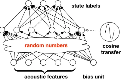
Figure 1: Kernel acoustic model seen as a shallow neural network.
Note thatp(x) can be ignored at inference time because it doesn’t affect the relative scores assigned to different word sequences, andp(y) is simply the prior probability of HMM state
y. The Viterbi algorithm can then be used to determine the most likely word sequence (see Gales and Young (2007) for an overview of using HMMs for speech recognition).
3.3. Kernel Acoustic Models
To train kernel acoustic models, we use random Fourier features and simply plug the random feature vectorz(x) (for an acoustic framex) into a multinomial logistic regression model:
p(y|x) = exp hθy, z(x)i
P
y0exp
θy0, z(x)
. (4)
The label ycan take any value in {1,2, . . . , C}, each corresponding to a context-dependent phonetic state label, and the parameter matrix Θ = [θ1|. . .|θC] is learned. Note that we
also include a bias term in our model by appending a 1 toz(x) in the equation above. The model in Equation (4) can be seen as a shallow neural network, with the following properties: (1) the parameters from the inputs (i.e., acoustic feature vectors) to the hidden units are set randomly, and are not learned; (2) the hidden units use cos(·) as their acti-vation function; (3) the parameters from the hidden units to the output units are learned (can be optimized with convex optimization); and (4) the softmax function is used to nor-malize the outputs of the network. See Figure 1 for a visual representation of this model architecture. Note that although using sinusoidal activation functions has been proposed previously (Goodfellow et al., 2016), their use has remained quite rare in the deep learning context.
3.4. Linear Bottleneck
as a regularization technique, which typically improves the generalization performance of a trained model, as we will show in Section 6.
It is important to note that one can also replace a parameter matrix with a low-rank decomposition after training has completed, for example, using singular value decomposition (Xue et al., 2013). However, in the context of our work it is necessary to impose the low-rank decomposition during training, given GPU memory constraints.
4. Random Feature Selection
In this section, we first motivate and describe our proposed feature selection algorithm. We then introduce a new “sparse Gaussian kernel,” which performs well in conjunction with the feature selection algorithm.
4.1. Proposed Feature Selection Algorithm
Our proposed random feature selection method, shown in Algorithm 1, is iterative. In each iteration, a model is trained on a set of features using a single pass of stochastic gradient descent (SGD) on a subset of the training data. Then, the features whose corresponding rows in the parameter matrix have the smallest `2 norms are discarded and replaced with a new set of random features.
This feature selection method has the following advantages: The overall computational cost is mild, as it requires just T passes of SGD through subsets of the data of size R
(equivalent to T R/N full SGD epochs). In fact, in our experiments, we find it sufficient to use R = O(D). Moreover, the method is able to explore a large number of non-linear features, while maintaining a compact model. If the number of features st selected in
iterationtgrows linearly each iteration (st=Dt/T), then the learning algorithm is exposed toD(T+ 1)/2 random features throughout the feature selection process; this st sequence is the selection schedule we use in all our experiments. We show in Section 6 that the acoustic models trained on the selected features generally outperform models trained on random features.
It is important to note the similarities between this method, and the FOBOS method with `1/`2-regularization (Duchi and Singer, 2009). In the FOBOS method, one solves
the `1/`2-regularized problem in a stochastic fashion by alternating between taking un-regularized stochastic gradient descent (SGD) steps, and then “shrinking” the rows of the parameter matrix; each time the parameters are shrunk, the rows whose`2-norms are below
Algorithm 1 Random feature selection
input Target number of random featuresD, data subset size R,
Integers (s1, . . . , sT−1) such that 0< s1 <· · ·< sT−1 < D, specifying selection schedule.
1: initializeset of selected indices S :=∅. 2: fort= 1,2, . . . , T do
3: for i∈ {1, . . . , D}\S do
4: ωi ∼p(ω).
5: bi∼ U(0,2π). 6: end for
7: if t6=T then
8: Initialize parameter matrix Θ.7
9: Learn weights Θ∈RD×C using a single pass of SGD overRrandomly selected
train-ing examples, ustrain-ing the projection vectors (ω1, . . . ,ωD), and the biases (b1, . . . , bD),
to generate the random Fourier features.
10: S:={i|Θi is amongst thest rows of Θ with highest `2 norm}.8
11: end if
12: end for
13: return The selected projection vectors (ω1, . . . ,ωD), and the selected biases
(b1, . . . , bD).
One disadvantage of this method is that the selection criterion may misrepresent the features’ actual predictive utilities. For instance, the presence of some random feature may increase or decrease the weights for other random features relative to what they would be if that feature were not present. An alternative would be to consider features in isolation, and add features one at a time (as in stagewise regression methods and boosting), but this would be significantly more computationally expensive. For example, it would require
O(D) passes through the data, relative to O(T) passes, which would be prohibitive for largeDvalues. We find empirically that the influence of the additional random features in the selection criterion is tolerable, and it is still possible to select useful features with this method.
4.2. A Sparse Gaussian Kernel
In Section 6 we will show that our proposed feature selection algorithm improves the perfor-mance of the Laplacian kernel models significantly more than the Gaussian kernel models. In this section, we leverage this insight in order to design a new kernel, the “sparse Gaussian kernel,” which we will show also benefits significantly from the feature selection process.
Recall from Table 1 that for the Laplacian kernel, the sampling distribution used for the random Fourier features is the multivariate Cauchy density. Because the Cauchy dis-tribution is fat-tailed, a d-dimensional Cauchy vector will typically contain some entries
7. See Section 6.3 for details on how Θ is initialized.
much larger than the rest. This property of the sampling distribution implies that many of the random features generated via projections with random Cauchy vectors will effectively concentrate on only a few of the input features. We can thus regard such random features as being non-linear combinations of a small number of the original input features. Thus, the proposed feature selection method effectively picks out useful non-linear interactions between small sets of input features.
We can also directly construct sparse non-linear combinations of the input features. Instead of relying on the properties of the Cauchy distribution, we can actually choose a small numberkof coordinatesF ⊆ {1,2, . . . , d}, say, uniformly at random, and then choose the random vector so that it is always zero in positions outside of F. Compared to the random Fourier feature approximation to the Laplacian kernel, the random vectors chosen in this way are truly sparse. From a systems perspective, this sparsity can reduce the memory required for the random projection matrix, and make the random features more efficient to compute (if efficient sparse matrix operations are used).
Note that random Fourier features with such sparse sampling distributions in fact cor-respond to shift-invariant kernels that are rather different from the Laplacian kernel. For instance, if the non-zero entries ofωare drawn i.i.d. fromN(0, σ−2), then the corresponding kernel is
K(x,x0) =
d k
−1 X
F⊆{1,...,d}, |F|=k
exp
−kxF −x
0 Fk22
2σ2
, (5)
wherexF is a vector composed of the elementsxi fori∈F. We call this kernel the “sparse
Gaussian kernel.” Note that this kernel puts equal emphasis on all input feature subsetsF
of sizek. However, the feature selection process may effectively bias the distribution of the feature subsets to concentrate on some small familyF of input feature subsets.
5. New Early Stopping Criteria
A challenge for training acoustic models is that the training criterion (e.g., cross-entropy) does not perfectly correlate with the true objective (TER). To partially address this prob-lem, in this section we present several new metrics which we observe correlate with TER significantly better than cross-entropy does. In Section 6 we then show that we can attain improved TER performance by monitoring these metrics on the heldout set during training to decide when to decay the learning rate and stop training. Note that the reason we use these metrics as proxies for the TER, instead of directly using the TER, is that it is very expensive to compute the TER on the development set.
1. Entropy Regularized Log Loss (ERLL):9 This loss rewards models for being confident (low entropy), by considering a weighted sum of the cross entropy loss (CE) and the average entropy (ENT) of the model on the heldout data. Specifically, for any β∈R, we define the loss as
CE+β·EN T =−1
N N X
i=1 C X
y=1
[I(y=yi) +β·p(y|xi)] logp(y|xi).
This metric encourages models to be more confident, even if it means having a worse cross-entropy loss as a result.
2. Capped Log Loss: For any value ofλ≥0, we define the “capped log loss” as
−1
N N X
i=1
log(p(yi|xi) +λ).
Effectively, this loss ensures that no single example contributes more than−N1 log(λ) to the loss. If λis a small positive number, this loss is very similar to the normal log loss for values of p(yi|xi) close to 1, while affecting the loss dramatically for values
close to 0 (for example, when p(yi|xi)< λ).
3. Top-k Log Loss: For this loss, assume that the heldout examples (xi, yi) are sorted in descending order of theirp(yi|xi) values. Then, for any positive integer k≤N, we
can define the “Top-k Log Loss” as
−1
k k X
i=1
logp(yi|xi).
This metric judges a model based on how well it does on the k heldout examples to which it assigns highest probabilities.
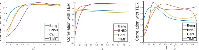
Notice that for β = 0, λ = 0, and k = N, these metrics all simplify to the standard cross-entropy loss. In Figure 2, we show plots of the empirical correlations of these metrics with TER values, as a function of each metric’s “hyperparameters,” based on models we have trained. More specifically, we fully train a large number of kernel and DNN models; we then evaluate the TER performance of these models on the development set, as well as compute the heldout performance of these models in terms of the three metrics described above (for various settings of β,λ, andk). The precise set of models we used are those in Tables 4 and 5. We train models on four data sets: the Cantonese and Bengali data sets for the IARPA Babel program, a 50-hour subset of the broadcast news data set (BN-50), and the TIMIT benchmark task (see Section 6.1 for data set details). We then compute the empirical correlations between the TER values and the different metrics, and plot them as a function of each metric’s hyperparameter. Note that for the top-k log loss, we plot the correlation with TER as a function of the fraction 1− Nk of the heldout data set which is
ignored.
0 0.2 0.4 0.6 0.8 1 1.2 1.4 1.6 1.8 2 β -0.4 -0.2 0 0.2 0.4 0.6 0.8 1
Correlation with TER
Beng BN50 Cant TIMIT
0 0.1 0.2 0.3 0.4 0.5 0.6 0.7 0.8 0.9 1
λ -0.4 -0.2 0 0.2 0.4 0.6 0.8 1
Correlation with TER
Beng BN50 Cant TIMIT
0 0.1 0.2 0.3 0.4 0.5 0.6 0.7 0.8 0.9 1 1− k N -0.4 -0.2 0 0.2 0.4 0.6 0.8 1
Correlation with TER
Beng BN50 Cant TIMIT
Figure 2: Empirical correlations of (left to right) heldout entropy regularized log loss, capped log loss, and top-k log loss with TER on the development set, as a function ofβ,λ, and 1− Nk, respectively.
As can be seen from these plots, for certain ranges of values of the metric hyperparam-eters, the correlation of these metrics with TER is quite high. For example, for β = 1, the correlations between entropy regularized log loss and TER are 0.91, 0.93, 0.90, and 0.95 for Bengali, BN-50, Cantonese, and TIMIT respectively. This is compared to correlations of 0.31,−0.02,−0.23, and −0.21 for the cross-entropy objective.
One conjecture for why these metrics attain higher correlation with ASR performance than heldout cross-entropy is because there is inherent noise in the labels on which the acoustic models are trained. The labels are noisy because they are generated via a forced alignment between the correct transcription and the audio using a GMM/HMM acoustic model, as discussed in Section 6.1. Thus, by not penalizing a model’s mistakes on the incorrect labels as harshly, and instead focusing on the model’s performance on the clean labels, these metrics better capture the quality of the model for the downstream ASR task. Better understanding this phenomenon is an interesting area for future work.
Because of the high correlation between these metrics and ASR performance, we propose to monitor these metrics on the heldout set during training to decide when to decay the learning rate and stop training (details in Section 6.3). In Section 6.4 we present results using this learning rate decay method with the ERLL metric withβ = 1, and show that it leads to improvements in TER for both kernel and DNN models. We note that we could have also used the other metrics for this purpose, but chose to use ERLL with β= 1 since we observed that it attained high correlation values with TER across all four data sets.
6. Experiments
We now present our empirical results comparing the performance of fully-connected DNNs with kernel approximation methods for acoustic modeling, across four data sets. We leverage the three methods we have discussed—feature selection, the new early stopping criterion, and linear bottlenecks—and show that using these three methods the kernel models perform very similarly to the DNNs across the four test sets, attaining token error rates between 0.5% better and 0.1% worse than the DNNs.
hyperparameter choices. We then present our experimental results comparing the perfor-mance of kernel approximation methods to DNNs. Lastly, we discuss the impact of the number of random features on performance, and take a deeper look at the dynamics of the feature selection process.
6.1. Data Sets
We train DNN and kernel acoustic models, as described in Section 3, on four data sets: the IARPA Babel Program Cantonese (IARPA-babel101-v0.4c) and Bengali (IARPA-babel103b-v0.4b) limited language packs, a 50 hour subset of the Broadcast News data set (BN-50) (Kingsbury, 2009; Sainath et al., 2011), and the TIMIT benchmark data set (Garofolo et al., 1993). Each data set is partitioned in four: a training set, a heldout set, a development set, and a test set. We use the heldout set to tune the hyperparameters of our training procedure (e.g., the learning rate). We then run decoding on the development set using IBM’s Attila speech recognition toolkit (Soltau et al., 2010), to select a small subset of models which perform best in terms of TER (the best kernel and DNN model per data set). We tune the acoustic model weight on the development set to optimize the relative contributions of the language model and the acoustic model to the final score assigned to a given word sequence. Finally, we evaluate the TER performance on the test set using the selected group of models (using, for each model, the best acoustic model weight on the development set), to get a fair comparison between the methods we are using. Having a separate development set helps us avoid the risk of over-fitting to the test set.
The Bengali and Cantonese Babel data sets both include training and development sets of approximately 20 hours, and an approximately 5 hour test set. We designate about 10% of the training data as a heldout set. The training, heldout, development, and test sets all contain different speakers. Babel data is challenging because it is two-person conversations between people who know each other well (family and friends) recorded over telephone channels (in most cases with mobile telephones) from speakers in a wide variety of acoustic environments, including moving vehicles and public places. As a result, it contains many natural phenomena such as mispronunciations, disfluencies, laughter, rapid speech, back-ground noise, and channel variability. An additional challenge in Babel is that the only data available for training language models is the acoustic transcripts, which are comparatively small.
For the Broadcast News data set, we use 45 hours of audio for training, and 5 hours as a heldout set. For the development set, we use the EARS Dev-04f data set (as described by Kingsbury, 2009), which consists of approximately three hours of broadcast news from various news shows. We use the DARPA EARS RT-03 English Broadcast News Evaluation Set (Fiscus et al., 2003) as our test set, consisting of 72 five minute conversations.
Data set Train Heldout Dev Test # features # classes Beng. 21 hr (7.7M) 2.8 hr (1.0M) 20 hr (7.1M) 5 hr (1.7M) 360 1000
BN-50 45 hr (16M) 5 hr (1.8M) 2 hr (0.7M) 2.5 hr (0.9M) 360 5000
Cant. 21 hr (7.5M) 2.5 hr (0.9M) 20 hr (7.2M) 5 hr (1.8M) 360 1000 TIMIT 3.2 hr (2.3M) 0.3 hr (0.2M) 0.15 hr (0.1M) 0.15 hr (0.1M) 440 147
Table 2: Data set details. We report the size of each data set partition in terms of the number of hours of speech, and in terms of the number of acoustic frames (in parentheses).
and divisions of the data set as Huang et al. (2014) and Chen et al. (2016), which allows direct comparison of our results with theirs (Table 8).
The acoustic features, representing 25 ms acoustic frames with context, are real-valued dense vectors. A 10 ms shift is used between adjacent frames (except on TIMIT, where a 5 ms shift is used). For the Cantonese, Bengali, and Broadcast News data sets we use a standard 360-dimensional speaker-adapted representation used by IBM (Kingsbury et al., 2013); these feature vectors correspond to the concatenation of nine 40-dimensional vectors corresponding to the four frames before and after the current frame. For the TIMIT experiments, we use 40-dimensional feature space maximum likelihood linear regression (fMLLR) features (Gales, 1998), and concatenate the five neighboring frames in either direction, for a total of eleven frames and 440 features.
The state labels are obtained via forced alignment using a GMM/HMM system. This forced alignment is necessary because there is a mismatch between the ground truth avail-able for training (a word sequence transcribing each utterance) and the actual labels needed for training (precise assignment of HMM states to frames). The Cantonese and Bengali data sets each have 1000 labels, corresponding to quinphone context-dependent HMM states clus-tered using decision trees. For Broadcast News, there are 5000 such states. The TIMIT data set has 147 context-independent labels, corresponding to the beginning, middle, and end of 49 phonemes.
The language models we use are all n-gram language models estimated using modi-fied Kneser-Ney smoothing, with n values of 2, 4, 3, and 3 for Bengali, Broadcast News, Cantonese, and TIMIT, respectively. The TIMIT language model is a phone-level model. The Bengali and Cantonese language models are particularly small (approximately 60,000 bigrams and 136,000 trigrams, respectively), trained using only the provided audio tran-scripts. The Broadcast News model is small as well, containing only 3.3 million 4-grams.
In Table 2 we provide details on all the data sets, as well as on their number of features and classes. All our data sets have millions of training points, significantly exceeding the size of typical machine learning tasks tackled by kernel methods. Additionally, the large number of output classes for our data sets presents a scalability challenge, given that the size of the kernel models scales linearly with the number of output classes (if no bottleneck is used).
6.2. Evaluation Metrics
1. Cross-entropy (CE): Given examples, {(xi, yi), i= 1. . . N}, the cross-entropy is
defined as
−1
N N X
i=1
logp(yi|xi). (6)
2. Average Entropy (ENT): The average entropy of a model is defined as
−1
N N X
i=1 C X
y=1
p(y|xi) logp(y|xi).
If a model has low average entropy, it is generally confident in its predictions.
3. Entropy Regularized Log Loss (ERLL): Defined in Section 5. We use β = 1 unless specified otherwise.
4. Classification Error (ERR): The classification error is defined as
1
N N X
i=1
1
"
yi6= arg max
y∈1,2,...,C
p(y|xi) #
.
5. Token Error Rate (TER): We feed the predictions of the acoustic models, which correspond to probability distributions over the phonetic states, to the rest of the ASR pipeline and calculate the misalignment between the decoder’s outputs and the ground-truth transcriptions. For Bengali and BN-50, we measure the error in terms of the word error rate (WER), for Cantonese we use the character error rate (CER), and for TIMIT we use the phone error rate (PER). We use the term “token error rate” (TER) to refer, for each data set, to its corresponding metric.
6.3. Details of Acoustic Model Training
We train all our kernel models with either the Laplacian, the Gaussian, or the sparse Gaussian (Section 4.2) kernels. These kernel models typically have three hyperparameters: the kernel bandwidth (σ for the Gaussian kernels,λfor the Laplacian kernel; see Table 1), the number of random projections, and the initial learning rate. We try various numbers of random features, ranging from 5000 to 400,000. Using more random features leads to a better approximation of the kernel function, as well as to more powerful models, though there are diminishing returns as the number of features increases. The sparse Gaussian kernel additionally has the hyperparameter k which specifies the sparsity of each random projection vector ωi. For all experiments, we usek= 5.
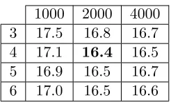
1000 2000 4000
3 17.5 16.8 16.7
4 17.1 16.4 16.5
5 16.9 16.5 16.7
6 17.0 16.5 16.6
Table 3: Effect of depth and width on DNN TER (development set): This table shows TER results for DNNs with 1000, 2000, or 4000 hidden units per layer, and 3-6 layers, on the Broadcast News development set. All of these models were trained using a linear bottleneck for the output parameter matrix, and using ERLL for learning rate decay. The best result is in bold.
the tanh activation function. We vary the number of hidden units per layer (1000, 2000, or 4000). We use this same set of DNN architectures for all our data sets.
For both DNN and kernel models, we use stochastic gradient descent (SGD) as our optimization algorithm for minimizing the training cross-entropy objective. We use mini-batches of size of 250 or 256 samples during training, and we use the heldout set to tune the other hyperparameters. We use the learning rate decay scheme described in (Morgan and Bourlard, 1990; Sainath et al., 2013a,b), which monitors performance on the heldout set to decide when to decay the learning rate. This method divides the learning rate in half at the end of an SGD epoch if the heldout cross-entropy doesn’t improve by at least 1%; additionally, if the heldout cross-entropy gets worse, it reverts the model back to its state at the beginning of the epoch. Instead of using the heldout cross-entropy, in some of our experiments we use the heldout ERLL to decide when to decay the learning rate. We terminate training once we have divided the learning rate 10 times.
As mentioned in Section 3.4, one effective way of reducing the number of parameters in our models is use a linear bottleneck, which is a low-rank factorization of the output parameter matrix (Sainath et al., 2013a). We use bottlenecks of size 1000, 250, 250, and 100 for BN-50, Bengali, Cantonese, and TIMIT, respectively. We train models both with and without this technique; the only exception is that we are unable to train BN-50 kernel models without the bottleneck of size 1000, due to memory constraints on our GPUs.
We initialize our DNN parameters uniformly at random within [−
√ 6 √
din+dout,
√ 6 √
din+dout], as suggested by Glorot and Bengio (2010); here,din and dout refer to the dimensionality of the input and output of a DNN layer, respectively. For our kernel models, we initialize the random projection matrix as discussed in Section 3, and we initialize the parameter matrix Θ as the zero matrix. When using a linear bottleneck to decompose the parameter matrix, we initialize the resulting two matrices randomly, like we do for our DNNs.
and in iteration t, we select st = t·(D/T) = 0.02Dt random features. Thus, the total
computational cost we incur for feature selection is equivalent to approximately seven (or fourteen) epochs of training on the Babel data sets. For the Broadcast News data set, it corresponds to the cost of approximately six full epochs of training (forD≥105).
All our training code is written in MATLAB, leveraging its GPU features, and executed on Amazon EC2 machines.
6.4. Results
In this section, we report the results from our experiments comparing kernel methods to DNNs on ASR tasks. We first discuss the ablation study showing the marginal improvements to the kernel model performance attained by feature selection, the new early stopping criterion, and the linear bottlenecks; we show analogous results for DNNs for the early stopping and linear bottleneck methods. We then compare for each data set the performance of the best kernel and DNN models from these detailed experiments; the most important result from these comparisons, shown in Table 7, is that the kernel models are competitive with the DNNs, attaining TER values between 0.5% better and 0.1% worse than the DNNs across our four test sets.
For our detailed experiments, for both DNN and kernel methods we train models with and without linear bottlenecks, and with and without using ERLL to determine the learning rate decay. For our kernel methods, we additionally train models with and without using feature selection. We run experiments with all three kernels (Laplacian, Gaussian, sparse Gaussian) and we use 100,000 random features on all data sets except for TIMIT, where we are able to use 200,000 random features (because the output dimensionality is lower). As mentioned in the previous section, for our DNN experiments, we train models with four hidden layers,10 using the tanh activation function, and using either 1000, 2000, or 4000 hidden units per layer. We focus on comparing the performance of these methods in terms of TER, but we also report results for other metrics. Unless specified otherwise, all TER results are on the development set, and all cross-entropy, entropy, classification error, and ERLL results are on the heldout set.
In Tables 4 and 5, we show the TER results for our DNN and kernel models, respectively, across all data sets. There are many things to notice about these results. For our DNN models, linear bottlenecks almost always lower TER values, though in a few cases they have no effect on TER. Using ERLL to determine when to decay the learning rate generally helps lower TER values for our DNNs, but in a few cases it actually hurts (Cantonese with 4000 hidden units, and TIMIT with 2000 and 4000). The DNNs with 4000 hidden units typically attain the best results, though on a couple of data sets they are matched or narrowly beaten by the 2000 models.
For our kernel models, we see that incorporating a linear bottleneck brings large drops in TER across the board.11 Performing feature selection generally improves TER as well; we see that it improves TER considerably for the Laplacian kernel, and modestly for the sparse Gaussian kernel. For the Gaussian kernel, it typically helps, though there are several
10. As mentioned in Section 6.3, we find that this is generally the best setting.
instances in which feature selection hurts TER (see Section 6.6 for discussion). Second, we see that using heldout ERLL to determine when to decay the learning rate helps all our kernel models attain lower TER values. Next, we see that without using feature selection, the sparse Gaussian kernel has the best performance across the board. After we include feature selection, it performs very comparably to the Laplacian kernel with feature selection. It is interesting to note that without using feature selection, the Gaussian kernel is generally better than the Laplacian kernel; however, with feature selection, the Laplacian kernel surpasses the Gaussian kernel (see Section 6.6). In general, the kernel function which performed best, across the majority of settings, was the sparse Gaussian kernel.
To further improve the performance of the kernel models, we train models with up to 400k features on Broadcast News, our most challenging data set. Due to the large computational expense of training these models, we only trained a few, and only used the Laplacian and sparse Gaussian kernels, as these attained the best performance after feature selection, in terms of TER. We report results in Table 6. All of these models were trained with a linear bottleneck of size 1000, and using ERLL for learning rate decay. We include results using 100k random features in this table for comparison. As we can observe, our best kernel model on BN-50 now attains a TER of 16.4%, which is equal to the performance of our best DNN model. Furthermore, we continue to see improvements in the performance of our kernel models, even as we increase the number of features beyond 100k; for the Laplacian kernel we get a gain of 0.3% in TER when increasing from 100k to 400k (both with and without feature selection), while for the sparse Gaussian kernel we get gains of 0.2% and 0.4%, with and without feature selection (respectively). To date, these are the largest models we have trained, though it seems likely we could continue getting performance improvements with even larger models.
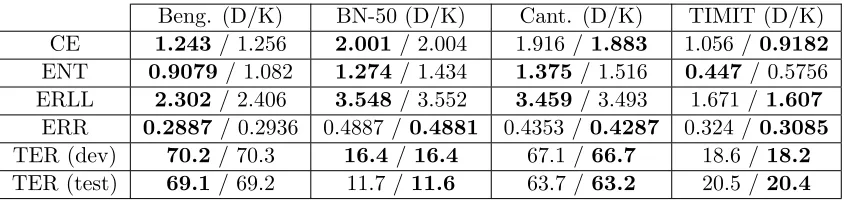
In Table 7, we compare for each data set the performance of the best DNN model with the best kernel model, across six metrics. Importantly, for each metric (except for test set TER), we find the kernel and DNN model which performs best for that specific metric; this is in contrast to picking the kernel and DNN models which are best in terms of TER, and reporting all metrics on these models. For Broadcast News, we consider the kernel models from Table 6 with 200k and 400k random features, along with those in Table 5, in the process of finding the best performing models. In terms of heldout cross-entropy, the kernels outperformed the DNNs on Cantonese and TIMIT, while the DNNs beat the kernels on Bengali and BN-50. With regard to classification error, the kernels beat the DNNs on all data sets except for Bengali. In terms of the average heldout entropy of the models, the DNNs were consistently more confident in their predictions (lower entropy) than the kernels. Significantly, we observe that the best development set TER results for our DNN and kernel models are quite comparable; on Cantonese and TIMIT, the kernel models outperform the DNNs by 0.4% absolute, on Broadcast News the kernels exactly match the DNNs, while on Bengali the DNNs do better by 0.1%.
We now discuss the results on the test sets. First of all, to avoid overfitting to the test sets, for each data set we only performed test set evaluations for the DNN and kernel models which performed best in terms of the development set TER. The final row of Table 7 thus contains all the test results we collected.12 As one can see, the relative test performance 12. The only exception is on the Broadcast News data set. Prior to training the best performing 400k model,
1000 2000 4000
NT B R BR NT B R BR NT B R BR
Beng. 72.3 71.6 71.7 70.9 71.5 71.1 70.7 70.3 71.1 70.6 70.5 70.2
BN-50 18.0 17.3 17.8 17.1 17.4 16.7 17.1 16.4 16.8 16.7 16.7 16.5
Cant. 68.4 68.1 67.9 67.5 67.7 67.7 67.2 67.1 67.7 67.1 67.2 67.2
TIMIT 19.5 19.3 19.4 19.2 19.0 18.9 19.2 19.2 18.6 18.6 18.7 18.9
Table 4: DNN TER Results (development set): This table shows TER results for 4-hidden layer DNNs with 1000, 2000, or 4000 hidden units per layer. ‘NT’ specifies that no “tricks” were used during training (no bottleneck, did not use ERLL for learning rate decay). A ‘B’ specifies that a linear bottleneck was used; an ‘R’ specifies that ERLL was used for learning rate decay (so ‘BR’ means both were used). The best result for each data set is in bold.
Laplacian Gaussian Sparse Gaussian
NT B R BR NT B R BR NT B R BR
Beng. 74.5 72.1 74.5 71.4 72.6 72.0 72.6 71.8 73.0 71.5 73.0 70.9
+FS 72.9 71.1 72.8 70.4 74.1 71.4 74.2 70.3 72.9 71.2 72.8 70.7
BN-50 N/A 17.9 N/A 17.7 N/A 17.3 N/A 17.1 N/A 17.3 N/A 17.0
+FS N/A 17.1 N/A 16.7 N/A 17.5 N/A 17.0 N/A 17.1 N/A 16.7
Cant. 69.9 68.2 69.2 67.4 70.2 67.6 70.0 67.1 68.6 67.5 68.1 67.1
+FS 68.4 67.5 68.5 66.7 69.9 67.7 69.8 66.9 68.6 67.4 68.5 66.8
TIMIT 20.6 19.2 20.4 18.9 19.8 18.9 19.6 18.6 19.9 18.8 19.6 18.4
+FS 19.5 18.6 19.3 18.4 19.5 18.6 19.4 18.4 19.3 18.4 19.1 18.2
Table 5: Kernel TER Results (development set): This table shows TER results for our ker-nel experiments using either the Laplacian, Gaussian, or Sparse Gaussian kerker-nels, with 100k random features (except for TIMIT, which uses 200k features). ‘NT’ specifies that no “tricks” were used during training (no bottleneck, did not use ERLL for learning rate decay). A ‘B’ specifies that a linear bottleneck was used; an ‘R’ specifies that ERLL was used for the learning rate decay (so ‘BR’ means both were used). ‘+FS’ specifies that feature selection was used. The best result for each row is in bold.
100k 200k 400k
Laplacian 17.7 17.7 17.4
+FS 16.7 16.4 16.4
Sparse Gaussian 17.0 16.8 16.6
+FS 16.7 16.6 16.5
Beng. (D/K) BN-50 (D/K) Cant. (D/K) TIMIT (D/K)
CE 1.243/ 1.256 2.001/ 2.004 1.916 /1.883 1.056 /0.9182
ENT 0.9079 / 1.082 1.274/ 1.434 1.375/ 1.516 0.447/ 0.5756
ERLL 2.302/ 2.406 3.548/ 3.552 3.459/ 3.493 1.671 /1.607
ERR 0.2887 / 0.2936 0.4887 / 0.4881 0.4353 /0.4287 0.324 /0.3085
TER (dev) 70.2 / 70.3 16.4 /16.4 67.1 /66.7 18.6 /18.2
TER (test) 69.1 / 69.2 11.7 /11.6 63.7 /63.2 20.5 /20.4
Table 7: Table comparing the Best DNN (‘D’) and kernel (‘K’) results, across four data sets and six metrics. The first four metrics are on the heldout set, the fifth is on the development set, and the last metric is reported on the test set. For BN50, the large models from Table 6 are included in the set of models from which the best performing model is picked (for each metric). See Section 6.2 for metric definitions.
Test TER (DNN) Test TER (Kernel)
Huang et al. (2014) 20.5 21.3
Chen et al. (2016) N/A 20.9
This work 20.5 20.4
Table 8: Table comparing the Best DNN and kernel results from this work to those from Huang et al. (2014) and Chen et al. (2016), on the TIMIT test set.
of the DNN and kernel models is quite similar to the development set results; the DNNs perform better by 0.5% on Cantonese, 0.1% on TIMIT and Broadcast News, and perform worse by 0.1% on Bengali. For direct comparison on the TIMIT data set, we include in Table 8 the test results for the best DNN and kernel models from Huang et al. (2014) and Chen et al. (2016). As mentioned in Section 6.1, we use the same features, labels, data set partitions (train/heldout/dev/test), and decoding script as these papers, and thus our results are directly comparable. We achieve a 0.9% absolute improvement in TER with our kernel model relative to Huang et al. (2014), and 0.5% improvement relative to Chen et al. (2016); furthermore, our best DNN matches the performance of the best performing DNN from Huang et al. (2014). We believe the most significant of all these results is that the kernels (narrowly) beat the DNNs on Broadcast News, our largest and most challenging data set, and one which has been used extensively in large scale speech recognition research. In Appendix A, we include more detailed tables comparing the various models we trained across all the metrics from Section 6.2.
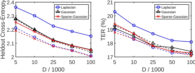
6.5. Importance of the Number of Random Features
We will now illustrate the importance of the number of random features D on model performance. For this purpose, we trained kernel models on the BN-50 data set using
dramat-5 10 25 50 100
D / 1000
2 2.1 2.2 2.3 2.4
Heldout Cross-Entropy
Laplacian Gaussian Sparse-Gaussian
5 10 25 50 100
D / 1000
1718 19 20 21
TER (%)
Laplacian Gaussian Sparse-Gaussian
Figure 3: Heldout cross-entropy and development set TER performance of kernel acoustic models on BN-50, as a function of the number of random features D. Dashed lines mean feature selection was performed, while solid lines mean it was not.
ically improves the performance of the learned model, both in terms of cross-entropy and TER; there are diminishing returns, however, with small improvements in TER when in-creasingDfrom 50,000 to 100,000. Interestingly, we can also observe in these plots that the benefits from feature selection (gap between the dashed and solid lines) are large for the Laplacian kernel, modest for the sparse Gaussian kernel, and insignificant for the Gaussian kernel. We provide insight into why these trends occur in the following section.
6.6. Dynamics of Random Feature Selection
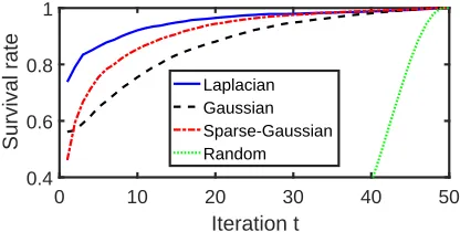
We now explore the feature selection dynamics. We first show that features selected in early iterations are likely to be selected in all subsequent iterations, demonstrating that the selection criterion is consistent. Second, we show that the feature selection process can be seen as way of learning to upweight important input features. This effect is pronounced for the Laplacian and sparse Gaussian kernels, but not for the Gaussian kernel, helping to explain why the former methods benefit from feature selection more than the latter.
In Figure 4, we plot the fraction of the st features selected in iterationt that remain in the model after allT iterations (“survival rate”). We show results for kernel models trained on the Cantonese data set, without using linear bottlenecks, and using heldout cross-entropy for learning rate decay. In nearly all iterations and for all kernels, over half of the selected features survive to the final model. For instance, over 90% of the Laplacian kernel features selected at iteration 10 survive the remaining 40 rounds of selection. For comparison, we plot the expected survival rate if at each iteration the features were chosen uniformly at random; for st = Dt/T, the expected survival rate for features selected at iteration t is
T!/(t!·TT−t), which is exponentially small in T when t≤ βT for any fixed β < 1.13 For example, at t = 10 the expected survival rate is approximately 9×10⁻¹¹ with T = 50. Thus, our selection criterion is orders of magnitude more consistent than random selection.
0 10 20 30 40 50
Iteration t
0.4 0.6 0.8 1
Survival rate
Laplacian Gaussian Sparse-Gaussian Random
Figure 4: Fraction of the st features selected in iteration t that are in the final model
(survival rate) for kernel models trained on the Cantonese data set.
0 100 200 300
Input feature number 1
3 5 7
Relative weight
Laplacian Gaussian Sparse-Gaussian
Figure 5: The relative weight of each input feature in the projection matrix Ω after feature selection completes, for kernel models trained on the Cantonese data set.
Finally, we consider how the feature selection process can be seen as a way of learning to assign more weight to the more important input features. Consider the final matrix of random vectors Ω := [ω1, . . . ,ωD]∈Rd×D after feature selection, for the Cantonese models
from Figure 4. A coarse measure of how much influence an input feature i∈ {1,2, . . . , d} has in the final feature map is the relative “weight” of the i-th row of Ω. In Figure 5, we plot PDj=1|Ωi,j|/Z for each input feature i∈ {1,2, . . . , d}, where Z = 1dPi,j|Ωi,j| is a
normalization term.14 There is a strong periodic effect as a function of the input feature number. An examination of the feature pipeline from Kingsbury et al. (2013) reveals that this is because these features vectors are the concatenation of nine 40-dimensional acoustic feature vectors, where each set of 40 features is ordered by a measure of discriminative quality (via linear discriminant analysis). Thus, it is expected that the features with low (i−1) mod 40 value may be more useful than the others; indeed, this is evident in the plot. Note that this effect exists, but is extremely weak, for the Gaussian kernel. We believe this is because Gaussian random vectors in Rd are likely to have all their entries be bounded in
magnitude byO(plog(d)). This observation helps explain why feature selection significantly improves the Laplacian and sparse Gaussian models, but not the Gaussian models.
7. Conclusion
In this paper, we explore the performance of kernel methods on large-scale ASR tasks, lever-aging the kernel approximation technique of Rahimi and Recht (2007). We propose two new methods (feature selection, new early stopping criteria) which lead to large improvements in the performance of kernel acoustic models. We further show that using a linear bottleneck (Sainath et al., 2013a) to decompose the parameter matrices of these kernel models leads to significant improvements in performance as well. We validate these findings on four data sets, including the Broadcast News and TIMIT benchmark tasks. Using all these methods together, the kernel methods attain comparable speech recognition performance to DNNs across the four test sets; on Cantonese, TIMIT, and Broadcast News, the kernel models outperform the DNNs by 0.5%, 0.1%, and 0.1% TER absolute, respectively, whereas on Bengali, the DNN does better by 0.1% TER.
For future work, we are interested in continuing to test the limits of kernel methods on challenging empirical tasks. For example, can kernel methods be adapted to compete with convolutional and recurrent neural networks?
Acknowledgments
This research is supported by the Intelligence Advanced Research Projects Activity (IARPA) via Department of Defense U.S. Army Research Laboratory (DoD / ARL) contract num-ber W911NF-12-C-0012. The U.S. Government is authorized to reproduce and distribute reprints for Governmental purposes notwithstanding any copyright annotation thereon. Dis-claimer: The views and conclusions contained herein are those of the authors and should not be interpreted as necessarily representing the official policies or endorsements, either expressed or implied, of IARPA, DoD/ARL, or the U.S. Government.
Appendix A. Detailed Empirical Results
In this appendix, we include tables comparing the models we trained in terms of four different metrics (CE, ENT, ERR, and ERLL). The notation is the same as in Tables 4 and 5. For both DNN and kernel models, ‘NT’ specifies that no “tricks” were used during training (no bottleneck, did not use ERLL for learning rate decay). A ‘B’ specifies that a linear bottleneck was used for the output parameter matrix, while an ‘R’ specifies that ERLL was used for learning rate decay (so ‘BR’ means both were used). For kernel models, ‘+FS’ specifies that feature selection was performed for the corresponding row. The best result for each metric and data set is in bold.
Some important things to take note of in these tables:
• The linear bottleneck typically causes large drops in the average entropy of kernel mod-els, while not having as strong or consistent an effect on cross-entropy. For DNNs, the bottleneck typically causes increases in cross-entropy, and relatively modest decreases in entropy.
• Using ERLL to determine learning rate decay typically causes increases in cross-entropy, and decreases in cross-entropy, with the decrease in entropy typically being larger than the increase in cross-entropy. As a result, the ERLL is typically lower for models that use this method (with the exception of TIMIT DNN models).
• Feature selection typically results in large drops in cross-entropy, especially for Lapla-cian and sparse Gaussian kernels, while its effect on entropy is quite small. It thus helps lower heldout ERLL across the board, as well as TER in the vast majority of cases.
Laplacian Gaussian Sparse Gaussian
NT B R BR NT B R BR NT B R BR
Beng. 1.34 1.32 1.35 1.39 1.35 1.33 1.36 1.34 1.31 1.29 1.34 1.33
+FS 1.28 1.26 1.29 1.27 1.35 1.31 1.36 1.35 1.28 1.26 1.31 1.27
BN-50 N/A 2.15 N/A 2.43 N/A 2.05 N/A 2.16 N/A 2.05 N/A 2.19
+FS N/A 2.01 N/A 2.07 N/A 2.04 N/A 2.13 N/A 2.00 N/A 2.06
Cant. 1.93 1.95 1.95 2.04 1.99 1.98 2.00 2.04 1.93 1.94 1.95 2.00
+FS 1.88 1.90 1.89 1.95 1.97 1.97 1.98 2.03 1.90 1.91 1.91 1.96
TIMIT 0.97 0.99 0.97 1.07 0.94 0.96 0.94 1.02 0.94 0.95 0.94 1.03
+FS 0.92 0.95 0.92 1.03 0.93 0.96 0.93 1.02 0.92 0.96 0.92 1.03
1000 2000 4000
NT B R BR NT B R BR NT B R BR
Beng. 1.25 1.26 1.24 1.27 1.24 1.26 1.26 1.32 1.24 1.25 1.30 1.39
BN-50 2.05 2.05 2.04 2.08 2.01 2.04 2.05 2.22 2.00 2.03 2.09 2.27
Cant. 1.92 1.96 1.92 1.98 1.93 1.94 1.97 2.06 1.92 1.97 2.03 2.10
TIMIT 1.06 1.08 1.20 1.28 1.08 1.09 1.25 1.31 1.10 1.11 1.25 1.33
Table 10: DNN: Metric CE
Laplacian Gaussian Sparse Gaussian
NT B R BR NT B R BR NT B R BR
Beng. 1.43 1.23 1.41 1.08 1.36 1.31 1.35 1.28 1.35 1.23 1.30 1.10
+FS 1.32 1.21 1.28 1.14 1.44 1.27 1.45 1.13 1.32 1.22 1.26 1.14
BN-50 N/A 1.89 N/A 1.46 N/A 1.83 N/A 1.53 N/A 1.81 N/A 1.48
+FS N/A 1.81 N/A 1.56 N/A 1.84 N/A 1.55 N/A 1.80 N/A 1.57
Cant. 1.84 1.67 1.76 1.52 1.94 1.73 1.91 1.58 1.77 1.69 1.70 1.55
+FS 1.75 1.66 1.73 1.54 1.91 1.72 1.87 1.57 1.75 1.68 1.72 1.54
TIMIT 0.95 0.72 0.91 0.61 0.88 0.73 0.86 0.62 0.89 0.76 0.85 0.61
+FS 0.86 0.70 0.82 0.58 0.86 0.70 0.83 0.61 0.84 0.69 0.82 0.58
Table 11: Kernel: Metric ENT
1000 2000 4000
NT B R BR NT B R BR NT B R BR
Beng. 1.23 1.17 1.18 1.09 1.18 1.13 1.09 0.99 1.14 1.11 1.02 0.91
BN-50 1.95 1.77 1.90 1.68 1.76 1.68 1.65 1.40 1.65 1.60 1.48 1.27
Cant. 1.71 1.67 1.67 1.57 1.66 1.64 1.55 1.42 1.63 1.55 1.43 1.38
TIMIT 0.72 0.70 0.58 0.53 0.63 0.63 0.50 0.48 0.57 0.57 0.48 0.45
Table 12: DNN: Metric ENT
Laplacian Gaussian Sparse Gaussian
NT B R BR NT B R BR NT B R BR
Beng. 2.77 2.55 2.76 2.47 2.71 2.65 2.71 2.62 2.67 2.52 2.64 2.44
+FS 2.60 2.47 2.57 2.41 2.79 2.58 2.80 2.48 2.60 2.48 2.57 2.41
BN-50 N/A 4.04 N/A 3.88 N/A 3.88 N/A 3.69 N/A 3.86 N/A 3.67
+FS N/A 3.82 N/A 3.63 N/A 3.88 N/A 3.67 N/A 3.80 N/A 3.62
Cant. 3.77 3.62 3.71 3.56 3.94 3.71 3.91 3.62 3.71 3.63 3.65 3.54
+FS 3.63 3.56 3.63 3.49 3.88 3.69 3.86 3.60 3.64 3.58 3.63 3.50
TIMIT 1.92 1.71 1.87 1.68 1.82 1.70 1.80 1.65 1.83 1.71 1.79 1.64
+FS 1.78 1.65 1.74 1.61 1.79 1.67 1.76 1.64 1.76 1.64 1.74 1.61
1000 2000 4000
NT B R BR NT B R BR NT B R BR
Beng. 2.48 2.43 2.43 2.37 2.42 2.39 2.35 2.31 2.39 2.37 2.32 2.30
BN-50 3.99 3.82 3.94 3.76 3.77 3.72 3.70 3.63 3.65 3.63 3.58 3.55
Cant. 3.63 3.63 3.58 3.56 3.59 3.58 3.51 3.48 3.55 3.52 3.46 3.47
TIMIT 1.77 1.77 1.77 1.81 1.71 1.72 1.76 1.79 1.67 1.68 1.73 1.78
Table 14: DNN: Metric ERLL
Laplacian Gaussian Sparse Gaussian
NT B R BR NT B R BR NT B R BR
Beng. 0.30 0.30 0.31 0.31 0.31 0.31 0.31 0.31 0.30 0.30 0.30 0.30
+FS 0.29 0.29 0.30 0.29 0.31 0.31 0.31 0.31 0.30 0.29 0.30 0.30
BN-50 N/A 0.52 N/A 0.54 N/A 0.50 N/A 0.51 N/A 0.50 N/A 0.51
+FS N/A 0.49 N/A 0.50 N/A 0.50 N/A 0.50 N/A 0.49 N/A 0.49
Cant. 0.43 0.44 0.44 0.44 0.45 0.45 0.45 0.45 0.43 0.44 0.44 0.44
+FS 0.43 0.43 0.43 0.44 0.44 0.44 0.44 0.45 0.43 0.44 0.43 0.44
TIMIT 0.32 0.32 0.32 0.33 0.31 0.32 0.31 0.32 0.31 0.31 0.31 0.32
+FS 0.31 0.31 0.31 0.31 0.31 0.31 0.31 0.32 0.31 0.31 0.31 0.31
Table 15: Kernel: Metric ERR
1000 2000 4000
NT B R BR NT B R BR NT B R BR
Beng. 0.29 0.29 0.29 0.29 0.29 0.29 0.29 0.30 0.29 0.29 0.29 0.30
BN-50 0.50 0.50 0.50 0.50 0.49 0.50 0.50 0.51 0.49 0.49 0.50 0.51
Cant. 0.44 0.44 0.44 0.44 0.44 0.44 0.44 0.44 0.44 0.44 0.44 0.44
TIMIT 0.33 0.33 0.34 0.34 0.33 0.33 0.34 0.34 0.33 0.32 0.33 0.33