Kernel Density Estimation for Dynamical Systems
Hanyuan Hang [email protected]
Institute of Statistics and Big Data Renmin University of China 100872 Beijing, China
Ingo Steinwart [email protected]
Institute for Stochastics and Applications University of Stuttgart
70569 Stuttgart, Germany
Yunlong Feng [email protected]
Department of Mathematics and Statistics State University of New York
The University at Albany Albany, New York 12222, USA
Johan A.K. Suykens [email protected]
Department of Electrical Engineering, ESAT-STADIUS, KU Leuven Kasteelpark Arenberg 10, Leuven, B-3001, Belgium
Editor:John Shawe-Taylor
Abstract
We study the density estimation problem with observations generated by certain dynamical systems that admit a unique underlying invariant Lebesgue density. Observations drawn from dynamical systems are not independent and moreover, usual mixing concepts may not be appropriate for measuring the dependence among these observations. By employing the C-mixing concept to measure the dependence, we conduct statistical analysis on the consistency and convergence of the kernel density estimator. Our main results are as follows: First, we show that with properly chosen bandwidth, the kernel density estimator is universally consistent under L1-norm; Second, we establish convergence rates for the
estimator with respect to several classes of dynamical systems under L1-norm. In the
analysis, the density function f is only assumed to be H¨older continuous or pointwise H¨older controllable which is a weak assumption in the literature of nonparametric density estimation and also more realistic in the dynamical system context. Last but not least, we prove that the same convergence rates of the estimator underL∞-norm andL1-norm
can be achieved when the density function is H¨older continuous, compactly supported, and bounded. The bandwidth selection problem of the kernel density estimator for dynamical system is also discussed in our study via numerical simulations.
Keywords: Kernel density estimation, dynamical system, dependent observations, C -mixing process, universal consistency, convergence rates, covering number, learning theory
c
1. Introduction
Dynamical systems are now ubiquitous and are vital in modeling complex systems, espe-cially when they admit recurrence relations. Statistical inference for dynamical systems has drawn continuous attention across various fields, the topics of which include param-eter estimation, invariant measure estimation, forecasting, noise detection, among others. For instance, in the statistics and machine learning community, the statistical inference for certain dynamical systems have been recently studied in Suykens et al. (1995); Suykens and Vandewalle (2000); Suykens et al. (2002); Zoeter and Heskes (2005); Anghel and Stein-wart (2007); SteinStein-wart and Anghel (2009); Deisenroth and Mohamed (2012); McGoff et al. (2015a); Hang and Steinwart (2017), just to name a few. We refer the reader to a recent survey in McGoff et al. (2015b) for a general depiction of this topic. The purpose of this study is to investigate the density estimation problem for dynamical systems via a classical nonparametric approach, i.e., kernel density estimation.
The commonly considered density estimation problem can be stated as follows. Let x1, x2, . . . , xn be observations drawn independently from an unknown distribution P on Rd
with the density f. Density estimation is concerned with the estimation of the underlying densityf. Accurate estimation of the density is important for many machine learning tasks such as regression, classification, and clustering problems and also plays an important role in many real-world applications. Nonparametric density estimators are popular since weaker assumptions are applied to the underlying probability distribution. Typical nonparametric density estimators include the histogram and kernel density estimator. In this study, we are interested in the latter one, namely, kernel density estimator, which is also termed as
Parzen-Rosenblatt estimator (Parzen, 1962; Rosenblatt, 1956) and takes the following form
fn(x) =
1
nhd n
X
i=1 K
x−xi h
. (1)
Here, h := hn > 0 is a bandwidth parameter and K is a smoothing kernel. In the
lit-erature, point-wise and uniform consistency and convergence rates of the estimator fn to
the unknown truth density f under various distance measurements, e.g., L1, L2, and L∞,
have been established by resorting to the regularity assumptions on the smoothing kernel
K, the density f, and the decay of the bandwidth sequence {hn}. Besides the theoretical
concerns on the consistency and convergence rates, another practical issue one usually needs to address is the choice of the bandwidth parameterhn, which is also called thesmoothing parameter. It plays a crucial role in the bias-variance trade-off in kernel density estimation. In the literature, approaches to choosing the smoothing parameter include least-squares cross-validation (Bowman, 1984; Rudemo, 1982), biased cross-validation (Scott and Terrell, 1987), plug-in method (Park and Marron, 1990; Sheather and Jones, 1991), the double kernel method (Devroye, 1989), and also the method based on a discrepancy principle (Eg-germont and LaRiccia, 2001). We refer the reader to Jones et al. (1996a) for a general overview and to Wand and Jones (1994); Cao et al. (1994); Jones et al. (1996b); Devroye (1997) for more detailed reviews.
given data can be very much restrictive in real-world applications. Having realized this, researchers turn to weaken this i.i.d assumption by assuming that the observations are weakly dependent under various notions of weakly dependence which include α-mixing,
β-mixing, and φ-mixing (Bradley, 2005). There has been a flurry of work to attack this problem with theoretical and practical concerns, see e.g., Gy¨orfi (1981); Masry (1983, 1986); Robinson (1983); Masry and Gy¨orfi (1987); Tran (1989b); Gy¨orfi and Masry (1990); Tran (1989a); Hart and Vieu (1990); Yu (1993) and Hall et al. (1995), under the above notions of dependence. These studies were conducted under various notions of sample dependence. In fact, as Gy¨orfi and Lugosi (1992) pointed out, for samples that are ergodic, kernel density estimation is not universally consistent under the usual conditions. A counter example was devised there showing the existence of an ergodic sequence of uniformly distributed random variables based on which the kernel density estimation almost surely does not tend to zero in the L1 sense. On the other hand, the assumed correlation among the observations
complicates the kernel density estimation problem from a technical as well as practical view and also brings inherent barriers. This is because, more frequently, the analysis on the consistency and convergence rates of the kernel density estimator (1) is proceeded by decomposing the error term into bias and variance terms, which correspond to data-free and data-dependent error terms, respectively. The data-free error term can be tackled by using techniques from the approximation theory while the data-dependent error term is usually dealt with by exploiting arguments from the empirical process theory such as concentration inequalities. As a result, due to the existence of dependence among observations and various notions of the dependence measurement, the techniques, and results concerning the data-dependent error term are in general not universally applicable. On the other hand, it has been also pointed out that the bandwidth selection in kernel density estimation under dependence also departures from the independent case, see e.g., Hart and Vieu (1990); Hall et al. (1995).
In fact, when the observations x1, x2, . . . , xn ∈ Rd are generated by certain ergodic
measure-preserving dynamical systems, the problem of kernel density estimation can be even more involved. To explain, let us consider a discrete-time ergodic measure-preserving dynamical system described by the sequence (Tn)n≥1 of iterates of an unknown map T :
Ω → Ω with Ω⊂ Rd and a unique invariant measure P which possesses a density f with
respect to the Lebesgue measure (rigorous definitions will be given in the sequel). That is, we have
xi =Ti(x0), i= 1,2, . . . , n, (2)
where x0 is the initial state. It is noticed that in this case the usual mixing concepts are
not general enough to characterize the dependence among observations generated by (2) (Maume-Deschamps, 2006; Steinwart and Anghel, 2009; Hang and Steinwart, 2017). On the other hand, existing theoretical studies on the consistency or convergence rates of the kernel density estimator for i.i.d. observations frequently assume that the density function
of bounded variation. Typical examples are the Gauss map in Example 3 and the β-maps in Example 1 (see Subsection 2.2).
In this study, the kernel density estimation problem with observations generated by dynamical systems (2) is approached by making use of a more general concept for measuring the dependence of observations, namely, the so-called C-mixing process (refer to Section 2 for the definition). Proposed in Maume-Deschamps (2006) and recently investigated in Hang and Steinwart (2017), theC-mixing concept is shown to be more general and powerful in measuring dependence among observations generated by dynamical systems and can accommodate a large class of dynamical systems. There, a Bernstein-type exponential inequality for C-mixing processes was established and its applications to some learning schemes were explored.
Our main purpose in this paper is to conduct some theoretical analysis and practical im-plementations on the kernel density estimator for dynamical systems. The primary concern is the consistency and convergence rates of the kernel density estimator (1) with observations generated by dynamical systems (2). The consistency and convergence analysis is conducted underL1-norm, andL∞-norm, respectively. We show that under mild assumptions on the
smoothing kernel, with properly chosen bandwidth, the estimator is universally consistent underL1-norm. When the probability distributionP possesses a polynomial or exponential
decay outside of a radius-r ball in its support, under the H¨older continuity assumptions on the kernel function and the density, we obtain almost optimal convergence rates under
L1-norm. Moreover, when the probability distributionP is compactly supported, which is
a frequently encountered setting in the dynamical system context, we prove that stronger convergence results of the estimator can be developed, i.e., convergence results under L ∞-norm which are shown to be of the same order with itsL1-norm convergence rates. Finally,
with regard to the practical implementation of the estimator, we also discuss the bandwidth selection problem by performing numerical comparisons among several typical existing selec-tors that include least squares cross-validation and its variants for dependent observations, and the double kernel method. We show that the double kernel bandwidth selector pro-posed in Devroye (1989) can in general work well. Moreover, according to our numerical experiments, we find that bandwidth selection for kernel density estimator of dynamical systems is usually ad-hoc in the sense that its performance may depend on the considered dynamical system.
2. Preliminaries
2.1 Notations
Throughout this paper,λdis denoted as the Lebesgue measure on
Rdandk·kis an arbitrary
norm on Rd. We denoteBr as the centered ball of Rdwith radius r, that is,
Br :={x= (x1, . . . , xd)∈Rd:kxk ≤r}.
Recall that for 1≤ p <∞, the `dp-norm is defined as kxk`d p := (x
p
1 +· · ·+x p
d)1/p, and the `d∞-norm is defined as kxk`d
∞ := maxi=1,...,d|xi|. Let (Ω,A, µ) be a probability space. We denote Lp(µ) as the space of (equivalence classes of) measurable functions g: Ω→Rwith
finite Lp-norm kgkp. Then Lp(µ) together with kgkp forms a Banach space. Moreover, if
A0 ⊂ A is a sub-σ-algebra, then L
p(A0, µ) denotes the space of all A0-measurable functions g∈Lp(µ). Finally, for a Banach space E, we writeBE for its closed unit ball.
In what follows, the notationan.bnmeans that there exists a positive constant csuch
that an ≤ c bn, for all n ∈ N. With a slight abuse of notation, in this paper, c, c0 and C
are used interchangeably for positive constants while their values may vary across different lemmas, propositions, theorems, and corollaries.
2.2 Dynamical Systems and C-mixing Processes
In this subsection, we first introduce the dynamical systems of interest, namely, ergodic measure-preserving dynamical systems. Mathematically, anergodic measure-preserving dy-namical system is a system (Ω,A, µ, T) with a mapping T : Ω → Ω that is measure-preserving, i.e., µ(A) = µ(T−1A) for all A ∈ A, and ergodic, i.e., T−1A = A implies
µ(A) = 0 or 1. In this study, we are confined to the dynamical systems in which Ω is a subset of Rd, µ is a probability measure that is absolutely continuous with respect to the
Lebesgue measureλdand admits a unique invariant Lebesgue densityf. In order to include a larger variety of density functions that commonly appear in dynamical systems, we intro-duce a new measurement of continuity that is a generalization of the α-H¨older continuity, which is defined as follows:
Definition 1 (Pointwise α-H¨older Controllable) A density function f :Rd → [0,∞) is called pointwise α-H¨older controllable, if for λd-almost allx∈Rd there exists a constant c(x)≥0 and a radius r(x)>0 such that for all x0∈Rd withkx0k< r(x) we have
|f(x+x0)−f(x)| ≤c(x)kx0kα.
Moreover, f is called uniformly pointwiseα-H¨older controllable, if
r0 := ess inf
x∈Ωr(x)>0.
Note that the an α-H¨older continuous function can be recognized as a special case of theα-H¨older controllable functions withc(x) andr(x) being some universal constantc >0 and r >0.
In our study, it is assumed that the observations x1, x2,· · ·, xn are generated by the
Example 1 (β-Map) For β >1, the β-map is defined as T(x) =βx mod 1, x∈(0,1),
with a unique invariant Lebesgue density given by
f(x) =cβ
X
i≥0
β−(i+1)1[0,Ti(1)](x),
where cβ is a constant chosen such that f has integral 1.
Example 2 (Logistic Map) The Logistic map defined by T(x) = 4x(1−x), x∈(0,1)
admits the unique invariant Lebesgue density
f(x) = 1
πpx(1−x) ·1(0,1)(x), x∈R.
Moreover, for all α∈(0,1/2), the density f isα-H¨older controllable with
c(x) :=
0 if x <0
x−1/2−α if 0< x <1/4
4 if 1/4≤x≤3/4
(1−x)−1/2−α if 3/4≤x <1 0 if x >1.
and
r(x) :=
−x if x <0
x/2 if 0< x <1/4 1/4 if 1/4≤x≤3/4
1−x/2 if 3/4≤x <1
x−1 if x >1.
(3)
Example 3 (Gauss Map) The Gauss map is defined by T(x) = 1
x mod 1, x∈(0,1),
with a unique invariant Lebesgue density
f(x) = 1 log 2 ·
1
1 +x ·1[0,1](x), x∈R.
We now introduce the notion for measuring the dependence among observations from dynamical systems, namely, C-mixing process. To this end, let us assume that (X,B) is a measurable space with X ⊂Rd. Let X := (X
n)n≥1 be an X-valued stochastic process on
(Ω,A, µ), and for 1≤i ≤j ≤ ∞, denote by Aji the σ-algebra generated by (Xi, . . . , Xj).
Let Γ : Ω →X be a measurable map. µΓ is denoted as theΓ-image measure ofµ, which
is defined as µΓ(B) :=µ(Γ−1(B)), B ⊂X measurable. The processX is calledstationary
ifµ(Xi1+j,...,Xin+j)=µ(Xi1,...,Xin) for all n, j, i1, . . . , in≥1. DenoteP :=µX1. Moreover, for
ψ, ϕ∈L1(µ) satisfyingψϕ∈L1(µ), we denote the correlation of ψand ϕby
cor(ψ, ϕ) :=
Z
Ω
ψ ϕdµ− Z
Ω ψdµ·
Z
Ω ϕdµ .
It is shown that several dependency coefficients for X can be expressed in terms of such correlations for restricted sets of functions ψ and ϕ. In order to introduce the notion, we also need to define a new norm which introduces restrictions on ψ and ϕ considered here. Throughout this paper, C(X) is denoted as a subspace of bounded measurable functions
g : X → R and that we have a semi-norm ||| · ||| on C(X). For g ∈ C(X), we define the
C-normk · kC by
kgkC :=kgk∞+|||g|||. (4)
Additionally, we need to introduce the following restrictions on the semi-norm ||| · |||.
Assumption A We assume that the following two restrictions on the semi-norm ||| · |||
hold:
(i) |||g|||= 0 for all constant functions g∈ C(X);
(ii) |||eg||| ≤ eg
∞|||g|||, g∈ C(X).
Note that the first constraint on the semi-norm in Assumption A implies its shift invariance onRwhile the inequality constraint can be viewed as an abstractchain ruleif one views the
semi-norm as a norm describing aspects of the smoothness ofg. In fact, it is easy to show that the following function classes, which are probably also the most frequently considered in the dynamical system context, satisfy Condition (i) in Assumption A. Moreover, they also satisfy Condition (ii) in Assumption A, as shown in Hang and Steinwart (2017):
• L∞(X): The class of bounded functions on X;
• BV(X): The class of bounded variation functions onX;
• Cb,α(X): The class of bounded andα-H¨older continuous functions on X;
• Lip(X): The class of Lipschitz continuous functions on X;
The corresponding semi-norms are
|||g|||L
∞(X):= 0,
|||g|||BV(X):=kgkBV(X),
|||g|||C
b,α(X):=|g|α:= sup
x6=x0
|g(x)−g(x0)| |x−x0|α ,
|||g|||Lip(X):=|g|1,
|||g|||C1(X):= d
X
i=1
∂g ∂xi
∞
.
Throughout this paper, we assume that for all r ≥ 1, there exists a function g ∈ C and a constant K such that 1Bc
r/2 ≤ g ≤ 1 and |||g||| ≤ K. It is easily to see that this holds for
function setsC= Lip,Cb,α,C1 etc.
Definition 2 (C-mixing Process) Let (Ω,A, µ) be a probability space, (X,B) be a mea-surable space, X := (Xi)i≥1 be an X-valued, stationary process on Ω, and k · kC be defined
by (4) for some semi-norm ||| · |||. Then, forn≥1, we define the C-mixing coefficients by
φC(X, n) := sup
cor(ψ, g(Xk+n)) :k≥1, ψ∈BL1(Ak1,µ), g∈BC(X) , and the time-reversed C-mixing coefficients by
φC,rev(X, n) := sup
cor(g(Xk), ϕ) :k≥1, g∈BC(X), ϕ∈BL1(A∞k+n,µ) .
Let (dn)n≥1 be a strictly positive sequence converging to 0. We say that X is (time-reversed) C-mixing with rate (dn)n≥1, if we have φC,rev(X, n) ≤dn for all n≥1. More-over, if (dn)n≥1 is of the form
dn:=c0exp −bnγ
, n≥1,
for some constants c0 > 0, b > 0, and γ > 0, then X is called geometrically
(time-reversed) C-mixing.
Remark 3 In Definition 2, if ||| · ||| = 0, we obtain the classical φ-mixing coefficients. If
||| · ||| 6= 0, the resultingC-norm satisfiesk · kC ≥ k · k∞ and therefore, the mixing coefficients
admit fewer functions. Thus, the considered functions must be “smoother” than the ones in the φ-mixing case and therefore statistical changes of small spatial nature in x do not have such a large impact on h, if h is smooth. In other words, even if the trajectory x1, . . . , xn stays in a certain region for a while, this does not impact the empirical average n1P
i=1h(xi) as much as it would for non-smoothh. As a result, the concentration properties in this case hold similarly as in the i.i.d. case.
From the above definition, we see that a C-mixing process is defined in association with an underlying function space. For the above listed function spaces, i.e., L∞(X), BV(X),
associated stochastic processes, as illustrated in Hang and Steinwart (2017). Note that the classicalφ-mixing process is essentially aC-mixing process associated with the function space L∞(X). Note also that not all α-mixing processes are C-mixing, and vice versa. We refer the reader to Hang and Steinwart (2017) for the relations amongα-,φ- andC-mixing processes.
On the other hand, under the above notations and definitions, from Theorem 4.7 in Maume-Deschamps (2006), we know that Logistic map in Example 2 is geometrically time-reversed C-mixing with C= Lip(0,1) while Theorem 4.4 in Maume-Deschamps (2006) (see also Chapter 3 in Baladi (2000)) indicates that Gauss map in Example 3 is geometrically time-reversed C-mixing with C =BV(0,1). Example 1 is also geometrically time-reversed
C-mixing withC=BV(0,1) according to Maume-Deschamps (2006). For more examples of geometrically time-reversedC-mixing dynamical systems, the reader is referred to Section 2 in Hang and Steinwart (2017). Besides, there also exist several high-dimensional examples. For instance, piecewise expanding maps (Baladi, 2000, Chapter 3), hyperbolic and Smale’s Axiom A diffeomorphisms (Baladi, 2000, Chapter 4), and Anosov diffeomorphisms (Baladi, 2001; Lasota and Mackey, 1985).
2.3 Kernel Density Estimators for Dynamical Systems
In this subsection, we formulate kernel density estimators for dynamical systems that ad-mit a unique underlying invariant Lebesgue density. The existence and uniqueness of an invariant measure (and the corrsponding invariant density) and smooth invariant measure is a classical problem in the theory of dynamical systems (Katok and Hasselblatt, 1995; Baladi, 2000; Lasota and Mackey, 1985). Perhaps the first existence theorem for continuous maps goes back to Krylov and Bogolyubov, see e.g. (Katok and Hasselblatt, 1995, Theorem 4.1.1). Then Lasota and Yorke (1973) proved the existence theorem for piecewise expanding maps. Since then, results concerning the existence for many other dynamical systems such as uniformly hyperbolic attractors and nonuniformly hyperbolic uni-modal maps have been established, see e.g. Baladi (2000). From the discussion after Theorem 2.1 in Baladi (2000) we know that mixing (thus ergodic) implies the uniqueness among all absolutely continuous invariant measures and smoothness ensures the existence of the invariant measure.
For the smoothing kernel K in the kernel density estimator, in this paper we consider its following general form, namely, d-dimensional smoothing kernel:
Definition 4 A bounded, monotonically decreasing function K : [0,∞) → [0,∞) is a d -dimensional smoothing kernel if
Z
Rd
K(kxk) dx=:κ∈(0,∞). (5)
The choice of the norm in Definition 4 does not matter since all norms on Rd are
equivalent. To see this, let k · k0 be another norm on
Rd satisfying κ ∈ (0,∞). From the
equivalence of the two norms onRd, one can find a positive constantcsuch thatkxk ≤ckxk0
holds for all x∈R. Therefore, easily we have
Z
Rd
K(kxk0) dx≤ Z
Rd
K(kxk/c) dx=cd
Z
Rd
In what follows, without loss of generality, we assume that the constant κ in Definition 4 equals to 1.
Lemma 5 A bounded, monotonically decreasing function K : [0,∞) → [0,∞) is a d -dimensional smoothing kernel if and only if
Z ∞
0
K(r)rd−1dr ∈(0,∞).
Proof From the above discussions, it suffices to consider the integration constraint for the kernel functionK with respect to the Euclidean norm k · k`d
2. We thus have
Z
Rd
K kxk`d
2
dx=dτd
Z ∞
0
K(r)rd−1dr,
whereτd=πd/2
Γ d2+ 1
is the volume of the unit ballB`d
2 of the Euclidean space` d 2. This
completes the proof of Lemma 5.
Let r∈[0,+∞) and denote 1A as the indicator function. Several common examples of d-dimensional smoothing kernelsK(r) include the Naive kernel1[0,1](r), the Triangle kernel (1−r)1[0,1](r), the Epanechnikov kernel (1−r2)1[0,1](r), and the Gaussian kernel e−r
2
. In this paper, we are interested in the kernels that satisfy the following restrictions on their shape and regularity:
Assumption B For a fixed function space C(X), we make the following assumptions on the d-dimensional smoothing kernel K:
(i) K is H¨older continuous with exponent β withβ ∈(0,1];
(ii) κυ :=
R∞
0 K(r)r
υ+d−1dr <∞ for some υ∈(0,∞); (iii) For some R >0, K satisfiesK(r) = 0 for allr > R;
(iv) For allx∈Rd, we haveK(kx− ·k/h)∈ C(X)and there exists a functionϕ: (0,∞)→
(0,∞) such that
sup
x∈Rd
|||K(kx− ·k/h)||| ≤ϕ(h).
It is easy to verify that for C = Lip, Assumption B is met for the Triangle kernel, the Epanechnikov kernel, and the Gaussian kernel. Particularly, Condition (iv) holds for all these kernels with||| · |||being the Lipschitz norm andϕ(h)≤ O(h−1). Moreover, as we shall
see below, not all the conditions in Assumption B are required for the analysis conducted in this study and conditions assumed on the kernel will be specified explicitly.
Definition 6 (K-Smoothing of a Measure) Let K be a d-dimensional smoothing ker-nel and Qbe a probability measure on Rd. Then, for h >0,
fQ,h(x) :=fQ,K,h(x) :=h−d
Z
Rd
K kx−x0k/h
dQ(x0), x∈Rd,
is called a K-smoothing of Q.
It is not difficult to see that fQ,h defines a probability density on Rd since Fubini’s
theorem yields that
Z
Rd
fQ,h(x) dx=
Z
Rd Z
Rd
h−dK kx−x0k/h dQ(x0) dx
=
Z
Rd Z
Rd
K(kxk) dxdQ(x0) = 1.
Let us denoteKh :Rd→[0,+∞) as
Kh(x) :=h−dK(kxk/h), x∈Rd. (6)
Note thatKh also induces a density function onRd since there holds kKhk1 = 1.
For the sake of notational simplification, in what follows, we introduce the convolution operator ∗. Under this notation, we then see that fQ,h is the density of the measure that
is the convolution of the measure Q and νh = Khdλd. Recalling that P is a probability
measure on Rd with the corresponding density function f, by taking Q := P with dP = fdλd, we have
fP,h =Kh∗f =f∗Kh =Kh∗dP. (7)
SinceKh ∈L∞(Rd) and f ∈L1(Rd), from Proposition 8.8 in Folland (1999), we know that fP,h is uniformly continuous and bounded. Specifically, when Q is the empirical measure Dn= 1nPni=1δxi, the kernel density estimator for dynamical systems in this study can be
expressed as
fDn,h(x) =Kh∗dDn(x) =n
−1h−d n
X
i=1
K(kx−xik/h). (8)
From now on, for notational simplicity, we will suppress the subscript nof Dn and denote D:=Dn, e.g., fD,h:=fDn,h.
3. Main Results and Statements
In this section, we present main results on the consistency and convergence rates of fD,h
to the true density f under L1-norm and also L∞-norm for some special cases. We also
present some comments and discussions on the obtained main results.
Recall that fD,h is a nonparametric density estimator and so the criterion that
employed criterion is the L2-distance of the difference between fD,h and f, since it entails
an exact bias-variance decomposition and can be analyzed relatively easily by using Taylor expansion involved arguments. However, it is argued in Devroye and Gy¨orfi (1985) (see also Devroye and Lugosi (2001)) that L1-distance could be a more reasonable choice since:
it is invariant under monotone transformations; it is always well-defined as a metric on the space of density functions; it is also proportional to the total variation metric and so leads to better visualization of the closeness to the true density function thanL2-distance. As to
theL∞-distance, it measures the worst-case goodness-of-fit of the estimator.
3.1 Results on Consistency
We first present results on the consistency property of the kernel density estimator fD,hin
the sense ofL1-norm. A kernel density estimator fD,h is said to be consistent in the sense
of L1-norm iffD,h converges tof almost surely under L1-norm.
Theorem 7 Let K be a d-dimensional smoothing kernel that satisfies Conditions (i) and
(iv) in Assumption B. Let X := (Xn)n≥1 be an X-valued stationary geometrically (time-reversed) C-mixing process on (Ω,A, µ) with k · kC being defined for some semi-norm ||| · |||
that satisfies Assumption A. If
hn→0 and
nhdn
(logn)(2+γ)/γ → ∞, as n→ ∞,
then the kernel density estimator fD,hn is universally consistent in the sense of L1-norm.
The consistency result in Theorem 7 is independent of the probability distribution P
and is therefore of the universal type. In particular, these results apply to the examples provided in Section 2.2, i.e., β-map, Logistic map, and Gauss map.
3.2 Results on Convergence Rates under L1-Norm
We now show that if certain tail assumptions on P are imposed, convergence rates can be obtained under L1-norm. Here, we consider three different situations, namely, the tail of
the probability distribution P has a polynomial decay, exponential decay and disappears, respectively.
Theorem 8 Let K be a d-dimensional smoothing kernel that satisfies Assumption B. As-sume that the density f is α-H¨older continuous with α ≤ β. Let X := (Xn)n≥1 be an X-valued stationary geometrically (time-reversed) C-mixing process on (Ω,A, µ) with k · kC
being defined for some semi-norm ||| · ||| that satisfies Assumption A. We consider the fol-lowing cases:
(i) P Bcr.r−ηd for some η >0 and for all r≥1;
(ii) P Bc r
.e−arη for some a >0, η >0 and for all r ≥1;
(iii) P Bcr0
= 0 for some r0 ≥1.
(i) hn=
(logn)(2+γ)/γ n
(1+η)(21+αη+d)−α
;
(ii) hn=
(logn)(2+γ)/γ
n
2α1+d
(logn)−dγ·
1 2α+d;
(iii) hn= (logn)(2+γ)/γ/n
2α1+d
;
then with probability µat least 1− 1
n, there holds
kfD,hn−fk1 ≤εn,
where the convergence rates
(i) εn.
(logn)(2+γ)/γ
n
(1+η)(2αηα+d)−α
;
(ii) εn.
(logn)(2+γ)/γ
n
2αα+d
(logn)dγ· α+d
2α+d;
(iii) εn. (logn)(2+γ)/γ/n
2αα+d
.
Notice that the above Theorem 8 holds only when the underlying density function f is
α-H¨older continuous. However, as shown in Examples 2 and 3, instead of being α-H¨older continuous, density functions of commonly used dynamical systems often only satisfy a weaker continuity condition such as the pointwise α-H¨older controllable condition. There-fore, for this case, we are encouraged to establish convergence rates under certain tail condition of the probability distribution. Unfortunately, as will be shown in Proposition 11 later, in general, we are not able to give explicit expressions of the convergence rates as in Theorem 8. Nevertheless, for certain dynamical systems mentioned in this paper, we are still able to derive convergence rates explicitly as follows:
Example 4 Consider the Gauss map from Example 3 with the resulting density f(x) = 1
log 2· 1
1 +x, x∈(0,1)
and functions r(·) and c(·) as specified in Example 3. Then, for Ω := (0,1), if we pick a
smoothing kernel with K(r) = 0 for all r >1 and hn = (logn)(2+γ)/γ/n
1/(2+d)
, then we obtain the convergence rate
(logn)(2+γ)/γ/n
2+1d
.
Example 5 Consider the logistic map of Example 2 with resulting density f(x) = 1
πpx(1−x), x∈(0,1),
anα∈(0,1/2)and the corresponding functions r(·) and c(·) specified in Example 2. As in Example 4, we chooseΩ := (0,1), and pick a smoothing kernel withK(r) = 0 for all r >1, then we obtain approximately the convergence rate
(logn)(2+γ)/γ/n
2+21d
Both of the above-mentioned two densities are not continuous at the end points 0 and 1, but fP,h turns out to be continuous everywhere. Therefore, uniform approximation is not
be possible. However, as shown in the above examples, the uniform approximation can be achieved if we remove both of the neighbourhood around the critical points 0 and 1. This phenomenon can be apparently observed from Figures 1 and 2 in Section 5.
3.3 Results on Convergence Rates under L∞-Norm
We now state our main results on the convergence offD,htof underL∞-norm.
Theorem 9 Let X := (Xn)n≥1 be anX-valued stationary geometrically (time-reversed) C -mixing process on (Ω,A, µ) with k · kC being defined for some semi-norm ||| · |||that satisfies
Assumption A.
(i) Let K be a d-dimensional smoothing kernel that satisfies Conditions (i) and (iv) in Assumption B. Assume that there exists a constant r0 ≥ 1 such that Ω⊂ Br0 ⊂ R
d
and the density functionf isα-H¨older continuous with α≤β and kfk∞<∞.
(ii) Let K be a d-dimensional smoothing kernel that satisfies Conditions (iii) and (iv) in Assumption B, andf is pointwiseα-H¨older controllable. Fix anΩ⊂Rdwith{x∈
Rd: f(x)>0 andr(x) exists} ⊂Ωand defineΩ+hR:={x∈Rd: inf
x00∈Ωkx−x00k ≤hR}.
Moreover, we define Xh∗:={x∈Rd:r(x)> hR} and assume that function x7→c(x) is bounded on Xh∗∩Ω+hR.
Then, for both cases (i) and (ii), all n ≥ n∗0 with n∗0 that will be given in the proof, by choosing
hn=
(logn)(2+γ)/γ/n
1
2α+d
,
with probabilityµ at least 1− 1
n, there holds
kfD,hn−fk∞.
(logn)(2+γ)/γ/n
α
2α+d
. (9)
In Theorems 8 and 9, one needs to ensure that n ≥ n0 with n0 and n ≥ n∗0 being
specified later. One may also note that due to the involvement of the term ϕ(hn), the
numbersn0 and n∗0 depend on the hn. However, recalling that for the Triangle kernel, the
Epanechnikov kernel, and the Gaussian kernel, we have ϕ(hn) ≤ O(h−n1), which, together
with the choices of hn in Theorems 8 and 9, implies that n0 and n∗0 are well-defined. It
should be also remarked that in the scenario where the density function f is compactly supported and bounded, the convergence rate offD,h tof is not only obtainable, but also
the same with that derived underL1-norm. This is indeed an interesting observation since
convergence under L∞-norm implies convergence under L1-norm. 3.4 Comments and Discussions
We highlight that in our analysis the density function f is only assumed to be H¨older continuous. As pointed out in the introduction, in the context of dynamical systems, this seems to be more than a reasonable assumption. On the other hand, the consistency and the convergence results obtained in our study, are of type “with high probability” due to the use of the Bernstein-type exponential inequality that takes into account the variance information of the random variables. From our analysis and the obtained theoretical results, one can also easily observe the influence of the dependence among observations. For instance, from Theorem 7 we see that with increasing dependence among observations (corresponding to smaller γ), in order to ensure the universal consistency of fD,hn, the decay of hn (with
respect to n−1) is required to be faster. This is in fact also the case if we look at results on the convergence rates in Theorems 8 and 9. Moreover, the influence of the dependence among observations is also indicated there. That is, an increase of the dependence among observations may slow down the convergence of fD,h in the sense of both L1-norm and L∞-norm. It is also interesting to note that when γ tends to infinity, which corresponds to the case where observations can be roughly treated as independent ones, meaningful convergence rates can be also deduced. It turns out that, up to a logarithmic factor, the established convergence rates (9) under L∞-norm, namely, O(((logn)(2+γ)/γ/n)α/(2α+d)), match the optimal rates in the i.i.d. case, see, e.g., Khas0minskii (1979) and Stone (1983).
As mentioned in the introduction, there exist several studies in the literature that ad-dress the kernel density estimation problem for dynamical systems. For example, Bosq and Gu´egan (1995) conducted some first studies and showed the point-wise consistency and the convergence (in expectation) of the kernel density estimator. The convergence rates obtained in their study are of the typeO(n−4/(4+2d)), which are conducted in terms of the variance offD,h. The notion they used for measuring the dependence among observations is α-mixing coefficient (see A3 in Bosq and Gu´egan (1995)). Considering the density
estima-tion problem for one-dimensional dynamical systems, Prieur (2001) presented some studies on the kernel density estimator fD,h by developing a central limit theorem and apply it
to bound the variance of the estimator. Further some studies on the kernel density esti-mation of the invariant Lebesgue density for dynamical systems were conducted in Blanke et al. (2003). By considering both dynamical noise and observational noise, point-wise convergence of the estimator fD,h in expectation was established, i.e., the convergence of EfD,h(x)−f(x) for any x ∈ Rd. Note further that these results rely on the second-order
smoothness and boundedness of f. Therefore, the second-order smoothness assumption on the density function together with the point-wise convergence in expectation makes it different from our work. In particular, under the additional assumption on the tail of the noise distribution, the convergence ofE(fD,h(x)−f(x))2 for any fixedx∈Rdis of the order
O(n−2/(2+βd)) withβ ≥1. Concerning the convergence offD,hin a dynamical system setup,
Maume-Deschamps (2006) also presented some interesting studies which in some sense also motivated our work here. By using also the C-mixing concept as adopted in our study to measure the dependence among observations from dynamical systems, she presented the point-wise convergence offD,h with the help of Hoeffding-type exponential inequality (see
Proposition 3.1 in Maume-Deschamps (2006)). The assumption applied on f is that it is bounded from below and also α-H¨older continuous (more precisely, f is assumed to be
dis-cussions, we suggest that the work we present in this study is essentially different from that in Maume-Deschamps (2006).
4. Error Analysis
We conduct error analysis for the kernel density estimatorfD,hin this section by establishing
its consistency and convergence rates, which are stated in the above section in terms of the
L1-distance andL∞-distance. The downside of usingL1-distance is that it does not admit
an exact bias-variance decomposition and the usual Taylor expansion involved techniques for error estimation may not apply directly. Nonetheless, if we introduce the intermediate estimator fP,h in (7), obviously the following inequality holds
kfD,h−fk1 ≤ kfD,h−fP,hk1+kfP,h−fk1. (10)
The consistency and convergence analysis in our study will be mainly conducted in the L1
sense with the help of inequality (10). Besides, for some specific case, i.e., when the density
f is compactly supported, we are also concerned with the consistency and convergence of
fD,h tof underL∞-norm. In this case, there also holds the following inequality
kfD,h−fk∞≤ kfD,h−fP,hk∞+kfP,h−fk∞. (11)
It is easy to see that the first error term on the right-hand side of (10) or (11) is stochastic due to the empirical measureDwhile the second one is deterministic because of its sampling-free nature. Loosely speaking, the first error term corresponds to the variance of the estimator
fD,h, while the second one can be treated as its bias although (10) or (11) is not an exact
error decomposition. In our study, we proceed with the consistency and convergence analysis on fD,h by bounding the two error terms, respectively.
4.1 Bounding the Deterministic Error Term
Our first theoretical result on bounding the deterministic error term shows that, given a
d-dimensional kernelK, the L1-distance between itsK-smooth of the measureP, i.e.,fP,h,
and f can be arbitrarily small by choosing the bandwidth appropriately. Moreover, under mild assumptions on the regularity off andK, theL∞-distance between the two quantities possesses a polynomial decay with respect to the bandwidth h.
Proposition 10 Let K be a d-dimensional smoothing kernel.
(i) For any ε >0, there exists 0< hε≤1 such that for any h∈(0, hε] we have
kfP,h−fk1 ≤ε.
(ii) If K satisfies Condition (ii) in Assumption B and f is α-H¨older continuous with α≤υ, then there exists a constant c >0 such that for all h >0 we have
(iii) If K satisfies Condition (ii) in Assumption B and f is uniformly pointwiseα-H¨older controllable with α≤υ, then there exists a constant c >0 such that for allh >0 and λd-almost allx∈Rd we have
|fP,h(x)−f(x)| ≤c c(x)hα+cf(x)hυ+
Z
Bc r0/(2h)
K(kx0k)f(x+hx0) dx0.
(iv) Assume thatK satisfies Condition (iii)in Assumption B and f is pointwiseα-H¨older controllable. We fix an Ω⊂Rd such that
{x∈Rd:f(x)>0 andr(x) exists } ⊂Ω,
and we defineΩ+hR:={x∈Rd: inf
x00∈Ωkx−x00k ≤hR}. Forλd-almost allx6∈Ω+hR
we then have |fP,h(x)−f(x)|= 0. Moreover, there exists a constant c >0 such that for allx∈Ω+hR for which r(x) exists we have
|fP,h(x)−f(x)| ≤c c(x)hα+c· kKk∞f(x)
R−
r(x)
h
+
+kKk∞h−d
Z
r(x)≤kx0k≤hR
f(x+x0) dx0.
We now show that the L1-distance between fP,h and f can be upper bounded by their
difference (in the sense of L∞-distance) on a compact domain of Rd together with their
difference (in the sense of L1-distance) outside this domain. As we shall see later, this
observation will entail us to consider different classes of the true densityf. The following result is crucial in our subsequent analysis on the consistency and convergence rates offD,h.
Proposition 11 Assume that K is ad-dimensional smoothing kernel that satisfies Condi-tion (ii) in Assumption B.
(i) There exists a constant c1 >0 such that for all h≤1 and r≥1, we have
kfP,h−fk1 ≤c1rdkfP,h−fk∞+c1P(Br/2c ) +c1(h/r)υ.
(ii) Assume thatf is uniformly pointwiseα-H¨older controllable withα≤υ. Forr >0 we define
H(r) :=
Z
Br
c(x) dx.
Then there exists a constant c2>0 such that for all h >0 and r≥1 we have
kfP,h−fk1≤c2hαH(r) +c2P(Br/2c ) +c2hυ.
(iii) Assume thatK satisfies Condition (iii)in Assumption B and f is pointwiseα-H¨older controllable. Furthermore, we pick an Ω as in Proposition 10. Then there exists a constant c3 >0 such that for all h >0 andr >0 we have
kfP,h−fk1≤c3H(∞)hα+c3P {x:r(x)≤hR}
+c3h−d
Z
Ω+hR
Z
r(x)≤kx0k≤hR
(iv) LetK,f, andΩsatisfy the conditions in (iii). We defineXh∗ :={x∈Rd:r(x)> hR} and assume that function x 7→ c(x) is bounded on Xh∗∩ΩhR, then there is another constant c4 >0 such that for all h >0 we have
sup
x∈X∗
h
|fP,h(x)−f(x)| ≤c4 sup x∈X∗
h∩ΩhR
|c(x)| ·hα.
4.2 Bounding the Stochastic Error Term
We now proceed with the estimation of the stochastic error termkfD,h−fP,hk1by
establish-ing probabilistic oracle inequalities. For the sake of readability, let us start with an overview of the analysis conducted in this subsection for bounding the stochastic error term.
4.2.1 An Overview of the Analysis
In this study, the stochastic error term is tackled by using capacity-involved arguments and the Bernstein-type inequality established in Hang and Steinwart (2017). In the sequel, for any fixedx∈Ω⊂Rd, we write
kx,h :=h−dK(kx− ·k/h), (12)
and we further denote the centered random variableekx,h on Ω as
e
kx,h :=kx,h−EPkx,h. (13)
It thus follows that
EDekx,h=EDkx,h−EPkx,h=fD,h(x)−fP,h(x),
and consequently we have
kfD,h−fP,hk1=
Z
Rd
|EDekx,h|dx,
and
kfD,h−fP,hk∞= sup
x∈Ω
|EDekx,h|.
As a result, in order to bound kfD,h−fP,hk1, it suffices to bound the supremum of the
empirical processEDekx,h indexed byx∈Rd. For anyr >0, there holds
kfD,h−fP,hk1 =
Z
Br
|EDekx,h|dx+ Z
Bc r
|EDekx,h|dx.
The second term of the right-hand side of the above equality can be similarly dealt with as in the proof of Proposition 11. In order to bound the first term, we define Keh,r as the
function set ofekx,h that corresponds tox which lies on a radius-r ball ofRd:
e Kh,r:=
e
kx,h:x∈Br ⊂L∞(Rd).
The idea here is to apply capacity-involved arguments and the Bernstein-type exponential inequality in Hang and Steinwart (2017) to the function setKeh,rand the associated empirical
processEDekx,h. The difference betweenfD,hand fP,h under theL∞-norm can be bounded
analogously. Therefore, to further our analysis, we first need to bound the capacity ofKeh,r
4.2.2 Bounding the Capacity of the Function Set Keh,r
Definition 12 (Covering Number) Let (X, d)be a metric space andA⊂X. Forε >0, the ε-covering numberof A is denoted as
N(A, d, ε) := min
(
n≥1 :∃x1,· · ·, xn∈X such that A⊂ n
[
i=1
Bd(xi, ε)
)
,
where Bd(x, ε) :={x0 ∈X:d(x, x0)≤ε}.
For any fixed r ≥1, we consider the function set
Kh,r:={kx,h:x∈Br} ⊂L∞(Rd).
The following proposition provides an estimate of the covering number of Kh,r.
Proposition 13 Let K be a d-dimensional smoothing kernel that satisfies Condition (i)
in Assumption B and h ∈ (0,1]. Then there exists a positive constant c0 such that for all ε∈(0,1], we have
N(Kh,r,k · k∞, ε)≤c0rdh−d−
d2 β ε−
d β.
4.2.3 Oracle Inequalities under L1-Norm, and L∞-Norm
We now establish oracle inequalities for the kernel density estimator (8) under L1-norm,
and L∞-norm, respectively. These oracle inequalities will be crucial in establishing the consistency and convergence results of the estimator. Recall that the considered kernel density estimation problem is based on samples from anX-valued C-mixing process which is associated with an underlying function class C(X). As shown below, the established oracle inequality holds without further restrictions on the support of the density function.
Proposition 14 Suppose that Assumption B holds. LetX := (Xn)n≥1 be anX-valued sta-tionary geometrically (time-reversed)C-mixing process on(Ω,A, µ)withk · kC being defined
for some semi-norm ||| · ||| that satisfies Assumption A. Then for all 0< h ≤1, r ≥1 and τ ≥1, there exists an n0 ∈N such that for alln≥n0, with probability µat least 1−3e−τ, there holds
kfD,h−fP,hk1 .
s
(logn)2/γrd(τ+ lognr h)
hdn +
(logn)2/γrd(τ + lognrh )
hdn
+P(Br/4c ) +
r
32τ(logn)2/γ
n +
h r
β
.
Here n0 will be given explicitly in the proof.
Proposition 15 Let K be a d-dimensional kernel function that satisfies Conditions (i)
and (iii) in Assumption B. Let X := (Xn)n≥1 be an X-valued stationary geometrically (time-reversed) C-mixing process on (Ω,A, µ) with k · kC being defined for some semi-norm
||| · ||| that satisfies Assumption A. Assume that there exists a constant r0 ≥ 1 such that
Ω⊂Br0 ⊂R
d and the density function f satisfies kfk
∞<∞. Then for all 0< h≤1 and
τ >0, there exists an n∗0 ∈N such that for all n≥n∗0, with probability µ at least 1−e−τ, there holds
kfD,h−fP,hk∞.
s
kfk∞(τ + log(nr0
h ))(logn)2/γ
hdn +
K(0)(τ + log(nr0
h ))(logn)2/γ
hdn .
Here n∗0 will be given explicitly in the proof.
In Proposition 15, the kernel K is only required to satisfy Conditions (i) and (iii) in Assumption B whereas the condition that R∞
0 K(r)r
β+d−1dr < ∞ for someβ > 0 is not
needed. This is again due to the compact support assumption of the density functionf as stated in Proposition 15.
5. Bandwidth Selection and Simulation Studies
This section discusses the model selection problem of the kernel density estimator (8) by performing numerical simulation studies. In the context of kernel density estimation, model selection is mainly referred to the choice of the smoothing kernel K and the selection of the kernel bandwidth h, which are of crucial importance for the practical implementation of the data-driven density estimator. According to our experimental experience and also the empirical observations reported in Maume-Deschamps (2006), it seems that the choice of the kernel or the noise does not have a significant influence on the performance of the estimator. Therefore, our emphasis will be placed on the bandwidth selection problem in our simulation studies.
5.1 Several Bandwidth Selectors
In the literature of kernel density estimation, various bandwidth selectors have been pro-posed, several typical examples of which have been alluded to in the introduction. When turning to the case with dependent observations, the bandwidth selection problem has been also drawing much attention, see e.g., Hart and Vieu (1990); Chu and Marron (1991); Hall et al. (1995); Yao and Tong (1998). Among existing bandwidth selectors, probably the most frequently employed ones are based on the cross-validation ideas. For cross-validation band-width selectors, one tries to minimize the integrated squared error (ISE) of the empirical estimator fD,h where
ISE(h) :=
Z
(fD,h−f)2 =
Z
fD,h2 −2
Z
fD,h·
Z
f+
Z
f2.
Note that on the right-hand side of the above equality, the last termR
f2 is independent of
h and so the minimization of ISE(h) is equivalent to minimize
Z
fD,h2 −2
Z
fD,h·
Z
It is shown that with i.i.d observations, an unbiased estimator of the above quantity, which is termed as least squares cross-validation (LSCV), is given as follows:
LSCV(h) :=
Z
fD,h2 − 2
n n
X
i=1
ˆ
f−i,h(xi), (14)
where the leave-one-out density estimator ˆf−i,h is defined as
ˆ
f−i,h(x) :=
1
n−1
n
X
j6=i
Kh(x−xj).
When the observations are dependent, it is shown that cross-validation can produce much under-smoothed estimates, see e.g., Hart and Wehrly (1986); Hart and Vieu (1990). Ob-serving this, Hart and Vieu (1990) proposed the modified least squares cross-validation (MLSCV), which is defined as follows
MLSCV(h) :=
Z
fD,h2 − 2
n n
X
i=1
ˆ
f−i,h,ln(xi), (15)
whereln is set to 1 or 2 as suggested in Hart and Vieu (1990) and
ˆ
f−i,h,ln(x) :=
1
#{j:|j−i|> ln}
X
|j−i|>ln
Kh(x−xj).
The underlying intuition of proposing MLSCV is that when estimating the density of a fixed point, ignoring observations in the vicinity of this point may be help in reducing the influence of dependence among observations. However, when turning to the L1 point of
view, the above bandwidth selectors may not work well due to the use of the least squares criterion. Alternatively, Devroye (1989) proposed the double kernel bandwidth selector that minimizes the following quantity
DKM(h) :=
Z
|fD,h,K−fD,h,L|, (16)
wherefD,h,K andfD,h,Lare kernel density estimators based on the kernelsKandL,
respec-tively. Some rigorous theoretical treatments on the effectiveness of the above bandwidth selector were made in Devroye (1989).
Our purpose in simulation studies is to conduct empirical comparisons among the above bandwidth selectors in the dynamical system context instead of proposing new approaches.
5.2 Experimental Setup
In our experiments, observationsx1,· · ·, xn are generated from the following model1
(
˜
xi =Ti(x0), xi = ˜xi+εi,
i= 1,· · · , n, (17)
where εi ∼ N(0, σ2), σ is set to 0.01 and the initial state x0 is randomly generated based
on the densityf. For the map T in (17), we choose Logistic map in Example 2 and Gauss map in Example 3. We vary the sample size among {5×102,103,5×103,104}, implement bandwidth selection procedures over 20 replications and select the bandwidth from a grid of values in the interval [hL, hU] with 100 equispaced points. Here,hL is set as the minimum
distance between consecutive points xi, i = 1,· · · , n (Devroye and Lugosi, 1997), while hU is chosen according to the maximal smoothing principle proposed in Terrell (1990).
Throughout our experiments, we use the Gaussian kernel for the kernel density estimators. In our experiments, we conduct comparisons among the above-mentioned bandwidth selectors which are, respectively, denoted as follows:
• LSCV: the least squares cross-validation given in (14);
• MLSCV-1: the modified least squares cross-validation in (15) withln= 1;
• MLSCV-2: the modified least squares cross-validation in (15) withln= 2;
• DKM: the double kernel method defined in (16) where the two kernels used here are the Epanechnikov kernel and the Triangle kernel, respectively.
In the experiments, due to the known density functions for Logistic map and Gauss map, and in accordance with our previous analysis from the L1 point of view, the criterion of
comparing different selected bandwidths is the following absolute mean error (AME):
AME(h) = 1
m m
X
i=1
|fD,h(ui)−f(ui)|,
where u1,· · · , um are m equispaced points in the interval [0,1] andm is set to 10000. We
also compare the selected bandwidth with the one that has the minimum absolute mean error which serves as abaseline method in our experiments.
5.3 Simulation Results and Observations
The AMEs of the above bandwidth selectors for Logistic map in Example 2 and Gauss map in Example 3 over 20 replications are averaged and recorded in Tables 1 and 2 below.
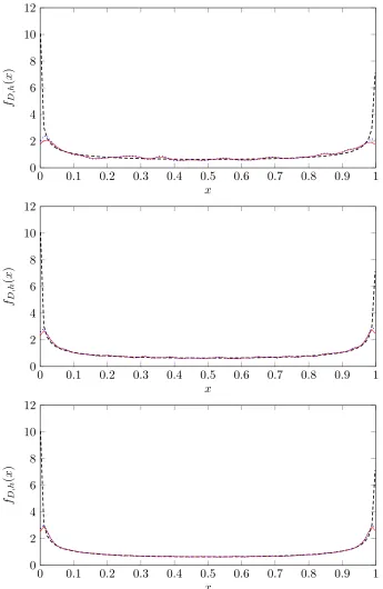
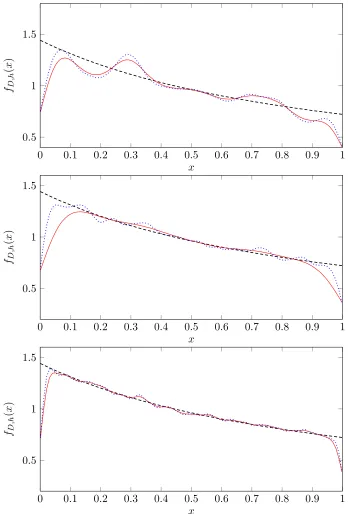
In Figs. 1 and 2, we also plot the kernel density estimators for Logistic map in Example 2 and Gauss map in Example 3 with different bandwidths and their true density functions with different sample sizes. The sample size of each panel, in Figs. 1 and 2, from up to bottom, is 103, 104, and 105, respectively. In each panel, the densely dashed black curve represents the true density, the dotted blue curve is the estimated density function with the bandwidth selected by the baseline method while the solid red curve stands for the estimated density with the bandwidth selected by the double kernel method. All density functions in Figs. 1 and 2 are plotted with 100 equispaced points in the interval (0,1).
0 0.1 0.2 0.3 0.4 0.5 0.6 0.7 0.8 0.9 1 0
2 4 6 8 10 12
x fD
,h
(
x
)
0 0.1 0.2 0.3 0.4 0.5 0.6 0.7 0.8 0.9 1 0
2 4 6 8 10 12
x fD
,h
(
x
)
0 0.1 0.2 0.3 0.4 0.5 0.6 0.7 0.8 0.9 1 0
2 4 6 8 10 12
x fD
,h
(
x
)
Figure 1: Plots of the kernel density estimatorsfD,hfor Logistic map in Example 2 with different bandwidths
and its true density with different sample sizes. The sample size of each panel, from up to bottom, is 103, 104, and 105, respectively. In each panel, the dashed black curve represents the true
0 0.1 0.2 0.3 0.4 0.5 0.6 0.7 0.8 0.9 1 0.5
1 1.5
x fD
,h
(
x
)
0 0.1 0.2 0.3 0.4 0.5 0.6 0.7 0.8 0.9 1 0.5
1 1.5
x fD
,h
(
x
)
0 0.1 0.2 0.3 0.4 0.5 0.6 0.7 0.8 0.9 1 0.5
1 1.5
x fD
,h
(
x
)
Figure 2: Plots of the kernel density estimatorsfD,hfor Gauss map in Example 3 with different bandwidths
and its true density with different sample sizes. The sample size of each panel, from up to bottom, is 103, 104, and 105, respectively. In each panel, the dashed black curve represents the true density
Table 1: The AMEs of Different Bandwidth Selectors for Logistic Map in Example 2
sample size LSCV MLSCV-1 MLSCV-2 DKM Baseline
5×10² .3372 .3369 .3372 .3117 .3013
1×10³ .2994 .2994 .2994 .2804 .2770
5×10³ .2422 .2422 .2422 .2340 .2326
1×10⁴ .2235 .2235 .2235 .2220 .2192
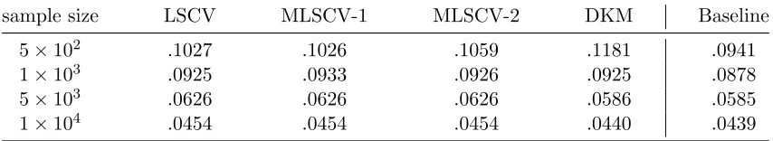
Table 2: The AMEs of Different Bandwidth Selectors for Gauss Map in Example 3
sample size LSCV MLSCV-1 MLSCV-2 DKM Baseline
5×10² .1027 .1026 .1059 .1181 .0941
1×10³ .0925 .0933 .0926 .0925 .0878
5×10³ .0626 .0626 .0626 .0586 .0585
1×10⁴ .0454 .0454 .0454 .0440 .0439
is, for existing bandwidth selectors, there seems no a universal optimal one that can be applicable to all dynamical systems and outperforms the others. Therefore, further explo-ration and insights on the bandwidth selection problem in the dynamical system context certainly deserve future study. On the other hand, we also notice that due to the presence of dependence among observations generated by dynamical systems, the sample size usually needs to be large enough to approximate the density function well. This can be also seen from the plotted density functions in Figs. 1 and 2 with varying sample sizes.
Aside from the above observations, not surprisingly, from Figs. 1 and 2, we also observe the boundary effect (Gasser et al., 1985) from the kernel density estimators for dynamical systems, which seems to be even more significant than the i.i.d case. From a practical implementation view, some special studies are arguably called for addressing this problem.
6. Proofs
The following lemma is needed for the proof of Example 2.
Lemma 16 Forx, h≥0 with x≥2h and p∈(0,1) we have x−h≥2p−1x1−php.
Proof [of Lemma 16] For c:= 2p−1,x≥0, andh≥0 we definegh(x) :=cx1−php−x+h,
so that our goal is to showgh(x)≤0 for allx≥2h. To this end, we first note that
gh(2h) =c(2h)1−php−h=c21−ph1−php−h= 0,
that is, the assertion is true for x= 2h. To show the inequality for x >2h, we note that
g0h(x) = (1−p)cx−php −1. A simple calculation then shows that g0h has its only zero at
x∗ := ((1−p)c)1/ph. Moreover, sincegh00(x) = (1−p)(−p)cx−1−php<0 we see thatgh has a
so that it suffices to show thatx∗≤2h. The latter, however is equivalent to (1−p)c≤2p, and by the definition of c, this inequality is satisfied if and only if (1−p)/2≤1. Since the latter is obviously true, we obtain the assertion.
Proof [of Example 2] Here we only need to show that the density f isα-controllable with the specified functions. Moreover, this is obvious for x <0 and x > 1. Moreover, the first and second derivatives of f on (1/8,7/8) are
f0(x) =− 1−2x
2π(x(1−x))3/2 and f
00(x) = 8x2−8x+ 3 4π(x(1−x))5/2 .
Clearly, this givesf00(x)≥1 for allx∈(1/8,7/8) and hencef0 is increasing on this interval. Using the symmetry off0 aroundx= 1/2 we then obtain
sup
x∈(1/8,7/8
|f0(x)|=|f0(1/8)|= 3 8π ·
64
7
3/2 ≤4.
Consequently, the restriction f|[1/8,7/8] is Lipschitz continuous with constant not exceeding
4. This shows the assertion for x∈ [1/4,3/4]. Therefore, it remains to consider the cases 0< x <1/4 and 3/4< x <1, and due to the symmetry of f we may actually restrict our considerations to 0< x <1/4. Let us therefore fix anx∈(0,1/4). Forh with|h|< r(x), that is h∈(−x/2, x/2), we then find
π|f(x+h)−f(x)|=
p
x(1−x)−p(x+h)(1−x−h) p
x(1−x)(1−x−h)(x+h) . (18)
Moreover, we have 1−x >3/4 and 1−x−h >5/8 and hence we find
1
p
x(x+h)(1−x−h)(1−x) ≤
r
32 15 ·
1
p
x(x+h). (19)
Our next goal is to bound the numerator in (18). To this end, we define
g(x, h) :=px(1−x)−p(x+h)(1−x−h), h, x∈[0,1/4].
Note that the functiont7→pt(1−t) is increasing on [0,1/2] and hence we haveg(x, h)≥0 ifh∈[−1/4,0] andg(x, h)≤0 ifh∈[0,1/4]. Now, our goal is to establish
g(x, h)
≤ |h|1/2, x∈[0,1/4], h∈(−x/2,1/4] (20)
In the caseh∈[0,1/4] our preliminary considerations on gshow that (20) is equivalent to
(x+h)(1−x−h)≤h+x(1−x) + 2phx(1−x).
Moreover, simple algebraic transformations show that the latter is equivalent to−2xh−h2≤
2phx(1−x), which is obviously true. This shows (20) for h ∈[0,1/4]. Now, in the case
h∈(−x/2,0] we first observe that we have
g(x, h)
=
Let us write ˜x := x+h and ˜h := −h. Then we have ˜h ∈ [0, x/2) ⊂ [0,1/4] and ˜x ∈
(x/2, x]⊂(0,1/4]. Using (20) in the already proven case ˜h∈[0,1/4] we then find
g(x, h)
=
g(˜x,˜h)
≤ |˜h|1/2 =|h|1/2,
which finishes the proof of (20).
Now combining (19) with (20) we find
π|f(x+h)−f(x)| ≤ r
32 15 ·
p |h| p
x(x+h).
Let us first consider the caseh∈(−x/2,0]. Then Lemma 16 applied top:= 2εand ˜h:=−h
gives
1
√
x+h =
1
p
x−˜h
≤2(1−p)/2x(p−1)/2˜h−p/2= 21/2−εx−1/2+ε|h|−ε
Inserting this inequality in the previous inequality thus shows
|f(x+h)−f(x)| ≤ 1
π ·
r
64 15 ·x
−1+ε|h|1/2−ε≤x−1+ε|h|1/2−ε. (21)
Moreover, forh∈[0, x/2) we havex+h≥x−h, and hence the previous considerations actu-ally give (21) for allh∈(−x/2, x/2). Since forε:= 1/2−αwe have both−1+ε=−1/2−α
and 1/2−ε=α, we then obtain the assertion.
The following lemma, which will be used several times in the sequel, supplies the key to the proof of Propositions 11 and 10.
Lemma 17 Assume that K is a d-dimensional smoothing kernel that satisfies Condition
(ii) of Assumption B. Then there exists a constant c1 >0 such that for all r >0 we have
Z
Bc r
K(kxk) dx≤c1r−υ. (22) Moreover, for all probability measures Q onRd and all h >0 and r >0 the functions kx,h, which are defined in (12) for all x∈Rd, satisfy
Z
Bc r
EQkx,hdx≤κ Q(Br/2c ) +c12υ(h/r)υ. (23) Proof [of Lemma 17] For the proof of (22) we fix a constant ˜c ≥ 1 such that we have ˜
c−1k · k `d
2 ≤ k · k ≤c˜k · k`d2. SinceK is monotonically decreasing, we then find
Z
Bc r
K(kxk) dx≤ Z
Bc r
K(˜c−1kxk`d
2) dx≤
Z ∞
˜ c−1r
K(˜c−1t)td−1dt
= ˜cd
Z ∞
˜ c−2r
K(t)td−1dt
≤˜cd+2υ
Z ∞
˜ c−2r
K(t)r−υtd+υ−1dt
where in the last step we used Condition (ii) of Assumption B. For the proof of (23) we first observe that for t0>0, we have
Z
Bc r
EQkx,hdx=
Z
Bc r
Z
Rd
h−dK kx−x0k/h dQ(x0) dx
=
Z
Rd Z
Rd
K(kxk)1Bc
r(hx+x
0
) dxdQ(x0)
=
Z
Rd
K(kxk)
Z
Rd
1Bc
r(hx+x
0
) dQ(x0) dx
≤ Z
Bt0
K(kxk)
Z
Rd
1Bc
r(hx+x
0
) dQ(x0)dx+
Z
Bc t0
K(kxk) dx.
Moreover, it is easy to see that 1Bc
r(hx+x
0) = 1 if and only if khx+x0k ≥r. Now we set
t0 := 2hr . In this case, if we additionally havex∈Bt0, thenkx
0k ≥r−hkxk ≥r−ht
0 =r/2.
Using (22) we thus find
Z
Bc r
EQkx,hdx≤
Z
Bt0
K(kxk)Q(Br/2c ) dx+
Z
Bc t0
K(kxk) dx
≤κ Q(Br/2c ) +c1t−0υ. (24)
By t0= 2hr we then find the assertion.
The following technical lemma is needed in the proof of Proposition 10.
Lemma 18 For all 0≤a≤b and d≥1 we have
bd−ad≤d·bd−1·(b−a). (25)
Proof [of Lemma 18] In the case b = 0 there is nothing to prove. Moreover, in the case
b >0, we first observe by deviding by bdthat (25) is equivalent to
1−a
b
d
≤d·1−a
b
.
Consequently, it suffices to show
1−td≤d(1−t), t∈[0,1]. (26)
To this end, we define h(t) =d(1−t)−1 +td fort∈[0,1]. This gives h0(t) =−d+dtd−1
and a simple check then showsh0(t) ≤0 for all t∈[0,1]. Moreover, we have h(1) = 0 and combining both we thus findh(t)≥0 for allt∈[0,1]. This shows (26).
Proof [of Proposition 10] (i). Since the space of continuous and compactly supported functions Cc(Rd) is dense inL1(Rd), we can find ¯f ∈Cc(Rd) such that
Therefore, for any ε >0, we have
kfP,h−fk1=
Z
Rd
|f∗Kh−f|dx
≤ Z
Rd
|f∗Kh−f¯∗Kh|dx+
Z
Rd
|f¯∗Kh−f¯|dx+
Z
Rd
|f −f¯|dx
≤ 2ε
3 +
Z
Rd
|f¯∗Kh−f¯|dx,
(27)
whereKh is defined in (6) and the last inequality follows from the fact that
kf∗Kh−f¯∗Khk1 ≤ kf −f¯k1 ≤ε/3.
The above inequality is due to Young’s inequality (8.7) in Folland (1999). Moreover, there exist a constantM >0 such that supp( ¯f)⊂BM and a constantr >0 such that
Z
Bc r
K(kxk) dx≤ ε
9kf¯k1 .
Now we define L:Rd→[0,∞) by
L(x) :=1[−r,r](kxk)K(kxk)
and Lh :Rd→[0,∞) by
Lh(x) :=h−dL(x/h).
Then we have
Z
Rd
|f¯∗Kh−f¯|dx≤
Z
Rd
|f¯∗Kh−f¯∗Lh|dx+
Z
Rd
|f¯∗Lh−f¯|dx
≤ kf¯k1kKh−Lhk1+
Z Rd ¯
f ∗Lh−f¯
Z
Rd
Lhdx
dx + Z Rd ¯ f ∗ Z Rd
(Lh−Kh) dx
dx
≤2kf¯k1kKh−Lhk1+
Z Rd ¯
f∗Lh−f¯
Z
Rd
Lhdx
dx.
Moreover, we have
kKh−Lhk1 =
Z Rd 1 hd
1[−r,r]
k xk h K k xk h −K k xk h dx = Z Rd
1[−r,r](kxk)K(kxk)−K(kxk) dx = Z Bc r
K(kxk) dx≤ ε
Finally, for h≤1, we have Z Rd ¯
f ∗Lh−f¯
Z
Rd
Lhdx
dx=
Z Rd Z Rd ¯
f(x−x0)−f¯(x)
Lh(x0) dx0
dx ≤ Z
Br+M
Z
Rd
|f¯(x−x0)−f¯(x)|Lh(x0) dx0dx.
Since ¯f is uniformly continuous, there exists a constanthε>0 such that for allh≤hε and
kx0k ≤rh, we have
|f¯(x−x0)−f¯(x)| ≤ε0 := ε 9(r+M)dλd(B
1) .
Consequently we obtain
Z
Rd
|f¯(x−x0)−f¯(x)|Lh(x0) dx0≤ε0
Z
Brh
Lh(x0) dx0≤ε0
Z
Rd
Khdx=ε0.
Therefore, we obtain
Z Rd ¯
f ∗Lh−f¯
Z
Rd
Lhdx
dx≤ Z
Br+M
ε0dx= ε
9 (28)
and consequently the assertion can be proved by combining estimates in (27) and (28).
(ii). The α-H¨older continuity of f tells us that for anyx∈Rd, there holds
|fP,h(x)−f(x)|=
1 hd Z Rd K k
x−x0k
h
f(x0) dx0−f(x)
= Z Rd
K(kx0k)f(x+hx0) dx0−f(x)
= Z Rd
K(kx0k) f(x+hx0)−f(x)dx0
≤c1
Z
Rd
K(kx0k) hkx0kα
dx0
≤c2
Z
Rd
K kx0k`d
2
hαkx0kα`d
2
dx0
≤c3hα
Z ∞
0
K(r)rα+d−1dr
≤c3καhα,
wherec1, c2, c3 >0 are suitable constants. (iii). For fixedh >0 we definer := r0
2h. A quick calculation then yieldshr=r0/2< r0.