Adaptive False Discovery Rate Control under Independence and
Dependence
Gilles Blanchard [email protected]
Weierstraß Institut f¨ur angewandte Analysis und Stochastik Mohrenstrasse 39
10117 Berlin, Germany
´
Etienne Roquain [email protected]
UPMC Univ Paris 06, UMR 7599, Laboratoire de Probabilit´es et Mod`eles Al´eatoires (LPMA) 4 Place Jussieu,
75252 Paris cedex 05, France
Editor: John Shawe-Taylor
Abstract
In the context of multiple hypothesis testing, the proportionπ0of true null hypotheses in the pool of hypotheses to test often plays a crucial role, although it is generally unknown a priori. A testing procedure using an implicit or explicit estimate of this quantity in order to improve its efficency is called adaptive. In this paper, we focus on the issue of false discovery rate (FDR) control and we present new adaptive multiple testing procedures with control of the FDR. In a first part, assuming independence of the p-values, we present two new procedures and give a unified review of other existing adaptive procedures that have provably controlled FDR. We report extensive simulation results comparing these procedures and testing their robustness when the independence assumption is violated. The new proposed procedures appear competitive with existing ones. The overall best, though, is reported to be Storey’s estimator, albeit for a specific parameter setting that does not appear to have been considered before. In a second part, we propose adaptive versions of step-up procedures that have provably controlled FDR under positive dependence and unspecified depen-dence of the p-values, respectively. In the latter case, while simulations only show an improvement over non-adaptive procedures in limited situations, these are to our knowledge among the first the-oretically founded adaptive multiple testing procedures that control the FDR when the p-values are not independent.
Keywords: multiple testing, false discovery rate, adaptive procedure, positive regression depen-dence, p-values
1. Introduction
observed difference. Generally, it is assumed that the natural fluctuation distribution of a single gene is known and the problem is to take into account the number of genes involved (for more details, see for instance Dudoit et al., 2003).
1.1 Adaptive Multiple Testing Procedures
In this work, we focus on building multiple testing procedures with a control of the false discovery rate (FDR). This quantity is defined as the expected proportion of type I errors, that is, the proportion of true null hypotheses among all the null hypotheses that have been rejected (i.e., declared as false) by the procedure. In their seminal work on this topic, Benjamini and Hochberg (1995) proposed the celebrated linear step-up (LSU) procedure, which was proved to control the FDR under the assumption of independence between the p-values. Later, it was proved (Benjamini and Yekutieli, 2001) that the LSU procedure still controls the FDR when the p-values have positive dependence (or more precisely, a specific form of positive dependence called positive regression dependence from a subset, PRDS). Under completely unspecified dependence, the same authors have shown that the FDR control still holds if the threshold collection of the LSU procedure is divided by a factor 1+1/2+···+1/m, where m is the total number of null hypotheses to test. More recently,
the latter result has been generalized (Blanchard and Fleuret, 2007; Blanchard and Roquain, 2008; Sarkar, 2008a,b), by showing that there is in fact a family of step-up procedures (depending on the choice of a kind of prior distribution) that control the FDR under unspecified dependence between the p-values.
However, all of these procedures, which are built in order to control the FDR at a levelα, can be shown to have actually their FDR upper bounded byπ0α, whereπ0is the proportion of true null hypotheses in the initial pool. Therefore, when most of the hypotheses are false (i.e.,π0is small), these procedures are inevitably conservative, since their FDR is in actuality much lower than the fixed targetα. In this context, the challenge of adaptive control of the FDR (e.g., Benjamini and Hochberg, 2000; Black, 2004) is to integrate an estimation of the unknown proportion π0 in the threshold of the previous procedures and to prove that the corresponding FDR is still rigorously controlled byα.
Of course, adaptive procedures are of practical interest if it is expected that π0 is, or can be, significantly smaller than 1. An example of such a situation occurs when using hierarchical pro-cedures (e.g., Benjamini and Heller, 2007) which first selects some clusters of hypotheses that are likely to contain false nulls, and then apply a multiple testing procedure on the selected hypotheses. Since a large part of the true null hypotheses is expected to be false in the second step, an adaptive procedure is needed in order to keep the FDR close to the target level.
A number of adaptive procedures have been proposed in the recent literature and can loosely be divided into the following categories:
• plug-in procedures, where some initial estimator of π0 is directly plugged in as a
• two-stage procedures: in this approach, a first round of multiple hypothesis testing is
per-formed using some fixed algorithm, then the results of this first round are used in order to tune the parameters of a second round in an adaptive way. This can generally be interpreted as using the output of the first stage to estimateπ0. Different procedures following this gen-eral approach have been proposed (Benjamini et al., 2006; Sarkar, 2008a; Farcomeni, 2007); more generally, multiple-stage procedures can be considered.
• one-stage procedures, which perform a single round of multiple testing (generally step-up or
step-down), based on a particular (deterministic) threshold collection that renders it adaptive (Finner et al., 2009; Gavrilov et al., 2009).
In addition, some works (Genovese and Wasserman, 2004; Storey et al., 2004; Finner et al., 2009) have studied the question of adaptivity to the parameterπ0 from an asymptotic viewpoint. In this framework, the more specific random effects model is—most generally, though not always— considered, in which p-values are assumed independent, each hypothesis has a probability π0 of being true, and all false null hypotheses share the same alternate distribution. The behavior of different procedures is then studied under the limit where the number of tested hypotheses grows to infinity. One advantage of this approach and specific model is that it allows to derive quite precise results (see Neuvial, 2008, for a precise study of limiting behaviors of central limit type under this model, including some of the new procedures introduced in the present paper). However, we emphasize that in the present work our focus is decidedly on the nonasymptotic side, using finite samples and arbitrary alternate hypotheses.
To complete this overview, let us also mention another interesting and different direction opened up recently, that of adaptivity to the alternate distribution. If the alternate distributions are known
a priori, the optimal testing statistics are generally likelihood ratios between each null and each
al-ternate, which (possibly after standardization under the form of p-values) can be combined using a multiple testing algorithm in order to control some measure of type I error while minimizing a mea-sure of type II error (see, e.g., Spjøtvoll, 1972, Wasserman and Roeder, 2006, Genovese et al., 2006, Storey, 2007, Roquain and van de Wiel, 2009). In situations where the alternate is unknown, though, one can hope to estimate, implicitly or explicitly, the alternate distributions from the observed data, and consequently approximate the optimal test statistics and the associated multiple testing proce-dure (Sun and Cai, 2007 proposed an asymptotically consistent approach to this end). Interestingly, this point of view is also intimately linked to some traditional topics in statistical learning such as classification and of optimal novelty detection (see, e.g., Scott and Blanchard, 2009). However, in the present paper we will focus on adaptivity to the parameterπ0only.
1.2 Overview of this Paper
The contributions of the present paper are the following. A first goal of the paper is to introduce a number of novel adaptive procedures:
2. Based on this, we then build a new two-stage adaptive procedure, which is more powerful in general than the procedure proposed by Benjamini et al. (2006), while provably controlling the FDR under independence.
3. Under the assumption of positive or arbitrary dependence of the p-values, we introduce new two-stage adaptive versions of known step-up procedures (namely, of the LSU under positive dependence, and of the family of procedures introduced by Blanchard and Fleuret, 2007, under unspecified dependence). These adaptive versions provably control the FDR and result in an improvement of power over the non-adaptive versions in some situations (namely, when the number of hypotheses rejected in the first stage is large, typically more than 60%).
A second goal of this work is to present a review of several existing adaptive step-up procedures with provable FDR control under independence. For this, we present the theoretical FDR control as a consequence of a single general theorem, which was first established by Benjamini et al. (2006). Here, we give a short self-contained proof of this result that is of independent interest. The latter is based on some tools introduced earlier (Blanchard and Roquain, 2008; Roquain, 2007), aimed at unifying FDR control proofs. Related results and tools also appear independently in Finner et al. (2009) and Sarkar (2008b).
A third goal is to compare both the existing and our new adaptive procedures in an extensive simulation study under both independence and dependence, following the simulation model and methodology used by Benjamini et al. (2006):
• Concerning the new one- and two- stage procedures with theoretical FDR control under in-dependence, these are generally quite competitive in comparison to existing ones. However we also report that the best procedure overall (in terms of power, among procedures that are robust enough to the dependent case) appears to be the plug-in procedure based on the well-known Storey estimator (Storey, 2002) used with the somewhat nonstandard parameter setting
λ=α. This outcome was in part unexpected since to the best of our knowledge, this fact had never been pointed out so far (the usual default recommended choice isλ=1
2 and turns out to be very unstable in dependent situations); this is therefore an important conclusion of this paper regarding practical use of these procedures.
• Concerning the new two-stage procedures with theoretical FDR control under dependence, simulations show an (admittedly limited) improvement over their non-adaptive counterparts in favorable situations which correspond to what was expected from the theoretical study (i.e., large proportion of false hypotheses). The observed improvement is unfortunately not striking enough to be able to recommend using these procedures in practice.
2. Preliminaries
In this paper, we stick to the traditional statistical framework for multiple testing, which we first briefly recall below.
2.1 Multiple Testing Framework
Let(
X
,X,P)be a probability space; we aim at inferring a decision onPfrom an observation x inX
drawn fromP. LetH
be a finite set of null hypotheses forP, that is, each null hypothesis h∈H
corresponds to some subset of distributions on(X
,X)and “Psatisfies h” means thatPbelongs to this subset of distributions. The number of null hypotheses|H
|is denoted by m, where|.|is the car-dinality function. The underlying probabilityPbeing fixed, we denoteH
0={h∈H
|Psatisfies h} the set of the true null hypotheses and m0=|H
0|the number of true null hypotheses. We let alsoπ0:=m0/m the proportion of true null hypotheses. We stress that
H
0, m0, andπ0are unknown andimplicitly depend on the unknownP. All the results to come are always implicitly meant to hold for any generating distributionP.
We suppose further that there exists a set of p-value functions p= (ph,h∈
H
), meaning that each ph:(X
,X)7→[0,1]is a measurable function and that for each h∈H
0, phis bounded stochas-tically by a uniform distribution, that is,∀h∈
H
0, ∀t∈[0,1],P[ph≤t]≤t. (1) Typically, each p-value is obtained from a statistic Z that has a known distribution P0 under the corresponding null hypothesis. In this case, ph =Φ0(Z) satisfies (1) in general, where Φ0(z) =P0([z,+∞)). Here, we are however not concerned with how these p-values are precisely constructed and only assume that they exist and are known (this is the standard setting in multiple testing).
2.2 Multiple Testing Procedure and Errors
A multiple testing procedure is a function
R : x∈
X
7→R(x)∈P
(H
),such that for any h∈
H
, the function x7→1{h∈R(x)}is measurable. It takes as input an observa-tion x and returns a subset ofH
, corresponding to the rejected hypotheses. As it is commonly the case, we will focus here on multiple testing procedure based on p-values, that is, we will implicitly assume that R is of the form R(p).A multiple testing procedure R can make two kinds of errors: a type I error occurs for h when
h is true and is rejected by R , that is, h∈
H
0∩R. Conversely, a type II error occurs for h whenh is false and is not rejected by R, that is h∈
H
cMore recently, a more liberal measure of type I errors has been introduced in multiple testing (Ben-jamini and Hochberg, 1995): the false discovery rate (FDR), which is the averaged proportion of true null hypotheses in the set of all the rejected hypotheses:
Definition 1 (False discovery rate) The false discovery rate of a multiple testing procedure R for
a generating distributionPis given by
FDR(R):=E
|R∩
H
0||R| 1{|R|>0}
. (2)
A classical aim, then, is to build procedures R with FDR upper bounded at a given, fixed level
α. Of course, if we choose R=/0, meaning that R rejects no hypotheses, trivially FDR(R) =0≤α. Therefore, it is desirable to build procedures R satisfying FDR(R)≤α while at the same time having as few type II errors as possible. As a general rule, provided that FDR(R)≤α, we want to build procedures that reject as many false hypotheses as possible. The absolute power of a multiple testing procedure is defined as the average proportion of false hypotheses correctly rejected,
ER∩
H
c 0/
H
c0
. Given two procedures R and R′, a particularly simple sufficient condition for
R to be more powerful than R′is when R′if R′⊂R holds pointwise. We will say in this case that R
is (uniformly) less conservative than R′.
Remark 2 Throughout this paper we will use the following convention: whenever there is an
in-dicator function inside an expectation, this has logical priority over any other factor appearing in the expectation. What we mean is that if other factors include expressions that may not be defined
(such as the ratio 00) outside of the set defined by the indicator, this is safely ignored. This results in
more compact notation, such as in Definition 1. Note also again that the dependence of the FDR on
the unknownPis implicit.
2.3 Self-Consistency, Step-Up Procedures, FDR Control and Adaptivity
We first define a general class of multiple testing procedures called self-consistent procedures (Blan-chard and Roquain, 2008).
Definition 3 (Self-consistency, nonincreasing procedure) Let∆:{0,1, . . . ,m} →R+,∆(0) =0 ,
be a nondecreasing function called threshold collection; a multiple testing procedure R is said to
satisfy the self-consistency condition with respect to∆if the inclusion
R⊂ {h∈
H
|ph≤∆(|R|)}holds almost surely. Furthermore, we say that R is nonincreasing if for all h∈
H
the functionph7→ |R(p)|is nonincreasing, that is if|R|is nonincreasing in each p-value.
The class of self-consistent procedures includes well-known types of procedures, notably step-up and step-down. The assumption that a procedure is nonincreasing, which is required in addition to self-consistency in some of the results to come, is relatively natural as a lower p-value means we have more evidence to reject the corresponding hypothesis. We will mainly focus on the step-up procedure, which we define now. For this, we sort the p-values in increasing order using the notation
p(1)≤ ··· ≤p(m)and putting p(0)=0 . This order is of course itself random since it depends on the
Definition 4 (Step-up procedure) The step-up procedure with threshold collection∆is defined as
R={h∈
H
|ph≤p(k)}, where k=max{0≤i≤m|p(i)≤∆(i)}.A trivial but important property of a step-up procedure is the following.
Lemma 5 The step-up procedure with threshold collection∆is nonincreasing and self-consistent
with respect to∆.
Therefore, a result valid for any nonincreasing self-consistent procedure w.r.t.∆holds in particular for the corresponding step-up procedure. This will be used extensively through the paper and thus should be kept in mind by the reader.
Among all procedures that are self-consistent with respect to∆, the step-up is uniformly less conservative than any other (Blanchard and Roquain, 2008) and is therefore of primary interest. However, to recover procedures of a more general form (including step-down for instance), the statements of this paper will be preferably expressed in terms of self-consistent procedures when it is possible.
Threshold collections are generally scaled by the target FDR level α. Once correspondingly rewritten under the normalized form∆(i) =αβ(i)/m , we will callβthe shape function for threshold collection∆. In the particular case where the shape functionβis the identity function, the procedure is called the linear step-up (LSU) procedure (at levelα).
The LSU plays a prominent role in multiple testing for FDR control; it was the first procedure for which FDR control was proved and it is probably the most widely used procedure in this context. More precisely, when the p-values are assumed to be independent, the following theorem holds.
Theorem 6 Suppose that the family of p-values p= (ph,h∈
H
)is independent. Then anynonin-creasing self-consistent procedure with respect to threshold collection∆(i) =αi/m has FDR upper
bounded byπ0α, whereπ0=m0/m is the proportion of true null hypotheses. (In particular, this
is the case for the linear step-up procedure.) Moreover, if the p-values associated to true null hy-potheses are exactly distributed like a uniform distribution, the linear step-up procedure has FDR
exactly equal toπ0α.
For the specific case of the LSU, the first part of this result was proved in the landmark paper of Benjamini and Hochberg (1995); the second part was proved by Benjamini and Yekutieli (2001) and Finner and Roters (2001). Benjamini and Yekutieli (2001) extended the first part by proving that the LSU procedure still controls the FDR in the case of p-values with a certain form of pos-itive dependence called pospos-itive regression dependence from a subset (PRDS). We skip a formal definition for now (we will get back to this topic in Section 4). The extension of these results to self-consistent procedures (in the independent as well as PRDS case) was established by Blanchard and Roquain (2008) and Finner et al. (2009).
However, when no particular assumption is made on the dependence between the p-values, it can be shown that the above FDR control does not hold in general. This situation is called
unspecified or arbitrary dependence. A modification of the LSU was first proposed by Benjamini
Theorem 7 Under unspecified dependence of the family of p-values p= (ph,h∈
H
), letβ be ashape function of the form:
β(r) =
Z r
0
udν(u), (3)
whereνis some fixed a priori probability distribution on(0,∞). Then any self-consistent procedure
with respect to threshold collection∆(i) =αβ(i)/m has FDR upper bounded byαπ0.
To recap, in all of the above cases, the FDR is actually controlled at the levelπ0αinstead of the targetα. Hence, a direct corollary of both of the above theorems is that the step-up procedure with shape functionβ∗(x) =π0−1β(x)has FDR upper bounded byαin either of the following situations:
- β(x) =x when the p-value family is independent or PRDS,
- the shape functionβis of the form (3) when the p-values have unspecified dependence.
Sinceπ0≤1, usingβ∗always gives rise to a less conservative procedure than usingβ(especially whenπ0is small). However, sinceπ0is unknown, the shape functionβ∗is not directly accessible. We therefore call the step-up procedure using β∗ the Oracle step-up procedure based on shape functionβ(in each of the above cases).
Simply put, the role of adaptive step-up procedures is to mimic the latter oracle in order to obtain more powerful procedures. Adaptive procedures are often step-up procedures using the modified shape function Gβ, where G is some estimator ofπ−01:
Definition 8 (Plug-in adaptive step-up procedure) Given a level α∈(0,1), a shape function β
and an estimator G :[0,1]H →(0,∞)of the quantityπ−01, the plug-in adaptive step-up procedure
of shape functionβand using estimator G (at levelα) is defined as
R={h∈
H
|ph≤p(k)}, where k=max{0≤i≤m|p(i)≤αβ(i)G(p)/m}.The (data-dependent) function∆(p,i) =αβ(i)G(p)/m is called the adaptive threshold collection
corresponding to the procedure. In the particular case where the shape functionβ is the identity
function onR+, the procedure is called an adaptive linear step-up procedure using estimator G
(and at levelα).
Following the previous definition, an adaptive plug-in procedure is composed of two different steps:
1. Estimateπ−01with an estimator G .
2. Take the step-up procedure of shape function Gβ.
A subclass of plug-in adaptive procedures is formed by so-called two-stage procedures, when the estimator G is actually based on a first, non-adaptive, multiple testing procedure. This can obviously be possibly iterated and leads to multi-stage procedures. The distinction between generic plug-in procedures and two-stage procedures is somewhat informal and generally meant only to provide some kind of nomenclature between different possible approaches.
3. Adaptive Procedures with Provable FDR Control under Independence
In this section, we introduce two new adaptive procedures that provably control the FDR under independence. The first one is one-stage and does not include an explicit estimator ofπ−01, hence it is not explicitly a plug-in procedure. We then propose to use this as the first stage in a new two-stage procedure, which constitutes the second proposed method.
For clarity, we first introduce the new one-stage procedure; we then discuss several possible plug-in procedures, including our new proposition and several procedures proposed by other au-thors. FDR control for these various plug-in procedures can be studied under independence using a general theoretical device introduced by Benjamini et al. (2006) which we reproduce here with a self-contained and somewhat simplified proof. Finally, we compare these different approaches; first with a theoretical study of the robustness under a very specific case of maximal dependence; second by extensive simulations, where we inspect both the performance under independence and the robustness under a wide range of positive correlations.
3.1 New Adaptive One-Stage Step-Up Procedure
We present here our first main contribution, a one-stage adaptive step-up procedure. This means that the estimation step is implicitly included in the (deterministic) threshold collection.
Theorem 9 Suppose that the p-value family p= (ph,h∈
H
)is independent and letλ∈(0,1) befixed. Define the adaptive threshold collection
∆(i) =min
(1−λ) αi
m−i+1,λ
. (4)
Then any nonincreasing self-consistent procedure with respect to∆has FDR upper bounded byα.
In particular, this is the case of the corresponding step-up procedure, denoted by BR-1S-λ.
The above result is proved in Section 6. Our proof is in part based on Lemma 1 of Benjamini et al. (2006). Note that an alternate proof of Theorem 9 is established in Sarkar (2008b) without using this lemma, while nicely connecting the FDR upper-bound to the false non-discovery rate.
3.1.1 COMPARISON TO THELSU
Below, we will mainly focus on the choiceλ=α, leading to the threshold collection
∆(i) =αmin
(1−α) i
m−i+1,1
. (5)
For i≤(m+1)/2, the threshold (5) is αm(1−−αi+)1i,and thus our approach differs from the threshold collection of the standard LSU procedure threshold by the factor (m1−α−i+)m1.
It is interesting to note that the correction factor m−mi+1 appears in Holm’s step-down procedure (Holm, 1979) for FWER control. The latter is a well-known improvement of Bonferroni’s procedure (which corresponds to the fixed thresholdα/m), taking into account the proportion of true nulls, and
defined as the step-down procedure1 with threshold collectionα/(m−i+1). Here we therefore
1. The step-down procedure with threshold collection∆rejects the hypotheses corresponding to the k smallest p-values,
prove that this correction is suitable as well for the linear step-up procedure, in the framework of FDR control.
If r denotes the final number of rejections of the new one-stage procedure, we can interpret the ratio (m1−α−r+)m1 between the adaptive threshold and the LSU threshold at the same point as an a
posteriori estimate forπ−01. In the next section we propose to use this quantity in a plug-in,
two-stage adaptive procedure.
As Figure 1 illustrates, our procedure is generally less conservative than the (non-adaptive) linear step-up procedure (LSU). Precisely, the new procedure can only be more conservative than the LSU procedure in the marginal case where the factor (m1−α−i+)m1 is smaller than one. This happens only when the proportion of null hypotheses rejected by the LSU procedure is positive but less
thanα+1/m (and even in this region the ratio of the two threshold collections is never less than
(1−α)). Roughly speaking, this situation with only few rejections can only happen if there are few false hypotheses to begin with (π0close to 1) or if the false hypotheses are very difficult to detect (the distribution of false p-values is close to being uniform).
In the interest of being more specific, we briefly investigate this issue in the next lemma, con-sidering the particular Gaussian random effects model (which is relatively standard in the multiple testing literature, see, for example, Genovese and Wasserman, 2004) in order to give a quantitative answer from an asymptotical point of view (when the number of tested hypotheses grows to infinity). In the random effect model, hypotheses are assumed to be randomly true or false with probability
π0, and the false null hypotheses share a common distribution P1. Globally, the p-values then are i.i.d. drawn according to the mixture distributionπ0U[0,1] + (1−π0)P1.
0 0.05 0.1 0.15 0.2
0 200 400 600 800 1000
LSU AORC BR-1S,λ=α BR-1S,λ=2α BR-1S,λ=3α FDR09-1/2 FDR09-1/3
Figure 1: For m=1000 null hypotheses andα=5%: comparison of the new threshold collection
Lemma 10 Consider the random effects model where the p-values are i.i.d. with common
cumula-tive distribution function t7→π0t+ (1−π0)F(t). Assume that the true null hypotheses are standard
Gaussian with zero mean and that the alternative hypotheses are standard Gaussian with mean µ>0 . In this case F(t) =Φ(Φ−1(t)−µ), where Φis the standard Gaussian upper tail function.
Assumingπ0<(1+α)−1, define
µ⋆=Φ−1(α2)−Φ−1
α−1
−π0 1−π0
α2
.
Then if µ>µ∗, the probability that the LSU rejects a proportion of null hypotheses less than 1/m+α
tends to 0 as m tends to infinity. On the other hand, ifπ0>(1+α)−1, or µ<µ∗, then this probability
tends to one.
Lemma 10 is proved in Section 6. Taking for instance in this lemma the values π0=0.5 and
α=0.05, results in the critical value µ⋆≃1.51 . This lemma delineates clearly in a particular case in which situation we can expect an improvement from the adaptive procedure BR-1S over the standard LSU.
3.1.2 COMPARISON TOOTHERADAPTIVE ONE-STAGEPROCEDURES
Very recently, other adaptive one-stage procedures with important similarities to BR-1S-λhave been proposed by other authors. (The present work was developed independently.)
Starting with some heuristic motivations, Finner et al. (2009) proposed the threshold collection
t(i) = m−(αi1−α)i, which they dubbed the asymptotically optimal rejection curve (AORC). However, the step-up procedure using this threshold collection as is does not have controlled FDR (since
t(m) =1 , the corresponding step-up procedure would always reject all the hypotheses), and several suitable modifications were proposed by Finner et al. (2009), the simplest one being
tη′(i) =min t(i),η−1αi/m,
which is denoted by FDR09-ηin the following.
The theoretical FDR control proved in Finner et al. (2009) is studied asymptotically as the number of hypotheses grows to infinity. In that framework, asymptotical control at levelαis shown to hold for any η<1. On Figure 1, we represented the thresholds BR-1S-λ and FDR09-η for comparison, for several choices of the parameters. The two families appear quite similar, initially following the AORC curve, then branching out or capping at a point depending on the parameter. One noticeable difference in the initial part of the curve is that while FDR09-ηexactly coincides with the AORC, BR-1S-λis arguably sligthly more conservative. This reflects the nature of the corresponding theoretical result—nonasymptotic control of the FDR requires a somewhat more conservative threshold as compared to the only asymptotic control of FDR-η. Additionally, we can use BR-1S-λas a first step in a 2-step procedure, as will be argued in the next section.
The ratio between BR-1S-λand the AORC (before the capping point) is a factor which, assuming
α≥(m+1)−1, is lower bounded by(1−λ)(1− 1
m+1). This suggests that the value forλshould be kept small, this is why we proposeλ=α as a default choice.
Finally, the step-down procedure based on the AORC threshold collection (under the slightly modified formet(i) = m αi
3.2 Adaptive Plug-In Methods
In this section, we consider different adaptive step-up procedures of the plug-in type, that is, based on an explicit estimator ofπ−01. We first review a general method proposed by Benjamini et al. (2006) in order to derive FDR control for such plug-in procedures (see also Theorem 4.3 of Finner et al., 2009, for a similar result, as well as Theorem 3.3 of Sarkar, 2008b). We propose here a self-contained proof of this result, which notably extends the original result from step-up procedures to more general self-consistent procedures. Based on this result, we review the different plug-in estimators considered by Benjamini et al. (2006) and add a new one to the lot, based on the one-stage adaptive procedure introduced in the previous section.
Let us first introduce the following notation: for each h∈
H
, we denote by p−h the collection of p-values p restricted toH
\ {h}, that is, p−h= (ph′,h′6=h). We also denote p0,h= (p−h,0)thecollection p where phhas been replaced by 0.
Theorem 11 (Benjamini, Krieger, Yekutieli 2006) Suppose that the p-value family p= (ph,h∈
H
)is independent. Let G :[0,1]H →(0,∞)be a measurable, coordinate-wise nonincreasingfunc-tion. Consider a nonincreasing multiple testing procedure R which is self-consistent with respect to
the adaptive linear threshold collection∆(p,i) =αG(p)i/m . Then the following holds:
FDR(R)≤ α
m
∑
h∈H0
E[G(p0,h)]. (6)
In particular, if for any h∈
H
0, it holds thatE[G(p0,h)]≤π−01, then FDR(R)≤α.The proof is given in Section 6. Since we assumed G to be nonincreasing, the quantityE[G(p0,h)] in bound (6) is maximized when the p-values associated to true nulls have a uniform distribution (ph excepted), while the p-values associated to false nulls are all set to zero. Following Finner et al. (2009), this least favorable configuration for the distribution of p-values is referred to as the Dirac-Uniform distribution and gives rise to the following corollary:
Corollary 12 Consider the same conditions as for Theorem 11, and assume moreover that G is
invariant by permutation of the p-values. Then it holds that
FDR(R)≤γ(G,m)α,
withγ(G,m) = max
1≤m0≤m
m0
mEp∼DU(m,m0−1)[G(p)]
,where DU(m,j)is the distribution of p where
the j first p-values are independent uniform in[0,1]and the m−j others are identically equal to
zero.
(While the proof is standard, it is given for completeness in Section 6). The interest of the last result is that for any choice of nonincreasing (permutation invariant) function G , it is possible in principle to evaluateγ(G,m)by a Monte Carlo method, namely by estimating the expected value of
G under the m−1 possible least favorable configurations. This leads to a practical control of the
FDR valid for any value of m0, obtained by dividing the target levelαbyγ(G,m) before applying the procedure.
concentrate on this goal and apply the result of Theorem 11 (or alternatively of Corollary 12) to the following estimators, depending on a fixed parameterλ∈(0,1)or k0∈ {1, . . . ,m}:
[Storey-λ] G1(p) =
(1−λ)m ∑h∈H1{ph>λ}+1
;
[Quant-k0
m] G2(p) =
(1−p(k0))m
m−k0+1
;
[BKY06-λ] G3(p) =
(1−λ)m
m− |R0(p)|+1
,where R0is the standard LSU at levelλ; [BR-2S-λ] G4(p) =
(1−λ)m
m− |R′0(p)|+1,where R ′
0is BR-1S-λ(see Theorem 9).
Above, the notation “Storey-λ”, “Quant-k0
m”, “BKY06-λ” and “BR-2S-λ” refer to the plug-in adap-tive linear step-up procedures associated to G1, G2, G3and G4, respectively.
Estimator G1is usally called modified Storey’s estimator and was initially introduced by Storey (2002) from an heuristics on the p-values histogram (originally without the “+1”, hence the name “modified”). Its intuitive justification is as follows: denoting by Sλthe set of p-values larger than the thresholdλ, the average number of true nulls having a p-value in Sλis m0(1−λ). Hence, a natural estimator of π−01 is (1−λ)m/|Sλ∩
H
0| ≥(1−λ)m/|Sλ| ≃G1(p). In particular, we expect that Storey’s estimator is generally an underestimate ofπ−01, which is in accordance with the condition of Theorem 11. A standard choice isλ=1/2 (as in the SAM software of Storey and Tibshirani, 2003). FDR control for the corresponding plug-in step-up procedure was proved by Storey et al. (2004) (more precisely, for the modificatione∆(p,i) =min(αG1(p)i/m,λ)) and by Benjamini et al. (2006).Estimator G2was introduced by Benjamini and Hochberg (2000) and Efron et al. (2001), from a slope heuristics on the p-values c.d.f. Roughly speaking, G2appears as Storey’s estimator with the data-dependent parameter choiceλ=p(k0), and can therefore be interpreted as the quantile version
of Storey’s estimator. A standard value for k0 is⌊m/2⌋, resulting in the so-called median adaptive LSU (see Benjamini et al., 2006, and the references therein).
Estimator G3was introduced by Benjamini et al. (2006) for the particular choiceλ=α/(1+α). More precisely, a slightly less conservative version, without the “+1” in the denominator, was used in Benjamini et al. (2006). We forget about this refinement here, noting that it results only in a very slight improvement.
Finally, the estimator G4 is new and follows exactly the same philosophy as G3, that is, uses a step-up procedure as a first stage in order to estimate π−01, but this time based on our adaptive one-stage step-up procedure introduced in the previous section, rather than the standard LSU. Note that since R′0 is less conservative than R0 (except in marginal cases), we generally have G3≤G4 pointwise and our estimator improves over the one of Benjamini et al. (2006).
These different estimators all satisfy the sufficient condition mentioned in Theorem 11, and we thus obtain the following corollary:
Corollary 13 Assume that the family of p-values p= (ph,h∈
H
)is independent. For i=1,2,3,4 ,and any h∈
H
0, it holds thatE[Gi(p0,h)]≤π−01. Therefore, the plug-in adaptive linear step-upThe above result for G1, G2 and G3 (for the specific parameter setting λ=α/(1+α)) was proved by Benjamini et al. (2006). In Section 6, we shortly reproduce their arguments, and prove the result for G4.
To sum up, Corollary 13 states that under independence, for anyλand k0, the plug-in adaptive procedures Storey-λ, Quant-k0
m, BKY06-λand BR-2S-λall control the FDR at levelα.
Remark 14 The result proved by Benjamini et al. (2006) is actually slightly sharper than Theorem
11. Namely, if G(·) is moreover supposed to be coordinate-wise left-continuous, it is possible to
prove that Theorem 11 still holds when p0,hin the RHS of (6) is replaced by the slightly bettereph=
(p−h,peh(p−h)), defined as the collection of p-values p where ph has been replaced by eph(p−h) =
maxp∈[0,1]p≤α|R(p−h,p)|G(p−h,p) .This improvement then permits to get rid of the “+1”
in the denominator of G3. Here, we opted for simplicity and a more straightforward statement,
noting that this improvement is not crucial.
Remark 15 The one-stage step-up procedure of Finner et al. (2009) (see previous discussion in
Sec-tion 3.1.2)—for which there is no result proving nonasymptotic FDR control up to our knowledge—
can also be interpreted intuitively as an adaptive version of the LSU using estimator G2, where the
choice of parameter k0 is data-dependent. Namely, assume that we want to reject at least i null
hypotheses whenever p(i)is lower than the standard LSU threshold times the estimator G2 wherein
parameter k0=i is used. This corresponds to the inequality p(i)≤
k(1−p(i))
m−i+1 , which, solved in p(i),
gives the threshold collection of Finner et al. (2009). Remember from Section 3.1.2 that this thresh-old collection must actually be modified in order to be useful, since it otherwise always leads to
reject all hypotheses. The modification leading to FDR09-ηconsists in capping the estimatedπ−01
at a level η, that is, using min(η,G2) instead of G2 in the above reasoning. In fact, the proof
of Finner et al. (2009) relies on a result which is essentially a reformulation of Theorem 11 for a specific form of estimator.
Remark 16 The estimators Gi, i=1,2,3,4 are not necessarily larger than 1, and to this extent
can in some unfavorable cases result in the final procedure being actually more conservative than
the standard LSU. This can only happen in the situation where either π0 is close to 1 (“sparse
signal”) or the alternative hypotheses are difficult to detect (“weak signal”); if such a situation is anticipated, it is more appropriate to use the regular non-adaptive LSU.
For the Storey-λ estimator, we can control precisely the probability that such an unfavorable
case arises by using Hoeffding’s inequality (Hoeffding, 1963): assuming the true nulls are i.i.d.
uniform on(0,1)and the false nulls i.i.d. of c.d.f. F(·), we write by definition of G1
P[G1(p)<1] =P "
1
m
m
∑
h∈H(1{ph>λ} −P[ph>λ])>(1−π0)(F(λ)−λ)−m−1 #
≤exp(−2(mc2+1)),
where we denoted c= (1−π0)(F(λ)−λ), and assumed additionally c>m−1. The behavior of the
bound mainly depends on c , which can get small only ifπ0is close to 1 (sparse signal) or F(λ)is
close toλ(weak signal), illustrating the above point. In general, provided c>0 does not depend
3.3 Theoretical Robustness of the Adaptive Procedures under Maximal Dependence
For the different procedures proposed above, the theory only provides the correct FDR control under independence between the p-values. An important issue is to know how robust this control is when dependence is present (as it is often the case in practice). However, the analytic computation of the FDR under dependence is generally a difficult task, and this issue is often tackled empirically through simulations in a pre-specified model (we will do so in Section 3.4).
In this short section, we present theoretical computations of the FDR for the previously intro-duced adaptive step-up procedures, under the maximally dependent model where all the p-values are in fact equal, that is ph≡p1 for all h∈
H
(and m0=m). It corresponds to the case where we perform m times the same test, with the same p-value. Albeit relatively trivial and limited, this case leads to very simple FDR computations and provides at least some hints concerning the robustness under dependence of the different procedures studied above.Proposition 17 Suppose that we observe m identical p-values p= (p1, ...,pm) = (p1, ...,p1)with
p1∼U([0,1])and assume m=m0. Then, the following holds:
FDR(BR-1S-λ) =min λ,α(1−λ)m,
FDR(FDR09-η) =αη−1,
FDR(Storey-λ) =min λ,α(1−λ)m+ α(1−λ)(1+m−1)−λ+,
FDR(Quant-k0/m) =
α
(1+α)−(k0−1)m−1
,
FDR(BKY06-λ) =FDR(BR-2S-λ) =FDR(Storey-λ).
Interestingly, the above proposition suggests specific choices of the parametersλ, ηand k0to ensure control of the FDR at levelαunder maximal dependence:
• For BR-1S-λ, puttingλ2=α/(α+m−1), Proposition 17 gives that FDR(BR-1S-λ) =λ when-everλ≤λ2. This suggests to takeλ=α, and is thus in accordance with the default choice proposed in Section 3.1.
• For FDR09-η, no choice ofη<1 will lead to the correct FDR control under maximal depen-dence. However, the largerη, the smaller the FDR in this situation. Note that FDR(FDR09-12) = 2α.
• For Storey-λ, BKY06-λand BR-2S-λ, puttingλ1=α/(1+α+m−1), we have FDR=λfor
λ1≤λ≤λ2.This suggests to chooseλ=αwithin these three procedures. Furthermore, note that the standard choiceλ=1/2 for Storey-λ leads to a very poor control under maximal dependence: FDR(Storey-12) =min(αm,1)/2.
• For Quant-k0/m, we see that the value of k0 maximizing the FDR while maintaining it below α is k0 =⌊αm⌋+1. Remark also that the standard choice k0 =⌊m/2⌋ leads to
FDR(Quant-k0/m) =2α/(1+2α+2m−1)≃2α.
but not equal to 1 . For instance, it is well-known that the LSU procedure has FDR far below α for strong positive correlations, but its FDR is equal toα in the above extreme model (see Finner et al., 2007, for a comprehensive study of the LSU under positive dependence). Conversely, the FDR of some adaptive procedures can be higher under moderate dependence than under maximal dependence. This behavior appears in the simulations of the next section, illustrating the complexity of the issue.
3.4 Simulation Study
How can we compare the different adaptive procedures defined above? For a fixed λ, it holds pointwise that G1≥G4≥G3, which shows that the adaptive procedure [Storey-λ] is always less conservative than [BR-2S-λ], itself less conservative than [BKY06-λ] (except in the marginal cases where the one-stage adaptive procedure is more conservative than the standard step-up procedure, as delineated earlier for example in Lemma 10). It would therefore appear that one should always choose [Storey-λ] and disregard the other ones. However, an important point made by Benjamini et al. (2006) for introducing G3 as a better alternative to the (already known earlier) G1 is that, on simulations with positively dependent test statistics, the plug-in procedure using G1 withλ=1/2 had very poor control of the FDR, while the FDR was still controlled for the plug-in procedure based on G3. While the positively dependent case is not covered by the theory, it is of course very important to ensure that a multiple testing procedure is sufficiently robust in practice so that the FDR does not vary too much in this situation.
In order to assess the quality of our new procedures, we compare here the different methods on a simulation study following the setting used by Benjamini et al. (2006). Let Xi =µi+εi,for
i,1≤i≤m, where ε is a Rm-valued centred Gaussian random vector such that E(ε2
i) =1 and for i6= j, E(εiεj) =ρ, where ρ∈[0,1] is a correlation parameter. Thus, when ρ=0 the Xi’s are independent, whereas whenρ>0 the Xi’s are positively correlated (with a constant pairwise correlation). For instance, theεi’s can be constructed by takingεi:=√ρU+√1−ρZi,where Zi,
1≤i≤m and U are all i.i.d∼
N
(0,1).Considering the one-sided null hypotheses hi : “µi≤0” against the alternatives “µi >0” for
1≤i≤m, we define the p-values pi=Φ(Xi), for 1≤i≤m, whereΦ is the standard Gaussian
distribution tail. We choose a common mean ¯µ for all false hypotheses, that is, for i,1≤i≤m0,
µi=0 and for i,m0+1≤i≤m, µi=¯µ ; the p-values corresponding to the null means follow exactly a uniform distribution.
Note that the caseρ=1 and m=m0(i.e.,π0=1) corresponds to the maximally dependent case studied in Section 3.3.
We compare the following step-up multiple testing procedures: first, the one-stage step-up pro-cedures defined in Section 3.1:
- [BR08-1S-α] The new procedure of Theorem 9, with parameterλ=α,
- [FDR09-12] The procedure proposed in Finner et al. (2009) and described in Section 3.1.2, withη=1
2.
Secondly, the adaptive plug-in step-up procedures defined in Section 3.2:
- [Median LSU] The procedure [Quant-k0
m] with the choice k0
m = 1 2,
- [BR08-2S-α] The procedure [BR08-2S-λ] with the parameter choiceλ=α,
- [Storey-λ] With the choicesλ=1/2 andλ=α.
Finally, we used as oracle reference [LSU Oracle], the step-up procedure with the threshold collec-tion∆(i) =αi/m0, using “oracle” prior knowledge ofπ0.
The parameter choice λ=α for [Storey-λ] comes from the relationship (delineated in Sec-tion 3.1) of G3,G4to G1, and from the discussion of the maximally dependent case in Section 3.3. Note that the procedure studied by Benjamini et al. (2006) is actually [BKY06-α/(1+α)] in our notation (up to a minor modification explained in Remark 14). Thefore, the procedure [BKY06-α] used in our simulations is not srictly the same as in Benjamini et al. (2006), but it is very close.
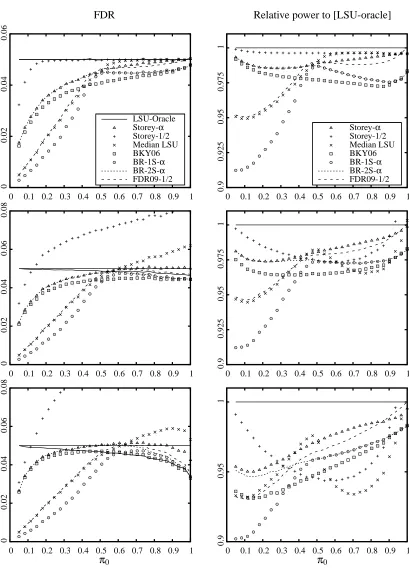
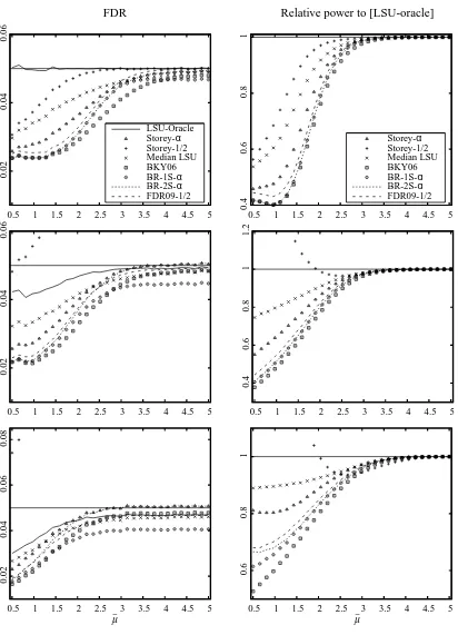
The three most important parameters in the simulation are the correlation coefficient ρ, the proportion of true null hypotheses π0, and the alternative mean ¯µ which represents the signal-to-noise ratio, or how easy it is to distinguish alternative hypotheses. We present in Figures 2, 3, and 4 results of the simulations for one varying parameter (π0, ¯µ and ρ, respectively), the others being kept fixed. Reported are, for the different methods: the FDR, and the power relative to the reference [LSU-Oracle]. Remember the absolute power is defined as the mean proportion of false null hypotheses that are correctly rejected; for each procedure the relative power is the ratio of its absolute power to that of [LSU-Oracle]. Each point is estimated by an average of 105simulations, with fixed parameters m=100 andα=5% .
3.4.1 UNDERINDEPENDENCE(ρ=0)
Remember that under independence of the p-values, the procedure [LSU] has a FDR equal toαπ0 and that the procedure [LSU Oracle] has a FDR equal to α (provided that α≤π0). The other procedures have their FDR upper bounded byα (in an asymptotical sense only for [FDR09-12]).
The situation where the p-values are independent corresponds to the first row of Figures 2 and 3 and the leftmost point of each graph in Figure 4. It appears that in the independent case, the following procedures can be consistently ordered in terms of (relative) power over the range of parameters studied here:
[Storey-12]≻[Storey-α]≻[BR08-2S-α]≻[BKY06-α], the symbol “≻” meaning “is (uniformly over our experiments) more powerful than”.
Next, the procedures [median-LSU] and [FDR09-12] appear both consistently less powerful than [Storey-12], and [FDR09-12] is additionally also consistently less powerful than [Storey-α]. Their re-lation to the remaining procedures depends on the parameters; both [median-LSU] and [FDR09-12] appear to be more powerful than the remaining procedures whenπ0>12, and less efficient other-wise. We note that [median-LSU] also appears to perform better when ¯µ is low (i.e., the alternative hypotheses are harder to distinguish).
The fact that [Storey-12] is uniformly more powerful than the other procedures in the independent case corroborates the simulations reported in Benjamini et al. (2006). Generally speaking, under independence we obtain a less biased estimate forπ−01when considering Storey’s estimator based on a “high” threshold likeλ=1
2. Namely, higher p-values are less likely to be “contaminated” by false null hypotheses; conversely, if we take a lower thresholdλ, there will be more false null hypotheses included in the set of p-values larger thanλ, leading to a pessimistic bias in the estimation ofπ−01. This qualitative reasoning is also consistent with the observed behavior of [median-LSU], since the set of p-values larger than the median is much more likely to be “contaminated” whenπ0<12.
However, the problem with [Storey-12] is that the corresponding estimation ofπ−01exhibits much more variability than its competitors when there is a substantial correlation between the p-values. As a consequence it is a very fragile procedure. This phenomenon was already pinpointed in Benjamini et al. (2006) and we study it next.
3.4.2 UNDERPOSITIVEDEPENDENCE(ρ>0)
Under positive dependence, remember that it is known theoretically from Benjamini and Yekutieli (2001) that the FDR of the procedure [LSU] (resp. [LSU Oracle]) is still bounded byαπ0(resp.α), but without equality in general. However, we do not know from a theoretical point of view if the adaptive procedures have their FDR upper bounded byα. In fact, it was pointed out by Farcomeni (2007), in another work reporting simulations on adaptive procedures, that one crucial point to this respect seems to be the variability of estimate ofπ−01. Estimates of this quantity that are not robust with respect to positive dependence will result in failures for the corresponding multiple testing procedure.
The situation where the p-values are positively dependent corresponds to the second and third rows (ρ=0.2,0.5 , respectively) of Figures 2 and 3 and to all the graphs of Figure 4 (except the leftmost points corresponding toρ=0).
FDR Relative power to [LSU-oracle]
0
0.02
0.04
0.06
0 0.1 0.2 0.3 0.4 0.5 0.6 0.7 0.8 0.9 1
LSU-Oracle Storey-α Storey-1/2 Median LSU BKY06
BR-1S-α
BR-2S-α
FDR09-1/2
0.9
0.925
0.95
0.975
1
0 0.1 0.2 0.3 0.4 0.5 0.6 0.7 0.8 0.9 1
Storey-α Storey-1/2 Median LSU BKY06
BR-1S-α
BR-2S-α
FDR09-1/2
0
0.02
0.04
0.06
0.08
0 0.1 0.2 0.3 0.4 0.5 0.6 0.7 0.8 0.9 1 0.9
0.925
0.95
0.975
1
0 0.1 0.2 0.3 0.4 0.5 0.6 0.7 0.8 0.9 1
0
0.02
0.04
0.06
0.08
0 0.1 0.2 0.3 0.4 0.5 0.6 0.7 0.8 0.9 1 0.9
0.95
1
0 0.1 0.2 0.3 0.4 0.5 0.6 0.7 0.8 0.9 1
π0 π0
FDR Relative power to [LSU-oracle]
0.02
0.04
0.06
0.5 1 1.5 2 2.5 3 3.5 4 4.5 5
LSU-Oracle Storey-α Storey-1/2 Median LSU BKY06
BR-1S-α
BR-2S-α
FDR09-1/2
0.4
0.6
0.8
1
0.5 1 1.5 2 2.5 3 3.5 4 4.5 5
Storey-α Storey-1/2 Median LSU BKY06
BR-1S-α
BR-2S-α
FDR09-1/2
0.02
0.04
0.06
0.5 1 1.5 2 2.5 3 3.5 4 4.5 5
0.4
0.6
0.8
1
1.2
0.5 1 1.5 2 2.5 3 3.5 4 4.5 5
0.02
0.04
0.06
0.08
0.5 1 1.5 2 2.5 3 3.5 4 4.5 5
0.6
0.8
1
0.5 1 1.5 2 2.5 3 3.5 4 4.5 5
¯µ ¯µ
Figure 3: FDR and power relative to oracle as a function of the common alternative hypothesis mean ¯µ . Target FDR isα=5% , total number of hypotheses m=100 . The proportion of true null hypotheses isπ0=0.5. From top to bottom: pairwise correlation coefficient
FDR Relative power to [LSU-oracle]
0
0.02
0.04
0.06
0.08
0.1
0 0.2 0.4 0.6 0.8 1 0.85
0.9
0.95
1
0 0.2 0.4 0.6 0.8 1
0.02
0.04
0.06
0.08
0 0.2 0.4 0.6 0.8 1
LSU-Oracle Storey-α Storey-1/2 Median LSU BKY06
BR-1S-α
BR-2S-α
FDR09-1/2
0.85
0.9
0.95
1
0 0.2 0.4 0.6 0.8 1
Storey-α Storey-1/2 Median LSU BKY06
BR-1S-α
BR-2S-α
FDR09-1/2
0.02
0.04
0.06
0.08
0 0.2 0.4 0.6 0.8 1 0.85
0.9
0.95
1
0 0.2 0.4 0.6 0.8 1
ρ ρ
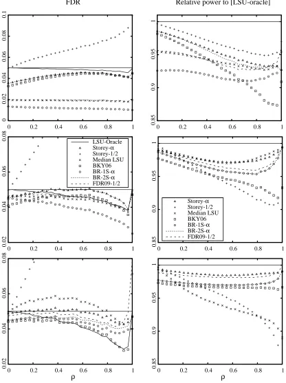
Figure 4: FDR and power relative to oracle as a function of the pairwise correlation coefficient
The other remaining procedures seem to exhibit a robust control of the FDR under dependence, or at least their FDR appears to be very close to the target level (except for [FDR09-12] whenρand
π0are close to 1). For these procedures, it seems that the qualitative conclusions concerning power comparison found in the independent case remain true. To sum up:
• the best overall procedure seems to be [Storey-α]: its FDR seems to be under or only slightly over the target level in all situations, and it exhibits globally a power superior to other proce-dures.
• then come in order of power, our two-stage procedure [BR08-2S-α], then [BKY06-α].
• like in the dependent case, [FDR09-12] ranks second whenπ0>12 but tends to perform no-ticeably poorer ifπ0 gets smaller. Its FDR is also not controlled if very strong correlations are present.
The overall conclusion we draw from these experiments is that for practical use, we recom-mend in priority [Storey-α], then as close seconds [BR08-2S-α] or [FDR09-12] (the latter when it is expected that π0>1/2 , and that there are no very strong correlations present). The procedu-dre [BKY06-α] is also competitive but appears to be in most cases noticeably outperformed by the above ones. These procedures all exhibit good robustness to dependence for FDR control as well as comparatively good power. The fact that [Storey-α] performs so well and seems to hold the favorite position has up to our knowledge not been reported before (it was not included in the simulations of Benjamini et al., 2006) and came somewhat as a surprise to us.
Remark 18 As pointed out earlier, the fact that [FDR09-12] performs sub-optimally for π0< 12
appears to be strongly linked to the choice of parameterη=12. Namely, the implicit estimator of
π−1
0 in the procedure is capped atη (see Remark 15). Choosing a higher value for ηwill reduce
the sub-optimality region but increase the variability of the estimate and thus decrease the overall robustness of the procedure (if dependence is present; and also under independence if only a small number m of hypotheses are tested, as for this procedure the convergence of the FDR towards its
asymptotically controlled value becomes slower asηgrows towards 1).
Remark 19 Another two-stage adaptive procedure was introduced in Sarkar (2008a), which is
very similar to a plug-in procedure using [Storey-λ]. In fact, in the experiments presented in Sarkar
(2008a), the two procedures are almost equivalent, corresponding toλ=0.995 . We decided not to
include this additional procedure in our simulations to avoid overloading the plots. Qualitatively, we observed that the procedures of Sarkar (2008a) or [Storey-0.995] are very similar in behavior
to [Storey-12]: very performant in the independent case but very fragile with respect to deviations
from independence.
Remark 20 One could formulate the concern that the observed FDR control for [Storey-α] could
possibly fail with other parameters settings, for example when π0 and/orρare close to one. We
performed additional simulations to this respect (a more detailed report is available on the authors’
web pages), which we summarize briefly here. We considered the following cases: π0=0.95 and
varyingρ∈[0,1];ρ=0.95 and varyingπ0∈[0,1]; finally(π0,ρ)varying both in[0.8,1]2, using a
finer discretization grid to cover this region in more detail. In all the above cases Storey-αstill had
the result of Section 3.3, stating that FDR(Storey-α) =αwhenρ=1 andπ0=1 . Finally, we also
performed additional experiments for different choices of the number of hypotheses to test (m=20
and m=104) and different choices of the target level (α=10%,1%). In all of these cases were the
results qualitatively in accordance with the ones already presented here.
4. New Adaptive Procedures with Provable FDR Control under Arbitrary Dependence
In this section, we consider from a theoretical point of view the problem of constructing multiple testing procedures that are adaptive toπ0under arbitrary dependence conditions of the p-values. The derivation of adaptive procedures that have provably controlled FDR under dependence appears to have been only studied scarcely (see Sarkar, 2008a, and Farcomeni, 2007). Here, we propose to use a two-stage procedure where the first stage is a multiple testing with either controlled FWER or controlled FDR. The first option is relatively straightfoward and is intended as a reference. In the second case, we use Markov’s inequality to estimateπ−01. Since Markov’s inequality is general but not extremely precise, the resulting procedures are obviously quite conservative and are arguably of a limited practical interest. However, we will show that they still provide an improvement, in a certain regime, with respect to the (non-adaptive) LSU procedure in the PRDS case and with respect to the family of (non-adaptive) procedures proposed in Theorem 7 in the arbitrary dependence case. For the purposes of this section, we first recall the formal definition for PRDS dependence of Benjamini and Yekutieli (2001):
Definition 21 (PRDS condition) Remember that a set D⊂[0,1]H is said to be nondecreasing if
for all x,y∈[0,1]H, if x≤y coordinate-wise, x∈D implies y∈D. Then, the p-value family p=
(ph,h∈
H
) is said to be positively regression dependent on each one fromH
0 (PRDS onH
0 inshort) if for any nondecreasing measurable set D⊂[0,1]H and for all h∈
H
0, the function u∈[0,1]7→P[p∈D|ph=u]is nondecreasing.
On the one hand, it was proved by Benjamini and Yekutieli (2001) that the LSU still has controlled FDR at levelπ0α(i.e., Theorem 6 still holds) under the PRDS assumption. On the other hand, under totally arbitrary dependence this result does not hold, and Theorem 7 provides a family of threshold collection resulting in controlled FDR at the same level in this case.
Our first result concerns a two-stage procedure where the first stage R0 is any multiple testing procedure with controlled FWER, and where we (over-) estimate m0via the straightforward estima-tor(m− |R0|). This should be considered as a form of baseline reference for this type of two-stage procedure.
Theorem 22 Let R0 be a nonincreasing multiple testing procedure and assume that its FWER is
controlled at levelα0, that is,P[R0∩
H
06=/0]≤α0. Then the adaptive step-up procedure R withdata-dependent threshold collection∆(i) =α1(m−|R0|)−1β(i)has FDR controlled at levelα0+α1
in either of the following dependence situations:
• the p-value family(ph,h∈
H
)is PRDS onH
0and the shape function is the identity function.• the p-values have unspecified dependence andβis a shape function of the form (3).
non-adaptive counterpart (using the same shape function) only if there are more than 50% rejected hypotheses in the first stage. Only if it is expected that this situation will occur does it make sense to employ this procedure, since it will otherwise perform worse than the non-adaptive procedure.
Our second result is a two-stage procedure where the first stage has controlled FDR. First intro-duce, for a fixed constantκ≥2 , the following function: for x∈[0,1],
Fκ(x) =
1 if x≤κ−1 2κ−1
1−√1−4(1−x)κ−1 otherwise
.
If R0 denotes the first stage, we propose using Fκ(|R0|/m) as an (under-)estimation of π−01 at the second stage. We obtain the following result:
Theorem 23 Let βbe a fixed shape function, and α0,α1∈(0,1) such thatα0 ≤α1. Denote by
R0 the step-up procedure with threshold collection ∆0(i) =α0β(i)/m. Then the adaptive step-up
procedure R with data-dependent threshold collection∆1(i) =α1β(i)Fκ(|R0|/m)/m has FDR upper
bounded byα1+κα0in either of the following dependence situations:
• the p-value family(ph,h∈
H
)is PRDS onH
0and the shape function is the identity function.• the p-values have unspecified dependence andβis a shape function of the form (3).
For instance, in the PRDS case, the procedure R of Theorem 23, used with κ=2, α0=α/4 andα1=α/2, corresponds to the adaptive linear step-up procedure at levelα/2 with the following estimator forπ−01:
1
1−p(2|R0|/m−1)+
,
where|R0|is the number of rejections of the LSU procedure at levelα/4.
Whether in the PRDS or arbitrary dependence case, with the above choice of parameters, we note that R is less conservative than the non-adaptive step-up procedure with threshold collection
∆(i) =αβ(i)/m if F2(|R0|/m)≥2 or equivalently when R0 rejects more than F2−1(2) =62,5% of
the null hypotheses. Conversely, R is more conservative otherwise, and we can lose up to a factor 2 in the threshold collection with respect to the standard one-stage version. Therefore, here again this adaptive procedure is only useful in the cases where it is expected that a “large” proportion of null hypotheses can easily be rejected. In particular, when we use Theorem 23 under unspecified depen-dence, it is relevant to choose the shape functionβfrom a distributionνconcentrated on the large numbers of{1, . . . ,m}. Finally, note that it is not immediate to see if this procedure will improve on the one of Theorem 22. Namely, with the above choice of parameters, procedure of Theorem 22 has the advantage of using a better estimator ofπ−01of the form(1−x)−1≥(1−p(2x−1)
+)−1in the
second round (with x=|R0|/m coming from the first round), but it has the drawback to use a first round controlling the FWER at levelα/2 which can be much more conservative than controlling the FDR at levelα/4.
To explore this issue, we performed the two above procedures, in a favorable situation whereπ0 is small. Namely, we considered the simulation setting of Section 3.4 withρ=0.1, m0=100 and