Graph Kernels
S.V. N. Vishwanathan [email protected]
Departments of Statistics and Computer Science Purdue University
250 N University Street, West Lafayette, IN 47907-2066, USA
Nicol N. Schraudolph [email protected]
adaptive tools AG
Canberra ACT 2602, Australia
Risi Kondor [email protected]
Center for the Mathematics of Information California Institute of Technology
1200 E. California Blvd., MC 305-16, Pasadena, CA 91125, USA
Karsten M. Borgwardt [email protected]
Interdepartmental Bioinformatics Group
Max Planck Institute for Developmental Biology∗ Spemannstr. 38, 72076 T¨ubingen, Germany
Editor: John Lafferty
Abstract
We present a unified framework to study graph kernels, special cases of which include the random walk (G¨artner et al.,2003;Borgwardt et al.,2005) and marginalized (Kashima et al.,2003,2004;
Mah´e et al.,2004) graph kernels. Through reduction to a Sylvester equation we improve the time complexity of kernel computation between unlabeled graphs with n vertices from O(n6)to O(n3). We find a spectral decomposition approach even more efficient when computing entire kernel ma-trices. For labeled graphs we develop conjugate gradient and fixed-point methods that take O(dn3)
time per iteration, where d is the size of the label set. By extending the necessary linear algebra to Reproducing Kernel Hilbert Spaces (RKHS) we obtain the same result for d-dimensional edge ker-nels, and O(n4)in the infinite-dimensional case; on sparse graphs these algorithms only take O(n2)
time per iteration in all cases. Experiments on graphs from bioinformatics and other application domains show that these techniques can speed up computation of the kernel by an order of mag-nitude or more. We also show that certain rational kernels (Cortes et al.,2002,2003,2004) when specialized to graphs reduce to our random walk graph kernel. Finally, we relate our framework to R-convolution kernels (Haussler,1999) and provide a kernel that is close to the optimal assignment kernel ofFr¨ohlich et al.(2006) yet provably positive semi-definite.
Keywords: linear algebra in RKHS, Sylvester equations, spectral decomposition, bioinformatics,
rational kernels, transducers, semirings, random walks
1. Introduction
Machine learning in domains such as bioinformatics (Sharan and Ideker,2006), chemoinformatics
(Bonchev and Rouvray, 1991), drug discovery (Kubinyi, 2003), web data mining
−→
Figure 1: Left: Structure of E. coli protein fragment APO-BCCP87 (Yao et al., 1997), ID 1a6x
in the Protein Data Bank (Berman et al., 2000). Right: Borgwardt et al.’s (2005) graph representation for this protein fragment. Nodes represent secondary structure elements, and edges encode neighborhood along the amino acid chain (solid) resp. in Euclidean 3D space (dashed).
(Washio and Motoda,2003), and social networks (Kumar et al., 2006) involves the study of rela-tionships between structured objects. Graphs are natural data structures to model such structures, with nodes representing objects and edges the relations between them. In this context, one often encounters two questions: “How similar are two nodes in a given graph?” and “How similar are two graphs to each other?”
In protein function prediction, for instance, one might want to predict whether a given protein is an enzyme or not. Computational approaches infer protein function by finding proteins with similar sequence, structure, or chemical properties. A very successful recent method is to model the protein as a graph (see Figure1), and assign similar functions to similar graphs (Borgwardt et al., 2005).
In Section5.2 we compute graph kernels to measure the similarity between proteins and enzymes
represented in this fashion.
Another application featured in Section5.2involves predicting the toxicity of chemical molecules by comparing their three-dimensional structure. Here the molecular structure is modeled as a graph, and the challenge is to compute the similarity between molecules of known and unknown toxicity.
Finally, consider the task of finding web pages with related content. Since documents on the web link to each other, one can model each web page as the node of a graph, and each link as an edge. Now the problem becomes that of computing similarities between the nodes of a graph. Taking this one step further, detecting mirrored sets of web pages requires computing the similarity between the graphs representing them.
Kernel methods (Sch¨olkopf and Smola, 2002) offer a natural framework to study these
ques-tions. Roughly speaking, a kernel k(x,x′) is a measure of similarity between objects x and x′. It must satisfy two mathematical requirements: it must be symmetric, that is, k(x,x′) =k(x′,x), and positive semi-definite (p.s.d.). Comparing nodes in a graph involves constructing a kernel between nodes, while comparing graphs involves constructing a kernel between graphs. In both cases, the challenge is to define a kernel that captures the semantics inherent in the graph structure and is reasonably efficient to evaluate.
The idea of constructing kernels on graphs (i.e., between the nodes of a single graph) was
con-trast, in this paper we focus on kernels between graphs. The first such kernels were proposed by G¨artner et al. (2003) and later extended byBorgwardt et al. (2005). Much at the same time, the idea of marginalized kernels (Tsuda et al.,2002) was extended to graphs by Kashima et al.(2003, 2004), then further refined byMah´e et al.(2004). Another algebraic approach to graph kernels has appeared recently (Kondor and Borgwardt,2008). A seemingly independent line of research inves-tigates the so-called rational kernels, which are kernels between finite state automata based on the algebra of abstract semirings (Cortes et al.,2002,2003,2004).
The aim of this paper is twofold: on the one hand we present theoretical results showing that all the above graph kernels are in fact closely related, on the other hand we present new algorithms for efficiently computing such kernels. We begin by establishing some notation and reviewing pertinent concepts from linear algebra and graph theory.
1.1 Paper Outline
The first part of this paper (Sections 2–5) elaborates and updates a conference publication of
Vishwanathan et al.(2007) to present a unifying framework for graph kernels encompassing many known kernels as special cases, and to discuss connections to yet others. After defining some basic concepts in Section 2, we describe the framework in Section 3, prove that it leads to p.s.d. ker-nels, and discuss the random walk and marginalized graph kernels as special cases. For ease of exposition we will work with real matrices in the main body of the paper and relegate the RKHS
extensions to AppendixA. In Section4 we present four efficient ways to compute random walk
graph kernels, namely: 1. via reduction to a Sylvester equation, 2. with a conjugate gradient solver, 3. using fixed-point iterations, and 4. via spectral decompositions. Experiments on a variety of real and synthetic data sets in Section5illustrate the computational advantages of our methods, which generally reduce the time complexity of kernel computation from O(n6)to O(n3). The experiments of Section5.3were previously presented at a bioinformatics symposium (Borgwardt et al.,2007).
The second part of the paper (Sections 6–7) draws further connections to existing kernels on structured objects. In Section6we present a simple proof that rational kernels (Cortes et al.,2002, 2003,2004) are p.s.d., and show that specializing them to graphs yields random walk graph kernels. In Section7 we discuss the relation between R-convolution kernels (Haussler, 1999) and various graph kernels, all of which can in fact be shown to be instances of R-convolution kernels. Extend-ing the framework through the use of semirExtend-ings does not always result in a p.s.d. kernel though; a case in point is the optimal assignment kernel of Fr¨ohlich et al.(2006). We establish sufficient conditions for R-convolution kernels in semirings to be p.s.d., and provide a “mostly optimal as-signment kernel” that is provably p.s.d. We conclude in Section8with an outlook and discussion.
2. Preliminaries
Here we define the basic concepts and notation from linear algebra and graph theory that will be used in the remainder of the paper.
2.1 Linear Algebra Concepts
denote the identity matrix. When it is clear from the context we will not mention the dimensions of these vectors and matrices.
Definition 1 Given real matrices A∈Rn×mand B∈Rp×q, the Kronecker product A⊗B∈Rnp×mq
and column-stacking operator vec(A)∈Rnmare defined as
A⊗B :=
A11B A12B . . . A1mB
..
. ... ... ... An1B An2B . . . AnmB
, vec(A):=
A∗1
.. . A∗m
,
where A∗j denotes the jthcolumn of A.
The Kronecker product and vec operator are linked by the well-known property (e.g.,Bernstein,
2005, Proposition 7.1.9):
vec(ABC) = (C⊤⊗A)vec(B). (1)
Another well-known property of the Kronecker product which we make use of is (Bernstein,2005,
Proposition 7.1.6):
(A⊗B)(C⊗D) =AC⊗BD. (2)
Finally, the Hadamard product of two real matrices A,B∈Rn×m, denoted by A⊙B∈Rn×m, is obtained by element-wise multiplication. It interacts with the Kronecker product via
(A⊗B)⊙(C⊗D) = (A⊙C)⊗(B⊙D). (3)
All the above concepts can be extended to a Reproducing Kernel Hilbert Space (RKHS) (See Ap-pendixAfor details).
2.2 Graph Concepts
A graph G consists of an ordered set of n vertices V ={v1,v2, . . . ,vn}, and a set of directed edges
E⊂V×V . A vertex viis said to be a neighbor of another vertex vj if they are connected by an edge, that is, if(vi,vj)∈E; this is also denoted vi∼vj. We do not allow self-loops, that is,(vi,vi)∈/E for any i. A walk of length k on G is a sequence of indices i0,i1, . . .ik such that vir−1 ∼vir for all
1≤r≤k. A graph is said to be strongly connected if any two pairs of vertices can be connected
by a walk. In this paper we will always work with strongly connected graphs. A graph is said to be undirected if(vi,vj)∈E ⇐⇒ (vj,vi)∈E.
In much of the following we will be dealing with weighted graphs, which are a slight gener-alization of the above. In a weighted graph, each edge (vi,vj) has an associated weight wi j >0 signifying its “strength”. If vi and vj are not neighbors, then wi j =0. In an undirected weighted graph wi j=wji.
When G is unweighted, we define its adjacency matrix as the n×n matrixA withe Ai je =1 if
The adjacency matrix has a normalized cousin, defined A :=A De −1, which has the property that each of its columns sums to one, and it can therefore serve as the transition matrix for a stochastic process. Here, D is a diagonal matrix of node degrees, that is, Dii=di=∑jAei j. A random walk on
G is a process generating sequences of vertices vi1,vi2,vi3, . . .according toP(ik+1|i1, . . .ik) =Aik+1,ik,
that is, the probability at vik of picking vik+1 next is proportional to the weight of the edge(vik,vik+1).
The tth power of A thus describes t-length walks, that is, (At)i j is the probability of a transition from vertex vj to vertex vi via a walk of length t. If p0 is an initial probability distribution over vertices, then the probability distribution pt describing the location of our random walker at time t is pt =Atp0. The jthcomponent of pt denotes the probability of finishing a t-length walk at vertex
vj.
A random walk need not continue indefinitely; to model this, we associate every node vik in
the graph with a stopping probability qik. Our generalized random walk graph kernels then use
the overall probability of stopping after t steps, given by q⊤pt. Like p0, the vector q of stopping probabilities is a place to embed prior knowledge into the kernel design. Since pt as a probability distribution sums to one, a uniform vector q (as might be chosen in the absence of prior knowledge) would yield the same overall stopping probability for all pt, thus leading to a kernel that is invariant with respect to the graph structure it is meant to measure. In this case, the unnormalized adjacency matrixA (which simply counts random walks instead of measuring their probability) should be usede instead.
Let
X
be a set of labels which includes the special label ζ. Every edge-labeled graph G isassociated with a label matrix X ∈
X
n×n in which Xi j is the label of the edge (vj,vi) and Xi j =ζif(vj,vi)∈/E. Let
H
be the RKHS induced by a p.s.d. kernelκ:X
×X
→R, and letφ:X
→H
denote the corresponding feature map, which we assume mapsζto the zero element of
H
. We useΦ(X)to denote the feature matrix of G (see AppendixAfor details). For ease of exposition we do not consider labels on vertices here, though our results hold for that case as well. Henceforth we use the term labeled graph to denote an edge-labeled graph.
Two graphs G= (V,E) and G′ = (V′,E′) are isomorphic (denoted by G∼=G′) if there ex-ists a bijective mapping g : V →V′ (called the isomorphism function) such that (vi,vj) ∈E iff (g(vi),g(vj))∈E′.
3. Random Walk Graph Kernels
Our generalized random walk graph kernels are based on a simple idea: given a pair of graphs, perform random walks on both, and count the number of matching walks. We show that this simple concept underlies both random walk and marginalized graph kernels. In order to do this, we first need to introduce direct product graphs.
3.1 Direct Product Graphs
Given two graphs G(V,E)and G′(V′,E′), their direct product G×is a graph with vertex set
V× ={(vi,v′r): vi∈V, v′r∈V′}, (4)
and edge set
Figure 2: Two graphs (top left & right) and their direct product (bottom). Each node of the direct product graph is labeled with a pair of nodes (4); an edge exists in the direct product if and only if the corresponding nodes are adjacent in both original graphs (5). For instance, nodes 11′and 32′are adjacent because there is an edge between nodes 1 and 3 in the first, and 1′and 2′in the second graph.
In other words, G× is a graph over pairs of vertices from G and G′, and two vertices in G× are neighbors if and only if the corresponding vertices in G and G′are both neighbors; see Figure2for an illustration. IfA ande Ae′ are the respective adjacency matrices of G and G′, then the adjacency matrix of G×isAe×=Ae⊗Ae
′
. Similarly, A×=A⊗A′.
Performing a random walk on the direct product graph is equivalent to performing a simulta-neous random walk on G and G′ (Imrich and Klavˇzar,2000). If p and p′denote initial probability distributions over the vertices of G and G′, then the corresponding initial probability distribution on the direct product graph is p×:=p⊗p′. Likewise, if q and q′are stopping probabilities (that is, the probability that a random walk ends at a given vertex), then the stopping probability on the direct product graph is q×:=q⊗q′.
Let |V|=: n and|V′|=: n′. If G and G′ are edge-labeled, we can associate a weight matrix
W× ∈Rnn
′×nn′
with G× using our extension of the Kronecker product (Definition 1) into RKHS
(Definition11in AppendixA):
As a consequence of the definition of Φ(X) and Φ(X′), the entries of W× are non-zero only if the corresponding edge exists in the direct product graph. If we simply let
H
=R,Φ(X) =A, andeΦ(X′) =Ae′then (6) reduces toAe×, the adjacency matrix of the direct product graph. Normalization can be incorporated by lettingφ(Xi j) =1/di if(vj,vi)∈E, and zero otherwise.1 ThenΦ(X) =A andΦ(X′) =A′, and consequently W×=A×.
If the edges of our graphs take on labels from a finite set, without loss of generality{1,2, . . . ,d}, we can let
H
be Rd endowed with the usual inner product. For each edge (vj,vi)∈E we setφ(Xi j) =el/di if the edge (vj,vi) is labeled l; all other entries of Φ(X) are 0. Thus the weight matrix (6) has a non-zero entry iff an edge exists in the direct product graph and the corresponding edges in G and G′ have the same label. LetlA denote the normalized adjacency matrix of the graph
filtered by the label l, that is,lAi j=Ai jif Xi j=l, and zero otherwise. Some simple algebra (omitted for the sake of brevity) shows that the weight matrix of the direct product graph can then be written as
W×= d
∑
l=1
lA⊗lA′. (7)
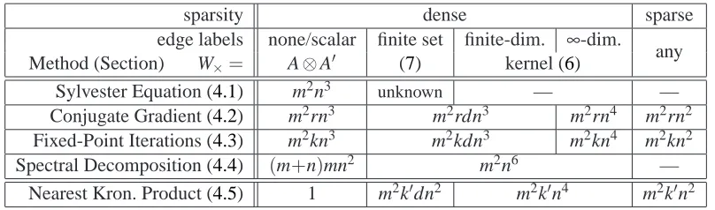
In Section4we will develop efficient methods to compute kernels defined using the weight matrix of the direct product graph. The applicability and time complexity of a particular method will depend on whether the graphs are unlabeled though possibly edge-weighted (W×=A×), have discrete edge
labels (7), or—in the most general case—employ an arbitrary edge kernel (6); see Table 1 for a
summary.
3.2 Kernel Definition
As stated above, performing a random walk on the direct product graph G× is equivalent to
per-forming a simultaneous random walk on the graphs G and G′ (Imrich and Klavˇzar,2000).
There-fore, the((i−1)n′+r,(j−1)n′+s)th entry of Ak
×represents the probability of simultaneous length
k random walks on G (starting from vertex vj and ending in vertex vi) and G′ (starting from ver-tex v′s and ending in vertex v′r). The entries of W× (6) represent similarity between edges: The ((i−1)n′+r,(j−1)n′+s) entry of W×k represents the similarity between simultaneous length k random walks on G and G′, measured via the kernel functionκ. Given initial and stopping proba-bility distributions p×and q×one can compute q⊤×W×kp×, which is the expected similarity between simultaneous length k random walks on G and G′.
To define a kernel which computes the similarity between G and G′, one natural idea is to simply sum up q⊤×W×kp×for all values of k. However, this sum might not converge, leaving the kernel value undefined. To overcome this problem, we introduce appropriately chosen non-negative coefficients
µ(k), and define the kernel between G and G′as
k(G,G′):=
∞
∑
k=0
µ(k)q⊤×W×kp×. (8)
This definition is very flexible and offers the kernel designer many parameters to adjust in an application-specific manner: Appropriately choosing µ(k) allows one to (de-)emphasize walks of different lengths; if initial and stopping probabilities are known for a particular application, then
this knowledge can be incorporated into the kernel; and finally, appropriate kernels or similarity measures between edges can be incorporated via the weight matrix W×. Despite its flexibility, this kernel is guaranteed to be p.s.d. and—as we will see in Section4—can be computed efficiently by exploiting the special structure of W×. To show that (8) is a valid p.s.d. kernel we need the following technical lemma:
Lemma 2 ∀k∈N: W×kp×=vec[Φ(X′)kp′(Φ(X)kp)⊤]. Proof By induction over k. Base case: k=0. Using (1) we find
W×0p×=p×= (p⊗p′)vec(1) =vec(p′1 p⊤) =vec[Φ(X′)0p′(Φ(X)0p)⊤]. (9) Induction from k to k+1: Using the induction assumption W×kp×=vec[Φ(X′)kp′(Φ(X)kp)⊤]and
Lemma12we obtain
W×k+1p×=W×W×kp×= (Φ(X)⊗Φ(X′))vec[Φ(X′)kp′(Φ(X)kp)⊤]
=vec[Φ(X′)Φ(X′)kp′(Φ(X)kp)⊤Φ(X)⊤] (10) =vec[Φ(X′)k+1p′(Φ(X)k+1p)⊤].
Base case (9) and induction (10) together imply Lemma2∀k∈N0.
Theorem 3 If the coefficients µ(k)are such that (8) converges, then (8) defines a valid p.s.d. kernel.
Proof Using Lemmas12and2we can write
q⊤×W×kp×= (q⊗q′)⊤vec[Φ(X′)kp′(Φ(X)kp)⊤] =vec[q′⊤Φ(X′)kp′(Φ(X)kp)⊤q] = (q⊤Φ(X)kp)⊤
| {z }
ρk(G)⊤
(q′⊤Φ(X′)kp′)
| {z }
ρk(G′)
. (11)
Each individual term of (11) equals ρk(G)⊤ρk(G′) for some function ρk, and is therefore a valid p.s.d. kernel. The theorem follows because the class of p.s.d. kernels is closed under non-negative linear combinations and pointwise limits (Berg et al.,1984).
3.3 Special Cases
Kashima et al.(2004) define a kernel between labeled graphs via walks and their label sequences. Recall that a walk of length t on G is a sequence of indices i1,i2, . . .it+1such that vik ∼vik+1 for all
and q denote starting and stopping probabilities. Then one can compute the probability of a walk
i1,i2, . . .it+1and hence the label sequence h associated with it as
p(h|G):=qit+1
t
∏
j=1
Pij,ij+1pi1. (12)
Now let ˆφ denote a feature map on edge labels, and define a kernel between label sequences of length t by
κ(h,h′):= t
∏
i=1
κ(hi,h′i) = t
∏
i=1 ˆ
φ(hi),φˆ(h′i)
(13)
if h and h′have the same length t, and zero otherwise. Using (12) and (13) we can define a kernel between graphs via marginalization:
k(G,G′):=
∑
h∑
h′κ(h,h′)p(h|G)p(h|G′). (14)
Kashima et al.(2004, Eq. 1.19) show that (14) can be written as
k(G,G′) =q⊤×(I−T×)−1p×, (15) where T×= [vec(P)vec(P′)⊤]⊙[Φˆ(X)⊗Φˆ(X′)]. (As usual, X and X′denote the edge label matrices of G and G′, respectively, and ˆΦthe corresponding feature matrices.)
Although this kernel is differently motivated, it can be obtained as a special case of our frame-work. Towards this end, assume µ(k) =λk for someλ>0. We can then write
k(G,G′) =
∞
∑
k=0
λkq⊤
×W×kp× = q⊤×(I−λW×)−1p×. (16) To recover the marginalized graph kernels letλ=1, and defineΦ(Xi j) =Pi jΦˆ(Xi j), in which case
W×=T×, thus recovering (15).
Given a pair of graphs,G¨artner et al.(2003) also perform random walks on both, but then count the number of matching walks. Their kernel is defined as (G¨artner et al.,2003, Definition 6):
k(G,G′) = n
∑
i=1 n′
∑
j=1
∞
∑
k=0
λk h
e A×k
i
i j. (17) To obtain (17) in our framework, set µ(k):=λk, assume uniform distributions for the starting and stopping probabilities over the vertices of G and G′(i.e., pi=qi=1/n and pi′=q′i=1/n′), and let
Φ(X):=A ande Φ(X′) =Ae′. Consequently, p×=q×=e/(nn′), and W×=Ae×, the unnormalized adjacency matrix of the direct product graph. This allows us to rewrite (8) to obtain
k(G,G′) =
∞
∑
k=0
µ(k)q⊤×W×kp× = 1
n2n′2 n
∑
i=1 n′
∑
j=1
∞
∑
k=0
λk h
e A×k
i
sparsity dense sparse
edge labels none/scalar finite set finite-dim. ∞-dim.
any
Method (Section) W×= A⊗A′ (7) kernel (6)
Sylvester Equation (4.1) m2n3 unknown — —
Conjugate Gradient (4.2) m2rn3 m2rdn3 m2rn4 m2rn2
Fixed-Point Iterations (4.3) m2kn3 m2kdn3 m2kn4 m2kn2
Spectral Decomposition (4.4) (m+n)mn2 m2n6 —
Nearest Kron. Product (4.5) 1 m2k′dn2 m2k′n4 m2k′n2
Table 1: Worst-case time complexity (in O(·)notation) of our methods for an m×m graph kernel
matrix, where n=size of the graphs (number of nodes), d=size of label set resp. dimen-sionality of feature map, r=effective rank of W×, k=number of fixed-point iterations (31), and k′=number of power iterations (37).
unnormalized) adjacency matrices, analogous to our (7). The reduction to our framework extends to this setting in a straightforward manner.
G¨artner et al.(2003) discuss two cases of special interest: First, their geometric kernel employs a fixed decay factorλto down-weight the contribution of long walks to the kernel, settingλk:=λkas in our (16). The choice ofλis critical here: It must be small enough for the sum in (17) to converge,
depending on the spectrum of W× (Vishwanathan, 2002, Chapter 6). Second, their exponential
kernel is defined as
k(G,G′) = n
∑
i=1 n′
∑
j=1 [eλAe×]
i j=e⊤eλAe×e, (19) using the matrix exponential. This is obtained in our framework by settingλk:=λk/k!, so that the right-most sum in (18) becomes the series expansion of eλAe×.
The kernels ofG¨artner et al.(2003) differ from our definition (8) in that they do not explicitly model starting or stopping probabilities, and employ unnormalized adjacency matrices instead of our more general weight matrix (6) which allows for normalization and arbitrary kernels on edges.
4. Efficient Computation
Computing a geometric random walk graph kernel with µ(k) =λkamounts to inverting(I−λW ×), an n2×n2 matrix if G and G′ have n vertices each. Since the complexity of inverting a matrix is essentially cubic in its dimensions, direct computation of (16) would require O(n6)time. Below we develop methods based on Sylvester equations (Section4.1), conjugate gradients (Section4.2), fixed-point iterations (Section4.3), and spectral decompositions (Section4.4) that greatly accelerate
this computation. Section 4.5 introduces an approximation that can further speed up the kernel
computation for labeled graphs.
Table 1 summarizes our results, listing the worst-case time complexity of our methods as a
for conjugate gradient, and by (31) for fixed-point iterations. The spectral decomposition approach (Section4.4) is exceptional here in that it can be linear in m resp. quadratic in n (but not both) if precomputation of the m spectral graph decompositions dominates (resp. is dominated by) the actual kernel computations.
The cost of the iterative algorithms increases by another factor of d for graphs with edge labels from a finite set of d symbols or an edge kernel with d-dimensional feature map; for an arbitrary edge kernel (whose feature map may be infinite-dimensional) this factor becomes n. On labeled graphs our spectral decomposition approach offers no savings, and the Sylvester equation method applies only if the labels come from a finite set of symbols, and then with unknown time complexity. A nearest Kronecker product approximation can be used, however, to approximate the direct product of labeled graphs with a weight matrix that can be handled by any of our methods for unlabeled graphs. This approximation requires k′ (37) iterations, each costing O(dn2) time when the labels come from a finite set of d symbols, and O(n4)in general.
Finally, when the graphs are sparse (i.e., only have O(n) edges each; rightmost column in Ta-ble1) our iterative methods (conjugate gradient, fixed-point, and nearest Kronecker product) take only O(n2)time per iteration, regardless of how the graphs are labeled. We cannot authoritatively state the time complexity for sparse graphs of solving Sylvester equations or performing spectral decompositions.Spielman and Teng(2008) have shown that graphs can be sparsified (i.e., approxi-mated by sparse graphs) in nearly linear time, although the constants involved are quite large.
4.1 Sylvester Equation Methods
Consider the following equation, commonly known as the Sylvester or Lyapunov equation:
M=SMT+M0. (20)
Here, S,T,M0∈Rn×nare given and we need to solve for M∈Rn×n. These equations can be readily solved in O(n3) time with freely available code (Gardiner et al., 1992), such as Matlab’s dlyap
method. Solving the generalized Sylvester equation
M= d
∑
i=1
SiMTi+M0 (21)
involves computing generalized simultaneous Schur factorizations of d symmetric matrices (Lathauwer et al., 2004). Although technically involved, (21) can also be solved efficiently, al-beit at a higher computational cost. The computational complexity of this generalized factorization is at present unknown.
We now show that for graphs with discrete edge labels, whose weight matrix W×can be written as (7), the problem of computing the graph kernel (16) can be reduced to solving the following generalized Sylvester equation:
M= d
∑
i=1
λiA′MiA⊤+M
0, (22)
where vec(M0) =p×. We begin by flattening (22): vec(M) =λ
d
∑
i=1
vec(iA′MiA⊤) +p
Using Lemma12(which extends (1) into an RKHS) we can rewrite (23) as
(I−λ d
∑
i=1
iA⊗iA′)vec(M) =p
×, (24)
use (7), and solve (24) for vec(M):
vec(M) = (I−λW×)−1p×. (25)
Multiplying both sides of (25) by q⊤×yields
q⊤×vec(M) =q⊤×(I−λW×)−1p×. (26) The right-hand side of (26) is the graph kernel (16). Given the solution M of the Sylvester equation (22), the graph kernel can be obtained as q⊤×vec(M)in O(n2) time. The same argument
applies for unlabeled graphs by simply setting d =1, which turns (22) into a simple Sylvester
equation. Since solving that only takes O(n3)time, computing the random walk graph kernel in this fashion is much faster than the O(n6)time required by the direct approach.
One drawback of this strategy is that Sylvester equation solvers are quite sophisticated and typically available only as black-box library routines, which limits their applicability. Matlab’s
dlyapsolver, for instance, does not exploit sparsity, and only handles the cases d=1 and d=2. A solver for the simple Sylvester equation (20) can still be used to efficiently compute kernels between labeled graphs though by employing the nearest Kronecker product approximation (Section4.5).
4.2 Conjugate Gradient Methods
Given a matrix M and a vector b, conjugate gradient (CG) methods solve the system of equations
Mx=b efficiently (Nocedal and Wright,1999). While they are designed for symmetric p.s.d. ma-trices, CG solvers can also be used to solve other linear systems efficiently. They are particularly efficient if the matrix is rank deficient, or has a small effective rank, that is, number of distinct eigenvalues. Furthermore, if computing matrix-vector products is cheap—because M is sparse, for instance—the CG solver can be sped up significantly (Nocedal and Wright,1999). Specifically, if computing Mv for an arbitrary vector v requires O(m)time, and the effective rank of M is r, then a CG solver takes O(r)iterations, and hence only O(rm)time, to solve Mx=b.
The graph kernel (16) can be computed by a two-step procedure: First we solve the linear system
(I−λW×)x=p×, (27)
for x, then we compute q⊤×x. We now focus on efficient ways to solve (27) with a CG solver. Recall that if G and G′ contain n vertices each then W× is an n2×n2 matrix. Naively, multiplying W by some vector y inside the CG algorithm requires O(n4)operations. However, by our extension of the vec-ABC formula (1) into RKHS (Lemma12), introducing the matrix Y ∈Rn×n with y=vec(Y), and recalling that W×=Φ(X)⊗Φ(X′), by Lemma12we can write
W×y= (Φ(X)⊗Φ(X′))vec(Y) =vec(Φ(X′)YΦ(X)⊤). (28)
Ifφ(·)∈Rd then the above matrix-vector product can be computed in O(dn3)time. If Φ(X)and
4.3 Fixed-Point Iterations
Fixed-point methods begin by rewriting (27) as
x=p×+λW×x. (29)
Now, solving for x is equivalent to finding a fixed point of (29) taken as an iteration (Nocedal and Wright,1999). Letting xt denote the value of x at iteration t, we set x0:=p×, then compute
xt+1=p×+λW×xt (30)
repeatedly untilkxt+1−xtk<ε, wherek · kdenotes the Euclidean norm and εsome pre-defined tolerance. This is guaranteed to converge if all eigenvalues ofλW×lie inside the unit disk; this can be ensured by settingλ<|ξ1|−1, where ξ1is the largest-magnitude eigenvalue of W×. Assuming that each iteration of (30) contracts x to the fixpoint by a factor ofλξ1, we converge to withinεof the fixpoint in k iterations, where
k=O
lnε lnλ+ln|ξ1|
. (31)
The above is closely related to the power method used to compute the largest eigenvalue of a matrix (Golub and Van Loan,1996); efficient preconditioners can also be used to speed up
con-vergence (Golub and Van Loan, 1996). Since each iteration of (30) involves computation of the
matrix-vector product W×xt, all speed-ups for computing the matrix-vector product discussed in Section4.2 are applicable here. In particular, we exploit the fact that W× is a sum of Kronecker products to reduce the worst-case time complexity to O(dn3)per iteration in our experiments, in contrast toKashima et al.(2004) who computed the matrix-vector product explicitly.
4.4 Spectral Decomposition Method
In the previous two sections we have introduced methods that are efficient for both unlabeled and labeled graphs, but specifically computed the geometric kernel (16), that is, assumed that µ(k) =λk. We now turn to a method based on spectral decompositions that can compute the general random walk kernel (8) for any convergent choice of µ(k), but is only efficient for unlabeled graphs. (In fact, it will turn out to be our most efficient method for computing an entire kernel matrix between unlabeled graphs.)
Let W×=P×D×P×−1denote the spectral decomposition of W×, that is, the columns of P×are its
eigenvectors, and D× is a diagonal matrix of corresponding eigenvalues. The random walk graph
kernel (8) can then be written as
k(G,G′) :=
∞
∑
k=0
µ(k)q⊤×(P×D×P×−1)kp× = q⊤×P×
∞
∑
k=0
µ(k)D×k
!
P×−1p×. (32) This simplifies matters in that (32) only takes weighted powers of a diagonal matrix, which decouple into scalar powers of its entries. An implementable graph kernel can then be obtained by employing a power series that is known to converge to a given nonlinear function. The geometric kernel (16), for instance, uses the fact that∑∞k=0xk= 1
1−x; setting µ(k):=λ
k in (32) we thus obtain
The crucial difference to (16) is that the inverse in (33) is of a diagonal matrix, hence trivial to compute: just take the reciprocal of each entry. To give another example, setting µ(k):=λk/k! in (32) yields the exponential kernel (19) by way of spectral decomposition:
k(G,G′) := q⊤×P×eλD×P×−1p×, (34) because ex=∑∞k=0xk/k!. Again, unlike in (19) the matrix exponential here is trivial to compute becauseλD×is diagonal: simply exponentiate each entry.
Thus by diagonalizing the nonlinearity central to a random walk graph kernel, spectral decom-position can greatly expedite its computation. As described above, however, it is computationally unattractive: Computing the spectral decomposition of a dense matrix takes time cubic in its size (Golub and Van Loan, 1996); since W× is an n2×n2 matrix this would result in O(n6)time com-plexity per kernel computation.2 By leveraging the properties of the Kronecker product, however, we can obtain a far better result for unlabeled (though possibly edge-weighted) graphs:
Theorem 4 The kernel matrix for any random walk kernel (8) between m unlabeled, possibly
edge-weighted graphs with n nodes can be computed in O((mp+n)mn2)time via spectral decompositions, where computing the corresponding scalar power series takes O(p)time.
Proof Because the graphs are unlabeled, we have W× :=A×=Ai⊗Aj, where Ai and Aj (i,j∈ {1,2, . . . ,m}) are the adjacency matrices (normalized or not) of individual graphs. Begin by pre-computing the spectral decomposition of each graph: (∀i)Ai=PiDiPi−1. Using Propositions 7.1.6, 7.1.7 ofBernstein(2005) we have
Ai⊗Aj = (PiDiPi−1)⊗(PjDjPj−1) = (Pi⊗Pj)(Di⊗Dj)(Pi⊗Pj)−1. (35) Proposition 7.1.10 ofBernstein(2005) tells us that in fact Di⊗Dj =D×, which implies that also
Pi⊗Pj=P× and that indeed the spectral decomposition of a Kronecker product decomposes into those of its constituents, as seen in (35). We can therefore use Propositions 7.1.6, 7.1.7 ofBernstein (2005) again to rewrite (32) as
k(Gi,Gj) = (qi⊤Pi⊗q⊤jPj)
∞
∑
k=0
µ(k)(Di⊗Dj)k !
(Pi−1pi⊗P−j 1pj). (36)
Computing the central power series here takes O(n2p)time just as in (32), but the cost of calculating the two flanking factors has been reduced from O(n4) to O(n2) in (36). The entire m×m kernel
matrix can thus be obtained in O(m2n2p)time, plus the O(mn3)time it takes to precompute spectral decompositions of the m individual adjacency matrices.
Note that in practice we will always pick a power series with known limit that is trivial to evaluate (i.e., p=1), as exemplified by the geometric (33) and exponential (34) kernels. Theorem4 then gives us a very efficient method to compute entire kernel matrices, albeit only between unlabeled graphs. (It is tempting to try to extend the spectral approach for the exponential kernel to labeled graphs, but this runs into a key technical difficulty: a sum of (label-filtered adjacency) matrices in the exponent cannot be separated unless those matrices commute, that is, generally eA+B6=eAeB
unless AB=BA.)
4.5 Nearest Kronecker Product Approximation
As we have seen above, some of our fast methods for computing random walk graph kernels may become computationally expensive, or not even be available, for labeled graphs, in particular when the number d of distinct labels is large or a general edge kernel is employed. In such cases we can find the nearest Kronecker product to W×, that is, compute matrices S and T such that W×≈S⊗T ,
then use any of our methods on S⊗T as if it were the adjacency matrix of a direct product of
unlabeled graphs.
Finding the nearest Kronecker product approximating a matrix such as W× is a well-studied
problem in numerical linear algebra, and efficient algorithms which can exploit the sparsity of W× are available (Pitsianis,1992;Van Loan,2000). Formally, these methods minimize the Frobenius normkW×−S⊗TkFby computing the largest singular value of ˆW×, a permuted version of W×. We employ the power method3 for this purpose, each iteration of which entails computing the matrix-vector product ˆW×vec(T′), where T′∈Rn×n is the current approximation of T . The result of the matrix-vector product is then reshaped into an n×n matrix to form T′for the next iteration (Pitsianis, 1992). It is easy to see that computing ˆW×vec(T′)requires O(n4)time.
If W× can be written as a sum of d Kronecker products (7), then so can ˆW× (Pitsianis, 1992; Van Loan,2000), and the cost per iteration hence drops to O(dn2). Furthermore, if the two graphs are sparse with O(n)edges each, then W×will have O(n2)non-zero entries, and each iteration only takes O(n2)time. The number k′ of iterations required is
k′=O
ln n ln|ξ1| −ln|ξ2|
, (37)
whereξ1andξ2are the eigenvalues of W×with largest resp. second-largest magnitude.
As described above, the nearest Kronecker product approximation is calculated separately for each entry of an m×m kernel matrix. This causes two problems: First, the spectral decomposition
method will now take O(m2n3)time, as it is no longer possible to precompute the m graph spec-tra. Second, like the optimal assignment kernel (Section7.2) the resulting kernel matrix may have negative eigenvalues, and hence fail to be p.s.d. In future work, it may be possible to address these shortcomings by computing a simultaneous nearest Kronecker product approximation for the entire kernel matrix. For now, we verified empirically on the MUTAG and PTC data sets (cf. Section5.2) that the most negative eigenvalue is relatively small: its magnitude was 4.4% resp. 0.1% ofξ2. We also found the nearest Kronecker product to provide a better approximation than simply ignoring the graph labels: the angle between vec(W×)and its unlabeled variant was 2.2 resp. 4.7 times greater than that between vec(W×)and vec(S⊗T).
5. Experiments
Numerous studies have applied random walk graph kernels to problems such as protein function prediction (Borgwardt et al., 2005) and chemoinformatics (Kashima et al., 2004). In our experi-ments we therefore focus on the runtime of computing the kernels, rather than their utility in any given application. We present three sets of experiments: First, we study the scaling behaviour of our algorithms on unlabeled random graphs. Second, we assess the practical impact of our algorithmic improvement on four real-world data sets whose size mandates fast kernel computation. Third, we
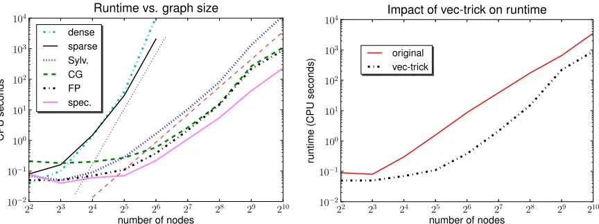
Figure 3: Time to compute a 10×10 kernel matrix on random graphs with n nodes and 3n edges as a function of the graph size n. Left: The Sylvester equation (Sylv.), conjugate gradient (CG), fixed-point iteration (FP), and spectral decomposition (spec.) approaches, com-pared to the dense and sparse direct method. Thin straight lines indicate O(n6) (black dots) resp. O(n3) (red dashes) scaling. Right: Kashima et al.’s (2004) fixed-point itera-tion (original) compared to our version, which exploits Lemma12(vec-trick).
devise novel methods for protein-protein interaction (PPI) network comparison using graph kernels. The algorithmic challenge here is to efficiently compute kernels on large sparse graphs.
The baseline for comparison in all our experiments is the direct approach of G¨artner et al. (2003), implemented via a sparse LU factorization; this already runs orders of magnitude faster on our data sets than a dense (i.e., non-sparse) implementation. Our code was written in Matlab Release 2008a, and all experiments were run under Mac OS X 10.5.5 on an Apple Mac Pro with a
3.0 GHz Intel 8-Core processor and 16 GB of main memory. We employed Lemma12to speed up
matrix-vector multiplication for both CG and fixed-point methods (cf. Section 4.2), and used the functiondlyapfrom Matlab’s control toolbox to solve the Sylvester equation. By default, we used a value ofλ=10−4, and set the convergence tolerance for both CG solver and fixed-point iteration to 10−6. For the real-world data sets, the value ofλwas chosen to ensure that the random walk graph kernel converges. Since our methods are exact and produce the same kernel values (to numerical precision), we only report the CPU time of each algorithm.
5.1 Unlabeled Random Graphs
The aim here is to study the scaling behaviour of our algorithms as a function of graph size and sparsity. We generated several sets of unlabeled random graphs. For the first set we began with an empty graph of n=2k nodes, where k=2,3, . . . ,10, randomly added 3n edges, then checked the graph’s connectivity. For each k we repeated this process until we had collected 10 strongly connected random graphs.
The time required to compute the 10×10 kernel matrix between these graphs for each value of
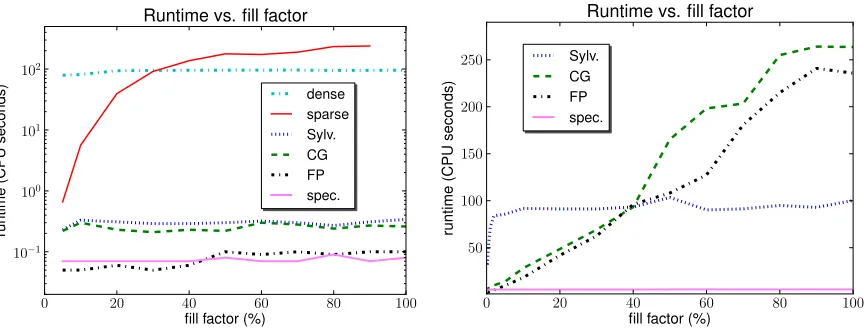
Figure 4: Time to compute a 10×10 kernel matrix on random graphs as a function of their fill factor. Left: The dense and sparse direct method on 32-node graphs, compared to our Sylvester equation (Sylv.), conjugate gradient (CG), fixed point iteration (FP), and spectral decom-position (spec.) approaches. Right: Our approaches on larger graphs with 256 nodes, where the direct method is infeasible.
conjugate gradient (CG) and fixed-point iteration (FP) methods, by contrast, all scale as O(n3), and can thus be applied to far larger graphs. Our spectral decomposition approach (spec.) is the fastest method here; it too scales as O(n3)as n asymptotically dominates over the fixed kernel matrix size
m=10.
We also examined the impact of Lemma12on enhancing the runtime performance of the
fixed-point iteration approach as originally proposed byKashima et al.(2004). For this experiment, we
again computed the 10×10 kernel matrix on the above random graphs, once using the original
fixed-point iteration, and once using fixed-point iteration enhanced by Lemma 12. As Figure 3
(right) shows, our approach consistently outperforms the original version, sometimes by over an order of magnitude.
For the next set of experiments we fixed the graph size at 32 nodes (the largest size that the direct method could handle comfortably), and randomly added edges until the fill factor (i.e., the number of non-zero entries in the adjacency matrix) reached x%, where x=5,10,20,30, . . . ,100.
For each x, we generated 10 such graphs and computed the 10×10 kernel matrix between them.
Figure4(left) shows that as expected, the sparse direct method is faster than its dense counterpart for small fill factors but slower for larger ones. Both however are consistently outperformed by our four methods, which are up to three orders of magnitude faster, with fixed-point iterations (FP) and spectral decompositions (spec.) the most efficient.
adja-cency matrices. The same holds for our spectral decomposition approach, which however exhibits impressive performance here: although it does not exploit sparsity at all, it is the fastest method by far on all but the sparsest (≤2% filled) graphs. Clearly, well-designed sparse implementations of Sylvester equation solvers, and in particular spectral decomposition, could facilitate substantial further gains in efficiency here.
5.2 Real-World Data Sets
Our next set of experiments used four real-world data sets: Two sets of molecular compounds (MUTAG and PTC), and two data sets describing protein tertiary structure (Protein and Enzyme). Graph kernels provide useful measures of similarity for all of these.
5.2.1 THEDATASETS
We now briefly describe each data set, and discuss how graph kernels are applicable.
Chemical Molecules. Toxicity of chemical molecules can be predicted to some degree by
compar-ing their three-dimensional structure. We employed graph kernels to measure similarity between
molecules from the MUTAG and PTC data sets (Toivonen et al., 2003). The average number of
nodes per graph in these data sets is 17.72 resp. 26.70; the average number of edges is 38.76 resp. 52.06.
Protein Graphs. A standard approach to protein function prediction involves classifying proteins
into enzymes and non-enzymes, then further assigning enzymes to one of the six top-level classes
of the Enzyme Commission (EC) hierarchy. Towards this end, Borgwardt et al.(2005) modeled a
data set of 1128 proteins as graphs in which vertices represent secondary structure elements, and edges represent neighborhood within the 3-D structure or along the amino acid chain, as illustrated in Figure1.
Comparing these graphs via a modified random walk graph kernel and classifying them with a Support Vector Machine (SVM) led to function prediction accuracies competitive with state-of-the-art approaches (Borgwardt et al.,2005). We usedBorgwardt et al.’s (2005) data to test the efficacy of our methods on a large data set. The average number of nodes and edges per graph in this data is 38.57 resp. 143.75. We used a single label on the edges, and the delta kernel to define similarity between edges.
Enzyme Graphs. We repeated the above experiment on an enzyme graph data set, also due to
Borgwardt et al.(2005). This data set contains 600 graphs, with 32.63 nodes and 124.27 edges on
average. Graphs in this data set represent enzymes from the BRENDA enzyme database
(Schomburg et al.,2004). The biological challenge on this data is to correctly assign the enzymes to one of the EC top-level classes.
5.2.2 UNLABELEDGRAPHS
For this experiment, we computed kernels taking into account only the topology of the graph, that is, we did not consider node or edge labels. Table2lists the CPU time required to compute the full
kernel matrix for each data set, as well as—for comparison purposes—a 100×100 submatrix. The
data set MUTAG PTC Enzyme Protein
nodes/graph 17.7 26.7 32.6 38.6
edges/node 2.2 1.9 3.8 3.7
#graphs 100 230 100 417 100 600 100 1128
Sparse 31” 1’45” 45” 7’23” 1’52” 1h21’ 23’23” 2.1d*
Sylvester 10” 54” 28” 7’33” 31” 23’28” 5’25” 11h29’
Conj. Grad. 23” 1’29” 26” 4’29” 14” 10’00” 45” 39’39”
Fixed-Point 8” 43” 15” 2’38” 5” 5’44” 43” 22’09”
Spectral 5” 27” 7” 1’54” 7” 4’32” 27” 23’52”
∗extrapolated number of days; run did not finish in time available.
Table 2: Time to compute kernel matrix for unlabeled graphs from various data sets.
On these unlabeled graphs, conjugate gradient, fixed-point iterations, and spectral
decompositions—sped up via Lemma 12—are consistently faster than the sparse direct method.
The Sylvester equation approach is very competitive on smaller graphs (outperforming CG on MU-TAG) but slows down with increasing number of nodes per graph. Even so, it still outperforms the sparse direct method. Overall, spectral decomposition is the most efficient approach, followed by fixed-point iterations.
5.2.3 LABELEDGRAPHS
For this experiment, we compared graphs with edge labels. Note that node labels can be dealt with by concatenating them to the edge labels of adjacent edges. On the two protein data sets we employed a linear kernel to measure similarity between edge weights representing distances (in
˚
Angstr¨oms) between secondary structure elements; since d=1 we can use all our methods for
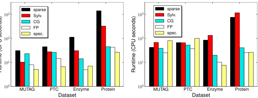
unlabeled graphs here. On the two chemical data sets we used a delta kernel to compare edge labels reflecting types of bonds in molecules; for the Sylvester equation and spectral decomposition approaches we then employed the nearest Kronecker product approximation. We report CPU times for the full kernel matrix as well as a 100×100 submatrix in Table 3; the latter is also shown graphically in Figure5(right).
On labeled graphs, the conjugate gradient and the fixed-point iteration always outperform the sparse direct approach, more so on the larger graphs and with the linear kernel. As expected, spectral decompositions are inefficient in combination with the nearest Kronecker product approximation,
kernel delta, d=7 delta, d=22 linear, d=1
data set MUTAG PTC Enzyme Protein
#graphs 100 230 100 417 100 600 100 1128
Sparse 42” 2’44” 1’07” 14’22” 1’25” 57’43” 12’38” 1.1d*
Sylvester 1’08” 6’05” 1’06” 18’20” 2’13” 76’43” 19’20” 11h19’
Conj. Grad. 39” 3’16” 53” 14’19” 20” 13’20” 41” 57’35”
Fixed-Point 25” 2’17” 37” 7’55” 10” 6’46” 25” 31’09”
Spectral 1’20” 7’08” 1’40” 26’54” 8” 4’22” 26” 21’23”
∗extrapolated number of days; run did not finish in time available.
Figure 5: Time (in seconds on a log-scale) to compute 100×100 kernel matrix for unlabeled (left)
resp. labeled (right) graphs from several data sets, comparing the conventional sparse
method to our fast Sylvester equation, conjugate gradient (CG), fixed-point iteration (FP), and spectral approaches.
but with the linear kernel they perform as well as fixed-point iterations for m=100, and better yet on the large kernel matrices. The Sylvester equation approach (at least with the Sylvester solver we used) cannot take advantage of sparsity, but still manages to perform almost as well as the sparse direct method.
5.3 Protein-Protein Interaction Networks
In our third experiment, we used random walk graph kernels to tackle a large-scale problem in bioinformatics involving the comparison of fairly large protein-protein interaction (PPI) networks. Using a combination of human PPI and clinical microarray gene expression data, the task is to predict the disease outcome (dead or alive, relapse or no relapse) of cancer patients. As before, we setλ=0.001 and the convergence tolerance to 10−6for all our experiments reported below.
5.3.1 CO-INTEGRATION OFGENEEXPRESSION ANDPPI DATA
We co-integrated clinical microarray gene expression data for cancer patients with known human PPI fromRual et al.(2005). Specifically, a patient’s gene expression profile was transformed into a
graph as follows: A node was created for every protein which—according toRual et al.(2005)—
participates in an interaction, and whose corresponding gene expression level was measured on this patient’s microarray. We connect two proteins in this graph by an edge if Rual et al. (2005) list these proteins as interacting, and both genes are up- resp. downregulated with respect to a reference measurement. Each node bears the name of the corresponding protein as its label.
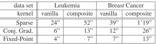
data set Leukemia Breast Cancer
kernel vanilla composite vanilla composite
Sparse 24” 52” 39” 1’19”
Conj. Grad. 6” 13” 12” 26”
Fixed-Point 4” 7” 7” 13”
Table 4: Average time to compute kernel matrix on protein-protein interaction networks.
natural choice, as a random walk in this graph represents a group of proteins in which consecutive proteins along the walk are co-expressed and interact. As each node bears the name of its corre-sponding protein as its node label, the size of the product graph is at most that of the smaller of the two input graphs.
5.3.2 COMPOSITEGRAPHKERNEL
The presence of an edge in a graph signifies an interaction between the corresponding nodes. In chemoinformatics, for instance, edges indicate chemical bonds between two atoms; in PPI net-works, edges indicate interactions between proteins. When studying protein interactions in disease, however, the absence of a given interaction can be as significant as its presence. Since existing graph kernels cannot take this into account, we propose to modify them appropriately. Key to our approach is the notion of a complement graph:
Definition 5 Let G= (V,E)be a graph with vertex set V and edge set E. Its complement ¯G= (V,E¯)
is a graph over the same vertices but with complementary edges ¯E := (V×V)\E.
In other words, the complement graph consists of exactly those edges not present in the original graph. Using this notion we define the composite graph kernel
kcomp(G,G′):=k(G,G′) +k(G¯,G¯′). (38) This deceptively simple kernel leads to substantial gains in performance in our experiments com-paring co-integrated gene expression/protein-protein interaction networks.
5.3.3 DATASETS
Leukemia.Bullinger et al.(2004) provide a data set of microarrays of 119 leukemia patients. Since 50 patients survived after a median follow-up time of 334 days, always predicting a lethal outcome here would result in a baseline prediction accuracy of 1 - 50/119 = 58.0%. Co-integrating this data with human PPI, we found 2,167 proteins fromRual et al.(2005) for whichBullinger et al.(2004) report expression levels among the 26,260 genes they examined.
Breast Cancer. This data set consists of microarrays of 78 breast cancer patients, of which 44
had shown no relapse of metastases within 5 years after initial treatment (van’t Veer et al.,2002). Always predicting survival thus gives a baseline prediction accuracy of 44/78 = 56.4% on this data. When generating co-integrated graphs, we found 2,429 proteins fromRual et al.(2005) for which van’t Veer et al.(2002) measure gene expression out of the 24,479 genes they studied.
5.3.4 RESULTS
sparse method. On both data sets, our fast graph kernel computation methods yield an impressive gain in speed.
Using either the “vanilla” graph kernel (16) or our composite graph kernel (38), we predict the survivors by means of a support vector machine (SVM) in 10-fold cross-validation. The vanilla random walk graph kernel offers slightly higher prediction accuracy than the baseline classifier on one task (Leukemia: 59.2 % vs 58.0 %), and gives identical results on the other (Breast Cancer: both 56.4 %). Our composite graph kernel attains 5 percentage points above baseline in both experiments (Leukemia: 63.3 %; Breast cancer: 61.5 %).
The vanilla kernel suffers from its inability to measure network discrepancies, the paucity of the graph model employed, and the fact that only a small minority of genes could be mapped to inter-acting proteins; due to these problems, its accuracy remains close to the baseline. The composite kernel, by contrast, also models missing interactions. With it, even our simple graph model, which only considers 10% of the genes examined in both studies, is able to capture some relevant biolog-ical information, which in turn leads to better classification accuracy on these challenging data sets (Warnat et al.,2005).
6. Rational Kernels
Rational kernels (Cortes et al.,2004) were conceived to compute similarity between variable-length sequences and, more generally, weighted automata. For instance, the output of a large-vocabulary speech recognizer for a particular input speech utterance is typically a weighted automaton com-pactly representing a large set of alternative sequences. The weights assigned by the system to each sequence are used to rank different alternatives according to the models the system is based on. It is therefore natural to compare two weighted automata by defining a kernel.
As discussed in Section3, random walk graph kernels have a very different basis: They compute the similarity between two random graphs by matching random walks. Here the graph itself is the object to be compared, and we want to find a semantically meaningful kernel. Contrast this with a weighted automaton, whose graph is merely a compact representation of the set of variable-length sequences which we wish to compare. Despite these differences we find rational kernels and random walk graph kernels to be closely related.
To understand the connection recall that every random walk on a labeled graph produces a se-quence of edge labels encountered during the walk. Viewing the set of all label sese-quences generated by random walks on a graph as a language, one can design a weighted transducer which accepts this language, with the weight assigned to each label sequence being the probability of a random walk generating this sequence. (This transducer can be represented by a graph whose adjacency matrix is the normalized weight matrix of the original graph.)
6.1 Semirings
At the most general level, weighted transducers are defined over semirings. In a semiring addi-tion and multiplicaaddi-tion are generalized to abstract operaaddi-tions ¯⊕and ¯⊙with the same distributive properties:
Definition 6 (Mohri,2002) A semiring is a system(K,⊕¯,⊙¯,¯0,¯1)such that
1. (K,⊕¯,¯0)is a commutative monoid in which ¯0∈Kis the identity element for ¯⊕(i.e., for any
x,y,z∈K, we have x ¯⊕y∈K, (x ¯⊕y)⊕¯ z=x ¯⊕(y ¯⊕z), x ¯⊕¯0=¯0 ¯⊕x=x and x ¯⊕y=y ¯⊕x);
2. (K,⊙¯,¯1)is a monoid in which ¯1 is the identity operator for ¯⊙ (i.e., for any x,y,z∈K, we
have x ¯⊙y∈K, (x ¯⊙y)⊙¯ z=x ¯⊙(y ¯⊙z), and x ¯⊙¯1=¯1 ¯⊙x=x);
3. ¯⊙distributes over ¯⊕, that is, for any x,y,z∈K,
(x ¯⊕y)⊙¯z= (x ¯⊙z)⊕¯(y ¯⊙z)
and z ¯⊙(x ¯⊕y) = (z ¯⊙x)⊕¯(z ¯⊙y);
4. ¯0 is an annihilator for ¯⊙: ∀x∈K, x ¯⊙¯0=¯0 ¯⊙x=¯0.
Thus, a semiring is a ring that may lack negation. (R,+,·,0,1) is the familiar semiring of real numbers. Other examples include
Boolean: ({FALSE,TRUE},∨,∧,FALSE,TRUE);
Logarithmic: (R∪ {−∞},⊕¯ln,+,−∞,0), where∀x,y∈K: x ¯⊕lny :=ln(ex+ey); Tropical: (R∪ {−∞},max,+,−∞,0).
Linear algebra operations such as matrix addition and multiplication as well as Kronecker products can be carried over to a semiring in a straightforward manner. For instance, for M,M′∈Kn×n we have
[M ¯⊙M′]i,j= n
M
k=1
Mik⊙¯ Mk j′ . (39)
The (⊕¯,⊙¯) operations in some semirings can be mapped into ordinary (+,·) operations by applying an appropriate morphism:
Definition 7 Let(K,⊕¯,⊙¯,¯0,¯1)be a semiring. A functionψ:K→Ris a morphism if
ψ(x ¯⊕y) =ψ(x) +ψ(y);
ψ(x ¯⊙y) =ψ(x)·ψ(y);
In the following, by ’morphism’ we will always mean a morphism from a semiring to the real numbers. Not all semirings have such morphisms: For instance, the logarithmic semiring has a morphism—namely, the exponential function—but the tropical semiring does not have one. If the semiring has a morphismψ, applying it to the matrix product (39), for instance, yields
ψ([M ¯⊙M′]i,j) = ψ n
M
k=1
Mik⊙¯ Mk j′
= n
∑
k=1
ψ(Mik⊙¯ M′k j) = n
∑
k=1
ψ(Mik)·ψ(M′k j). (40)
As in Appendix A, we can extend the morphism ψ to matrices (and analogously to vectors) by
defining[Ψ(M)]i j:=ψ(Mi j). We can then write (40) concisely as
Ψ(M ¯⊙M′) = Ψ(M)Ψ(M′). (41)
6.2 Weighted Transducers
Loosely speaking, a transducer is a weighted automaton with an input and an output alphabet. We will work with the following slightly specialized definition:4
Definition 8 A weighted finite-state transducer T over a semiring(K,⊕¯,⊙¯,¯0,¯1)is a 5-tuple T = (Σ,Q,H,p,q), where Σis a finite input-output alphabet, Q is a finite set of n states, p∈Kn is a
vector of initial weights, q∈Kn is a vector of final weights, and H is a four-dimensional tensor in Kn×|Σ|×|Σ|×nwhich encodes transitions and their corresponding weights.
For a,b∈Σwe will use the shorthand Habto denote the n×n slice H∗ab∗of the transition tensor, which represents all valid transitions on input symbol a emitting the output symbol b. The output weight assigned by T to a pair of stringsα=a1a2. . .al andβ=b1b2. . .bl is
[[T]](α,β) =q⊤⊙¯ Ha1b1⊙¯ Ha2b2⊙¯ . . .⊙¯ Halbl⊙¯ p. (42)
A transducer is said to accept a pair of strings(α,β) if it assigns non-zero output weight to them, that is,[[T]](α,β)6=¯0. A transducer is said to be regulated if the output weight it assigns to any pair of strings is well-defined inK. Since we disallowεtransitions, our transducers are always regulated. The inverse of T = (Σ,Q,H,p,q), denoted by T−1, is obtained by transposing the input and output labels of each transition. Formally, T−1= (Σ,Q,H⊤,p,q)where Hab⊤ :=Hba. The composi-tion of two transducers T = (Σ,Q,H,p,q)and T′= (Σ,Q′,H′,p′,q′)is a transducer T×=T◦T′= (Σ,Q×,H×,p×,q×), where Q×=Q×Q′, p×=p ¯⊗p′,5q×:=q ¯⊗q′, and(H×)ab=L¯ c∈ΣHac⊗¯Hcb′ . It can be shown that
[[T×]](α,β) = [[T◦T′]](α,β) =
M
γ
[[T]](α,γ)⊙¯[[T′]](γ,β). (43)
4. We disallowεtransitions, and use the same alphabet for both input and output. Furthermore, in a departure from tradition, we represent the transition function as a four-dimensional tensor.