Tree Decomposition for Large-Scale SVM Problems
Fu Chang [email protected]
Chien-Yang Guo [email protected]
Xiao-Rong Lin [email protected]
Chi-Jen Lu [email protected]
Institute of Information Science Academia Sinica
Taipei, Taiwan
Editor: Alexander Smola
Abstract
To handle problems created by large data sets, we propose a method that uses a decision tree to decompose a given data space and train SVMs on the decomposed regions. Although there are other means of decomposing a data space, we show that the decision tree has several merits for large-scale SVM training. First, it can classify some data points by its own means, thereby reducing the cost of SVM training for the remaining data points. Second, it is efficient in determining the parameter values that maximize the validation accuracy, which helps maintain good test accuracy. Third, the tree decomposition method can derive a generalization error bound for the classifier. For data sets whose size can be handled by current non-linear, or kernel-based, SVM training techniques, the proposed method can speed up the training by a factor of thousands, and still achieve comparable test accuracy.
Keywords: binary tree, generalization error ¨ıbound, margin-based theory, pattern classification, tree decomposition, support vector machine, VC theory
1. Introduction
Support vector machines (SVMs) have proven very effective for solving pattern classification prob-lems (Cortes and Vapnik, 1995; Vapnik, 1995). Because of the growing trend to apply them to various domains of interest, including bioinformatics, computer vision, data mining and knowledge discovery, the size of training data sets continues to grow at a rapid rate. At the same time, there is an ongoing effort to speed up the SVM training. One approach, called the numerical technique in this paper, seeks efficient solutions to SVM optimization problems.
Well-known numerical methods for solving dual optimization problems include sequential min-imal optimization (SMO) (Platt, 1998) and SVMlight(Joachims, 1998). Both methods break a large problem into a series of small problems in order to reduce the amount of memory required for computation. SMO, in particular, has proven superior to similar methods, such as the projected conjugated gradient “chunking” algorithm (Burges, 1998) and Osuna’s algorithm (Osuna et al., 1997). For solving dual problems, there are now many new and faster methods, including LASVM (Bordes et al., 2005), maximum-gain working set selection (Glasmachers and Igle, 2006), SVMperf
A new direction that has attracted increasing interest in recent years uses the stochastic gradient descent (SGD) technique to solve large-scale SVM problems. The advantage of SGD is that it implements an online learning process that converges to an optimal solution in one examination of the training samples. The above-mentioned LASVM, LaRank and Pegasos algorithms apply SGD to dual optimization problems. There are also algorithms that apply SGD to primal optimization problems, for example, NORMA (Kivinen et al., 2004) and SGD-QN (Bordes et al., 2009).
In addition to the methods for solving dual or primal problems, a number of approaches for solving large SVMs have been proposed, including core vector machines (Tsang et al., 2005) and OCAS (Franc and Sonnenburg, 2008). Readers may refer to a useful paper by Menon (2009) for more details of the numerical methods.
Another type of approach, called data-reduction in this paper, reduces a large training data set to one or several small data sets. If only one reduced set is obtained, we call the method single-set
reduction (SSR); and if multiple reduced sets are obtained, we call the method multiple-set reduction
(MSR). In the latter case, SVM training is conducted on each of the reduced sets and all the SVMs are combined into a final classifier.
We review MSR methods first. Perhaps the simplest MSR method is bagging (Breiman, 1996). It employs a number of down-sampled data sets to train SVMs, which jointly classify a test object based on majority vote. The boosting method (Schapire, 1990; Schapire and Singer, 2000) trains SVMs in a sequential manner, and the training of a particular SVM is dependent on the training and performance of previously trained SVMs. The divide-and-combine strategy (Rida et al., 1999) decomposes an input space into possibly overlapping regions, assigns each region a local predic-tor, and combines the local predictors to derive a global solution to the prediction problem. The Bayesian committee machine (Tresp, 2000) partitions a large data set into smaller ones, and the SVMs trained on the reduced sets jointly define the posteriori probabilities of the classes into which test objects are categorized. The method proposed by Collobert et al. (2002) divides a set of input samples into smaller subsets, assigns each subset a local expert, and forms a loop to re-assign sam-ples to local experts according to how well the experts perform. The cascade SVM method (Graf et al., 2004) also splits a large data set into smaller sets and extracts support vectors (SVs) from each of them. The resulting SVs are combined and filtered in a cascade of SVMs. A few passes through the cascade ensures that the optimal solution is found.
Finally, we remark that the numerical and data reduction approaches, instead of competing, can actually complement each other’s functions. The data reduction approach must train SVMs on reduced data sets, so having an efficient numerical method to perform the task would certainly be useful. The numerical approach, on the other hand, could benefit by using an efficient data reduction method to reduce its computational burden.
In this paper, we propose a method that decomposes a large data set into a number of smaller ones and trains SVMs on each of them. This approach can reduce the total training time because the time complexity of training an SVM is in the order of n2, where n is the number of training samples (Platt, 1998; Joachims, 1998) . If each smaller problem deals with σsamples, then the complexity of solving all the problems is in the order of(n/σ)×σ2=nσ, which is much smaller
than n2if n is significantly higher thanσ. Decomposing a large problem into smaller problems has the added benefit of reducing the number of SVs in each of the resultant SVMs. Since a test sample is classified by only one of these SVMs, the decomposition strategy reduces the time required for the testing process in which the number of SVs dominates the complexity of the computation. One additional benefit of the decomposition approach is the ease of using multi-core/parallel/distributed computing for further speedup, since the SVM problems associated with the decomposed regions can be parallelized idealistically.
The proposed method can be categorized as an MSR method. However, it differs from other MSR methods in that it uses a decision tree to obtain multiple reduced data sets, whereas other methods use non-supervised clustering (Rida et al., 1999), random sampling (Breiman, 1996), or random partition (Tresp, 2000; Collobert et al., 2002; Graf et al., 2004). We thus call our method a
decision-tree support vector machine (DTSVM) and the resultant classifier a DTSVM classifier.
A decision tree decomposes a data space recursively into smaller regions. In terms of the ways the regions are formed, a decision tree can be classified into three types: axis-parallel, oblique and Voronoi types. In the axis-parallel type, the regions are bounded by hyperplanes represented as
xi =c, where xi is a feature and c is a real number (Breiman et al., 1984; Quinlan, 1986). In the oblique type, the regions are bounded by hyperplanes represented as∑αixi =c, whereαi are real numbers (Murthy et al., 1994; Bennett and Blue, 1998; Wu et al., 1999; Bennett et al., 2000). In the Voronoi type, the regions are formed as Voronoi cells by way of various clustering techniques (for a survey, see Dattatreya and Kanal, 1985).
In this paper, we take an axis-parallel decision tree as our decomposition scheme because of its speed in both the training and testing phases. The other two types of decision trees can certainly be used as decomposition schemes, but their computational cost is significantly higher than that of the axis-parallel type. Without conducting a tradeoff study, it is rather difficult to determine whether the additional cost would yield a noteworthy benefit; therefore, we have decided not to adopt them at this stage.
A number of studies have attempted to combine decision trees and SVMs. Some of the methods were designed to improve the classification accuracy (e.g., Bennett and Blue, 1998; Wu et al., 1999; Bennett et al., 2000; Ramaswamy, 2006; Tibshirani and Hastie, 2007); while others were designed to speed up the SVM testing process (e.g., Platt et al., 2000; Sahbi and Geman, 2006; Sun et al., 2007). To the best of our knowledge, using a decision tree to speed up the training of multiclass SVMs has not been proposed previously.
in the testing phase, when a data point flows to a homogeneous region, we simply classify it in terms of the common label of that region. This alleviates the burden of SVM training, which is only conducted in heterogeneous regions. In fact, our experiments revealed that, for certain data sets, more than 90% of the training samples reside in homogeneous regions; thus, the decision tree method saves an enormous amount of time when training SVMs. Random partition, on the other hand, cannot produce such an effect, since random pooling of a set of samples can hardly create a homogeneous data set due to the independent sampling operation.
Another benefit of using the decision tree is the convenience it provides when searching for all the relevant parameter values to maximize the solution’s validation accuracy, which in turn helps maintain good test accuracy rates. The goal of the DTSVM method is to attain comparable vali-dation accuracy while consuming less time than training SVMs on full data sets. To achieve our objective, we found that it is important to control the sizeσof the tree-decomposed regions as well as the SVM-parameter values. For some data sets,σcould be set at 1,500; but for other data sets, it had to be set at a larger value. Thus, in the DTSVM method, σis an additional parameter to the usual SVM-parameters. Other MSR methods do not attempt to search for the optimal size of decomposed regions. Such searches are particularly easy under the DTSVM method because a de-cision tree is constructed in a recursive manner; hence, obtaining a tree with a larger size ofσdoes not require the reconstruction of a decision tree corresponding to that size ofσ.
Using a decision tree also reduces the cost of searching for the optimal values of SVM-parameters. Searching for these values is important, but it takes a tremendous amount of time, especially when training non-linear SVMs. To the best of our knowledge, no data-reduction method has attempted to reduce the cost of this operation. Our strategy involves training SVMs with all combinations of SVM-parameter values, but only for decomposed regions with an initialσ-level. The optimal values of the SVM-parameters obtained at this level are not necessarily the same as those obtained at higher levels. However, we observe that the best values for a higher level are usually among the top-ranked values for the initial level. Therefore, when we want to train SVMs for a higherσ-level, we only train them with the top-ranked values obtained for the initial level. Given the n2-complexity of SVM training, restricting the full search of SVM-parameter values to regions with the initialσ -level certainly reduces the SVM training time. In fact, our experiments showed that such savings were possible even when the optimalσ-level was higher than that of the full size data set.
Although the decision tree method may not be the only way to achieve the above benefits for large-scale SVM problems, its effect can be understood in theory and a generalization error bound can be derived for the DTSVM classifier. The bound is the sum of two terms: the first term domi-nates in magnitude and is associated with SVM training; and the second term is associated with tree training. Our experimental results show that the numerical value of the dominant term is as small as, or of the same order of magnitude as, its counterpart in the generalization error bound for SVM training conducted on the whole data set. This finding constitutes indirect evidence of the efficacy of tree decomposition for large-scale SVM problems.
any significant improvement. Therefore, to avoid unnecessary complications, we only consider the decomposition of a data space by a single tree in this paper.
In the experimental study, we divided each data set into training, validation and test compo-nents. We then used the training component to build DTSVM classifiers, the validation component to determine the optimal parameters, and the test component to measure the test accuracy. We adopted two types of SVM training: one (1A1) (Knerr et al., 1990) and one-against-others (1AO) (Bottou et al., 1994) . Furthermore, we built non-linear SVMs on the data sets. When evaluating the DTSVM method, we found it could train DTSVM classifiers that achieved compara-ble test accuracy rates to those of SVM classifiers. For seven medium-size data sets, in which the largest number of sample was 494K and the largest number of feature was 62K, DTSVM achieved speedup factors between 4 and 3,691 for 1A1 training, and between 29 and 5,775 for 1AO training. Moreover, DTSVM achieved much higher speedup factors than several data reduction methods and numerical methods. To demonstrate that DTSVM can train classifiers efficiently for larger data sets, we applied it to four large-size data sets in which the largest number of samples was 4.9M and the largest number of features was 16.6M. For all the data sets, DTSVM could complete 1A1 training and 1AO training within 18.25 hours. Note that the training time included the time required to build a decision tree, the time to train SVMs on all the leaves, and the time to search for the optimal parameters.
The remainder of this paper is organized as follows. In Section 2, we describe the DTSVM method. Section 3 details the experimental results. In Section 4, we provide theoretical results for the DTSVM method. Section 5 contains some concluding remarks.
2. The DTSVM Method
In this section, we describe the decision tree that we use as the decomposition scheme, and discuss the training process for the DTSVM method. An implementation of the DTSVM method is available at
http://ocrwks11.iis.sinica.edu.tw/dar/Download/WebPages/DTSVM.htm
2.1 The Decision Tree
For the decomposition scheme, we adopt CART (Breiman et al., 1984) or a binary C4.5 scheme (Quinlan, 1986) that allows two child nodes to grow from each node that is not a leaf. Using a C4.5 scheme that allows multiple child nodes is feasible; however, we do not consider it in this paper, since a binary C4.5 performs the job rather well for us.
To grow a binary tree, we follow a recursive process, whereby each training sample flowing to a node is sent to its left-hand or right-hand child node. At a given node E, a certain feature fE of the training samples flowing to E is compared with a certain value vE so that all samples with fE<vE are sent to the left-hand child node, and the remaining samples are sent to the right-hand child node. The values of fE and vE are determined as follows. First, the split point vf of each feature f is calculated by
vf =arg max v
IR(f,v),
IR(f,v) =I(S)−|Sf<v|
|S| I(Sf<v)− |Sf≥v|
|S| I(Sf≥v),
S is the set of all samples flowing to E; Sf<vconsists of the elements of S with f<v; Sf≥v=S\Sf<v;
|X|is the size of any data set X ; and I(X)is the impurity of X . The impurity function used in our experiments is the entropy measure, defined as
I(S) =−
∑
y
p(Sy)log p(Sy),
where p(Sy)is the proportion of S’s samples whose label is y. Then,
fE =arg max f
IR(f,vf),
and vE is taken as the split point of fE.
We stop splitting a node E when one of the following conditions is satisfied: (i) the number of samples that flow to E is smaller than a ceiling sizeσ; or (ii) when IR(f,v) =0 for all f and v at
E. The value ofσin the first condition is determined in a data-driven fashion, which we describe in Section 2.2. The second condition occurs mainly in the following cases. (a) All the samples that flow to E are homogeneous; or (b) a subset of them is homogeneous and the remaining samples, although carrying different labels, are identical to some members of the homogeneous subset. There are other possible cases for the second condition, but their occurrence is extremely rare. If we want to split E in these cases, we can choose the following split point to minimize the difference between
|Sf<v|and|Sf≥v|, that is,
vf =arg min v
Sf<v
−
Sf≥v
.
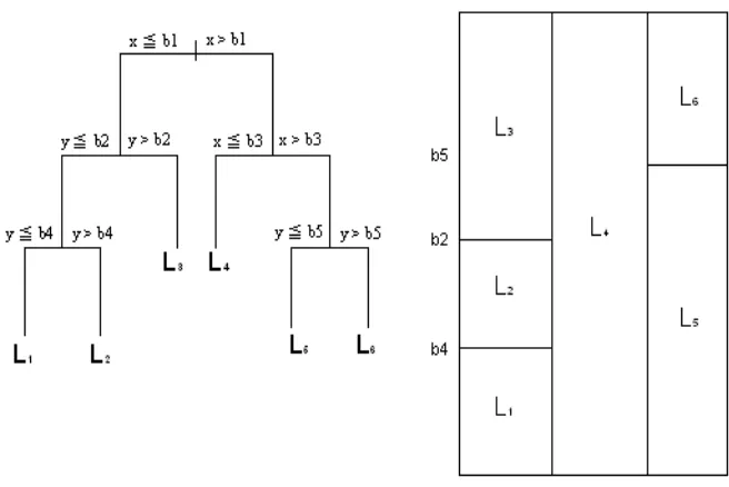
After growing a tree, we train an SVM on each of its leaves, using samples that flow to each leaf as training data (Figure 1). The values of the SVM parameters are also determined in a data-driven fashion. A tree and all SVMs associated with its leaves constitute a DTSVM classifier, as shown in Figure 1. In the training phase, all the SVMs in a DTSVM classifier are trained with the same parameter values. We explain how the optimal values are obtained in Section 2.2. In the validation/testing process, we first input a given validation/test object x to the tree. If x reaches a leaf that contains homogeneous samples, we classify x as the label of those samples; otherwise, we classify it with the SVM associated with that leaf.
2.2 The DTSVM Training Process
Given a training and validation component, we build a DTSVM classifier on the training component and determine its optimal parameter values with the help of the validation component. The param-eters associated with a DTSVM classifier are: (i)σ, the ceiling size of the decision tree; and (ii) the SVM parameters. Their optimal values are determined in the following manner.
We begin by training a binary tree with an initial ceiling size σ0, and then train SVMs on the
Figure 1: The architecture of a DTSVM classifier: a tree and all its leaves (L1 to L6) are produced and SVMs are trained on the leaves.
Next, we want to construct DTSVM classifiers with larger ceiling sizes, but we only train their associated SVMs with k top-rankedθ. To do this, we rankθin descending order of v(σ0,θ). LetΘk be the set that consists of k top-rankedθ.
More specifically, we implement the following sub-process, denoted as SubProcess(θ), for each
θ∈Θk.
1. Set t = 0 and get the binary tree with the ceiling sizeσ0.
2. Increase t by 1 and setσt=4×σt−1. Modify the tree with ceiling sizeσt−1to obtain a tree
with ceiling sizeσt. This is done by moving from the root towards the leaves and retaining each node whose parent’s size is greater thanσt. Then, train SVMs on the leaves with SVM-parametersθ. Let v(σt,θ)be the validation accuracy of the resultant DTSVM classifier.
3. If v(σt,θ)−v(σt−1,θ)≥0.5% andσt is less than the size of the training component, proceed to step 2.
4. Letσ(θ) =σt−1if v(σt,θ)−v(σt−1,θ)<0.5% orσ(θ) =σt ifσt is greater than or equal to the size of the training component.
When we have completed SubProcess(θ)for allθ∈Θk, we define
θopt=arg max
θ∈Θk
v(σ(θ),θ)andσopt=σ(θopt).
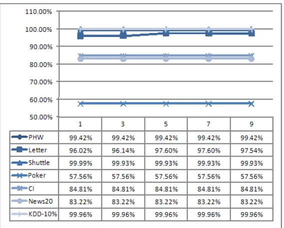
Figure 2: The test accuracy rates obtained by DTSVM on the seven data sets whenσ0= 1,500 and k = 1, 3, 5, 7 and 9.
Note that, in each SubProcess(θ), we setσt as quadruple the size (rather than double the size) ofσt−1 for two reasons. First, quadrupling the size produces more significant differences between v(σt,θ)and v(σt−1,θ), especially when t is small. This means that if a SubProcess terminates at a
small t, there is less risk of a low validation accuracy rate. Second, quadrupling the size enables the training process to progress at a faster pace. This means that if a SubProcess terminates at a large t, it moves more rapidly towards that end of the process.
The initial ceiling sizeσ0(=1,500) and the number k (=5) of the top-ranked parameters are set
heuristically. To observe how these settings impact the test accuracy, we first fix σ0 at 1,500 and
vary k from 1 to 9 at a step size of 2; we then plot the test accuracy rates obtained by DTSVM on the seven data sets whose details are shown in Table 1. Figure 2 shows that any value of k is good for all the data sets except “Letter”, while k = 5 or 7 is particularly good for “Letter”. Moreover, setting the right value of k improves the test accuracy of “Letter” significantly. Next, we fix k at 5 and varyσ0from 500 to 3,000 with a step size of 500. As shown in Figure 3, varying the value of σ0does not affect the test accuracy of any data set significantly.
3. Experimental Results
Figure 3: The test accuracy rates obtained by DTSVM on the seven data sets when k = 5, andσ0=
500, 1,000, 1,500, 2,000, 2,500 and 3,000.
3.1 The Data Sets
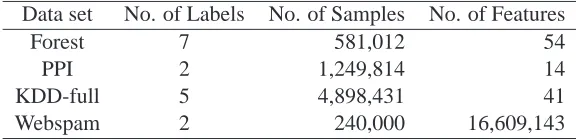
In the experiments, we divided the data sets into two groups. The first group was used to evaluate the efficiency of DTSVM and some alternative methods in terms of speeding up SVM training. The second group was used to verify that the DTSVM method could handle much larger data sets, for which most of the alternative methods required an excessive amount of time to complete the training process. The first group comprised seven medium-size data sets, ranging from 10K to 494K in size, as shown in Table 1. Most of the data sets have less than 50 features, but the “News20” has 62,060 features. The second group comprised four large-size data sets, ranging from 240K to 4,898K in size, as shown in the Table 2. The “Webspam” data set is not very large in terms of the number of samples (240K), but the number of features is more than 16M; thus, we consider it a large-size data set. All the data sets were obtained from UPI repository (Newman et al., 1998), with the following two exceptions: “PPI”, which was used in a protein-protein interaction study (Tseng et al., 2010), and “Webspam”, which was obtained from
http://www.cc.gatech.edu/projects/doi/WebbSpamCorpus.html
Note that the actual “Poker” data set in the repository contains 1 million samples; however, we only used its training component in our experiments.
Data set No. of Labels No. of Samples No. of Features
Pen Hand Written (PHW) 10 10,992 16
Letter 26 20,000 16
Shuttle 7 58,000 9
Poker 10 25,010 10
Census Income (CI) 2 45,222 14
News20 20 19,927 62,060
KDD CUP 10% (KDD-10%) 5 494,021 41
Table 1: The medium-size data sets used in our experiments.
Data set No. of Labels No. of Samples No. of Features
Forest 7 581,012 54
PPI 2 1,249,814 14
KDD-full 5 4,898,431 41
Webspam 2 240,000 16,609,143
Table 2: The large-size data sets used in our experiments.
http://ocrwks11.iis.sinica.edu.tw/dar/Download/DataSets/DTSVM/datasets.htm
In each data set, we normalized all the feature values to a real number between 0 and 1. We did this by transforming each value v of feature f into(v−fmin)/(fmax−fmin), where fmaxand fminare the maximum and minimum values of f respectively.
We only studied non-linear SVMs in our experiments. Moreover, we used the RBF kernel function to measure the similarity between vectors. As a result, we had two SVM parameters: the penalty factor C, whose values were taken fromΦ={10a: a=−1,0, . . . ,5}; and theγparameter in the RBF function, whose values were taken fromΨ={10b: b=−4,−3, . . . ,4}. Thus, the set of all SVM parameter values wasΘ=Φ×Ψ, which comprised 63 pairs of values for(C,γ).
SVM training is implemented under the 1A1 and 1AO approaches. When the 1A1 approach is used, there are n(n−1)/2 classifiers, where n is the number of labels. Each classifier assigns one of two possible labels to a given validation/test sample. We use all the classifiers to classify a given validation/test sample x, based on a majority vote. Note that a more efficient technique (Platt et al., 2000) that only requires n classifiers can be used in the validation/testing procedure. However, we adopt Knerr et al.’s (1990) technique, which requires n(n−1)/2 classifiers, because we are only interested in the relative, rather than the absolute, performance of the methods compared in our experiments. When the 1AO approach is used, there are n decision functions, each of which is associated with a label. We assign x the label associated with the decision function that yields the highest functional value.
3.2 Methods Compared
CART. CART (Breiman et al., 1984) is similar to the decomposition scheme used in DTSVM,
but it differs in terms of the stop and classification criteria. In the training phase, CART stops splitting a node when IR(f,v) =0 for all features f and their values v. In the testing phase, it classifies a test sample x by the label shared by the majority of samples residing at the leaf to which x flows. Although CART is not designed for speeding up SVMs, it serves here as a benchmark for DTSVM. If CART performs as well as DTSVM in every respect, then there is no need for DTSVM, since CART runs much faster than DTSVM in both the training and testing phases.
RDSVM. RDSVM (randomized SVM) is an alternative to DTSVM that differs from DTSVM in
the way it decomposes a data space. In the training phase, when a sizeσis given, DTSVM randomly assigns a training sample to one of d subsets, where d is the smallest integer that is greater than or equal to n/σand n is the number of training samples. RDSVM uses the same procedure as DTSVM to search for the optimal parameters. In the testing phase, RDSVM randomly assigns a test sample to a subset and classifies it according to the SVM associated with that subset.
Bagging. When implementing bagging (Breiman, 1996), we created a number of SVMs for
eachθ∈Θ. Each SVM was trained on 1,500 training samples chosen at random. For eachθ, the training was conducted sequentially. We stopped at the first m so that the validation accuracy rate of m SVMs did not exceed that of m−1 SVMs by more than 0.5%.
CBD. The training process of CBD (Panda et al., 2006) comprises two steps: finding a reduced
set, and training an SVM on that set for eachθ∈Θ. The first part involves finding the k-nearest neighbors of each training sample and deriving the reduced data set via a down-sampling technique. Following Panda et al. (2006), we set k at 100. When searching for the 100 nearest neighbors of each training sample x, we keep the current list of 100 nearest neighbors of x. For another training sample z, let d(x,z)be the distance between x and z. We need to compare this distance with d(x,w), where w is on the current list and has the largest distance with x. Since the squared distance is the sum of the squared feature differences, we can speed up the comparison by computing the partial sum of d2(x,z). When this partial sum exceeds d2(x,w), we stop the comparison and exclude z
from the current list of x.
LIBSVM. LIBSVM (Fan et al., 2005) is now the most widely used software for training and
testing SVMs. We take it as the baseline in our experiments; thus, the speedup factor is 1 by assumption. If a compared method is faster in training than LIBSVM, it has a speedup factor above 1.
LASVM. LASVM (Bordes et al., 2005) is a method that solves a dual optimization problem by
way of a stochastic gradient descent method that converges to an optimal solution in one examina-tion of the training samples.
LIBLINEAR. LIBLINEAR (Fan et al., 2008) is a fast version of training and testing linear
SVMs. Its training speed is comparable to, or even faster than, that of Pegasos (Shalev-Shwartz et al., 2007) and SVMperf (Joachims, 2006). Since LIBLINEAR is not a method for speeding up non-linear SVMs, we only include it in our experiments for large-size data sets, for which bagging, CBD, LIBSVM and LASVM take too long to complete the training process. When we train linear SVMs, the values of the penalty factor C are taken fromΦ={10a: a=−1,0, . . . ,5}, which com-prises 7 real numbers. Furthermore, we require the discriminant function of the classifier to include a bias term.
3.3 Results on Medium-Size Data Sets
The results of applying seven methods, CART, DTSVM, RDSVM, bagging, CBD, LIBSVM and LASVM, to the seven medium-size data sets are shown in Figures 4-8 for 1A1 training, and in Figures 9-13 for 1AO training. In all SVM training sessions, except for LASVM, we used the LIBSVM software (Fan et al., 2005). We adopted all default options of the software, except the parameter values, which we specified in Section 3.1.
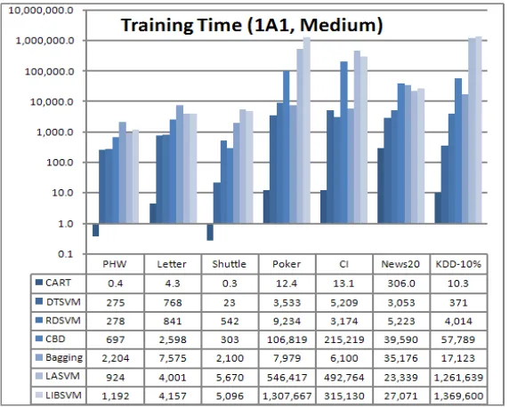
Figure 4 and Figure 9 show the training times of the seven methods. The training time of each method comprises the time required to obtain reduced data sets if it is a data reduction method, the time to train all SVMs and the time to search for optimal parameters; however, the time required to input or output data is not included. The computation for all the medium-size data sets was performed on an Intel Xeon CPU 3.2 GHz with a 2GB RAM, while that for all the large-size data sets was performed on a Quad-Core Intel Xeon X5365 3.0GHz CPU and 32GB RAM.
Figure 5 and Figure 10 show the speedup factors of all the methods except LIBSVM, where the speedup factor of a method
M
is computed as LIBSVM’s training time divided byM
’s training time.Figure 6 and Figure 11 show the test accuracy rates of the four compared methods. Note that the DTSVM test accuracy is that of the DTSVM classifier with the ceiling size σopt and SVM-parameters θopt. When classifying a test sample with SVMs, the most time-consuming part is computing a decision function, whose complexity can be measured in terms of how many SVs are encountered in the classification. Therefore, we use the “number of encountered support vectors” (NESV) as a measure of the time-complexity of the test process. NESV is defined as the number of SVs contained in the decision function used to classify a test sample. When a DTSVM or an RDSVM classifier is used, the NESV is associated with the leaf that the test sample flows to. Thus, in the two cases, NESV is the average number of SVs encountered by a test sample.
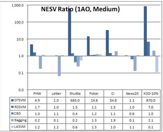
Figure 7 and Figure 12 list the NESVs of the four methods; while Figure 8 and Figure 13 show the NESV ratios of all the methods except LIBSVM and CART, where the NESV ratio of a method
M
is computed as LIBSVM’s NESV divided byM
’s NESV. We now summarize the results shown in Figures 4 to 13.1. There is no doubt that CART was extremely fast in training, but its test accuracy was poor, except on the “Shuttle” and “KDD-10%” data sets, where its accuracy matched the best of all the other methods.
2. In terms of training time, DTSVM outperformed all the other methods, except CART; and in terms of test accuracy and NESV, DSTVM outperformed or performed comparably to all the other methods. It also achieved very large speedup factors and NESV ratios on “Shuttle”, “Poker”, “CI” and “KDD-10%”.
3. RDSVM, being an alternative approach to DTSVM, achieved comparable test accuracy to DTSVM. However, it performed worse in terms of training time on “Shuttle”, “Poker” and “KDD-10%”. It also performed worse in terms of NESV on “Shuttle”, “Poker”, “CI” and “KDD-10%”.
Figure 4: Training times of the seven compared methods, expressed in seconds. Training type = 1A1. CART, DTSVM and RDSVM outperformed the other methods.
Figure 6: Test accuracy rates of all the methods. Training type = 1A1. CART performed poorly on several data sets; while CBD and Bagging lagged behind DTSVM on some data sets.
Figure 8: The NESV ratios of all the methods except CART and LISBSM. Training type = 1A1. DTSVM outperformed all the other methods.
Figure 10: Speedup factors of all the methods except LIBSVM. Training type = 1AO. CART, DTSVM and RDSVM outperformed the other methods.
Figure 12: The NESVs of all the methods except CART. Training type = 1AO. DTSVM outper-formed all the other methods.
PHW Letter Shuttle Poker CI News20 KDD-10%
1A1 DTSVM 7,694 183,450 181 88,935 8,975 207,290 1,638
LIBSVM 8,073 183,450 1,134 140,990 10,451 210,560 2,287
1AO DTSVM 1,775 16,200 195 42,775 8,975 39,122 1,580
LIBSVM 1,210 16,201 266 39,024 10,451 42,628 1,566
Table 3: The total number of SVs produced by DTSVM and LIBSVM on medium-size data sets. The two methods produced about the same numbers of SVs, even though DTSVM has much smaller NESVs than LIBSVM.
5. Bagging achieved speedup factors below 1 and NESV ratios below 1 on several data sets. It also lagged behind DTSVM in terms of test accuracy on “Letter” and “News20”.
6. LASVM, being an alternative numerical method to LIBSVM, achieved speedup factors slightly above 1 on most data sets, but its scores were much lower than those of DTSVM. LASVM also achieved NESV ratios above 1 on most data sets, although they were generally not as high as those of DTSVM. An unexpected result occurred in the 1AO training on “KDD-10%”, where LASVM obtained very high NESVs compared to LIBSVM, resulting in a low NESV ratio (0.1). We double checked the process to confirm that the above result was correct.
Finally, we provide some additional information about DTSVM. In Table 3, we show the total
number of support vectors (TNSV) produced by DTSVM and LIBSVM on all medium-size data
sets. TNSV expresses the space-complexity of a training process, whereas NESV expresses the time-complexity of a test process. For DTSVM, the NESV is smaller than the TNSV in most cases, because a test sample usually encounters only some, rather than all, SVs. For LIBSVM, NESV is always the same as TNSV. Note that DTSVM achieved much smaller NESVs on many data sets, but it produced about the same TNSV on all the data sets.
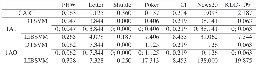
Table 4 shows the DTSVM testing times, as well as the LIBSVM and CART testing times for comparison. As expected from the NESV results, DTSVM’s testing time is shorter than that of LIBSVM on all the data sets. We further divide DTSVM’s testing time into the time spent on the decision-tree component (DTC) and that spent on local SVMs (lSVMs). In Table 4, the times are separated by a semi-colon. Clearly, the DTC testing time takes an extremely small proportion of DTSVM’s testing time. In fact, it is so small that it cannot be measured accurately by the timing mechanism. CART’s testing time, on the other hand, is higher than that of the DTC because CART-trees usually grow to deeper levels than DTC-CART-trees.
3.4 Results on Large-Size Data Sets
The results of applying four methods, CART, DTSVM, RDSVM and LIBLINEAR, to the four large-size data sets are shown in Figures 14-16 for 1A1 training, and in Figures 17-19 for 1AO training. Once again, we used the LIBSVM software for all SVM training sessions of DTSVM and RDSVM.
We summarize the results on large-size data sets as follows.
PHW Letter Shuttle Poker CI News20 KDD-10%
CART 0.063 0.125 0.360 0.157 0.204 0.093 2.187
DTSVM 0.047 3.844 0.000 0.406 0.219 38.141 0.063
1A1 0; 0.047 0; 3.844 0; 0.000 0; 0.406 0; 0.219 0; 38.141 0; 0.063
LIBSVM 0.265 4.078 0.187 7.406 8.453 39.062 7.344
DTSVM 0.062 7.344 0.000 1.125 0.219 126 0.063
1AO 0; 0.062 0; 7.344 0; 0.000 0; 1.125 0; 0.219 0; 126 0; 0.063
LIBSVM 0.328 7.328 0.250 17.313 8.453 138.000 19.875
Table 4: The testing time required by CART, DTSVM and LIBSVM on medium-size data sets. The time required by DTSVM is lower than that required by LIBSVM. The DTC testing time takes a very small proportion of DTSVM’s testing time. CART’s testing time is higher than that of DTC.
Figure 14: Training times of the four methods, expressed in seconds. Training type = 1A1. CART and LIBLINEAR outperformed the other methods.
and RDSVM on “Forest” and “PPI”, and surpassed CART on “PPI” by a significant margin. Moreover, DTSVM achieved much lower NESVs than RDSVM on all the data sets.
2. Recall that RDSVM achieved equally good test accuracy rates on all the medium-size data sets. However, on the large-size data sets, it achieved much lower accuracy rates on “Forest” and “PPI”, and it yielded much higher NESVs on all the data sets. The results show that RDSVM is not a good substitute for DTSVM in solving large-scale SVM problems.
3. The results also show that, despite their efficiency in training, CART and LIBLINEAR are
not good substitutes for DTSVM in solving large-scale problems. LIBLINEAR achieved the
Figure 15: Test Accuracy of the four methods. Training type = 1A1. DTSVM outperformed, or performed comparably to, the other methods. CART performed rather well compared to LIBLINEAR.
Figure 16: The NESVs of DTSVM and RDSVM. Training type = 1A1. DTSVM achieved much lower NESVs than RDSVM.
rather well. However, to verify this assumption, we need to compare the test accuracy rates of linear and non-linear models. DTSVM offers us an opportunity to make such a comparison.
Figure 17: Training times of the four methods, expressed in seconds. Training type = 1AO. CART and LIBLINEAR outperformed the other methods.
Figure 18: Test Accuracy of the four methods. Training type = 1AO. DTSVM outperformed, or performed as well as, the other methods.
3.5 Further Discussion
To gain insight into why DTSVM is so effective, we show in Table 7 theσopt derived by DTSVM on medium-size data sets, along with the proportion of training samples that flow to homogeneous leaves. Note that a single table suffices to show all the results because 1A1 training and 1AO training employ the same decision trees and DTSVM yields the sameσopt value for both approaches.
Figure 19: The NESVs of DTSVM and RDSVM. Training type = 1AO. DTSVM achieved much lower NESVs than RDSVM.
Forest PPI KDD-full Webspam
DTSVM 1A1 140,008 594,687 2,752 8,116
1AO 114,958 594,687 2,781 8,116
Table 5: The total number of SVs produced by DTSVM on large-size data sets.
Forest PPI KDD-full Webspam
CART 0.109 0.563 0.281 151.860
1A1 2.485 38.453 1.094 127.000
DTSVM 0.047; 2.438 0.235; 38.218 0.25; 0.844 75; 52.000
1AO 3.859 38.453 1.485 127.000
0.047; 3.812 0.235; 38.218 0.25; 1.235 75; 52.000
Table 6: The testing time required by CART and DTSVM on large-size data sets. DTC’s testing time only takes a very small proportion of DTSVM’s testing time. CART’s testing time is higher than that of DTC.
PHW Letter Shuttle Poker CI News20 KDD-10%
σopt 1,500 24,000 1,500 1,500 1,500 24,000 1,500
Proportion 0% 0% 98.42% 0% 15.76% 0% 97.35%
PHW Letter Shuttle Poker CI News20 KDD-10%
1A1 DTSVM 1,500 24,000 1,500 1,500 1,500 24,000 1,500
RDSVM 1,500 24,000 1,500 24,000 6,000 24,000 1,500
1AO DTSVM 1,500 24,000 1,500 1,500 1,500 24,000 1,500
RDSVM 1,500 24,000 1,500 24,000 24,000 24,000 1,500
Table 8: Theσopt values derived by DTSVM and RDSVM on the medium-size data sets.
Data Set Training Mode 1,500 6,000 24,000
Letter 1A1 633 45 90
1AO 2,730 178 373
News20 1A1 1,631 665 757
1AO 7,056 2,952 3,365
Table 9: The DTSVM training times required for different ceiling sizes.
Data Set Training Mode 1,500 6,000 24,000
Letter 1A1 95.35% 96.61% 97.60%
1AO 95.71% 96.91% 97.66%
News20 1A1 67.02% 76.92% 83.22%
1AO 70.82% 79.06% 84.34%
Table 10: The DTSVM test accuracy rates that correspond to different ceiling sizes.
in any homogeneous leaves, DTSVM achieved very high speedup factors and NESV ratios on these two data sets. The same fact also explains why DTSVM achieved such low NESVs, which even fell below 1 on “Shuttle”. Note that this phenomenon occurs because decision trees group neighboring samples into the same leaf. RDSVM, on the other hand, does not produce the same effect because the probability that all samples will carry the same label in the same randomly decomposed region is extremely small.
The lack of homogeneous leaves is not the only reason for RDSVM’s poor performance in training. Table 8 shows theσopt values derived by DTSVM and RDSVM. The results explain why RDSVM achieved much smaller speedup factors and NESV ratios on “CI” and “Poker”.
Forest PPI KDD-full Webspam
σopt 1,500 1,500 1,500 1,500
Proportion 5.55% 1.64% 42.05% 80.63%
Table 11: Theσopt values obtained by DTSVM on the large-size data sets and the proportion of training samples that flowed to homogeneous leaves.
Forest PPI KDD-full Webspam
1A1 DTSVM 1,500 1,500 1,500 1,500
RDSVM 96,000 1,500 1,500 96,000
1AO DTSVM 1,500 1,500 1,500 1,500
RDSVM 1,536,000 1,500 1,500 96,000
Table 12: Theσopt values obtained by DTSVM and RDSVM on the large-size data sets.
Table 9 shows the training times required for different ceiling sizes. We observe that DTSVM spent most of its time on the leaves with the lowest ceiling size. In addition, Table 10 shows the test accuracy rates corresponding to different ceiling sizes, assuming that the training was terminated at those sizes. The results demonstrate the benefit of searching for theσopt because, if we terminated the training at ceiling size 1,500 or 6,000, we would obtain significantly lower test accuracy rates.
Thus far, we have only discussed the DTSVM results for medium-size data sets. For complete-ness, Table 11 shows theσoptvalues obtained by DTSVM on the large-size data sets, along with the proportion of training samples that flowed to homogeneous leaves. In Table 12, we show theσopt values obtained by DTSVM and RDSVM. The results explain why RDSVM required much longer training times and more NESVs for “Forest”, “PPI” and “Webspam”.
Since DTSVM’sσopt=1,500 for all four data sets, we do not have any tables for the large-size data sets correspond to Tables 9 and 10 for the medium-size data sets.
4. Generalization Error Bounds for the DTSVM Classifier
To provide a generalization error bound of DTSVM, we start with the following framework. Let Rd be the d-dimensional Euclidean space. We assume that a set of training examples Xn =
{(x1,y1), . . . ,(xn,yn)}is given, where(xk,yk)∈Rd×{−1,1}for k=1, . . . ,n. The DTSVM method produces a classifier h(x,π,f), in which πis a binary tree comprised of L leaves, f= (f1, . . . ,fL), and fi is related to the lSVM trained on leaf i of πfor i=1, . . . ,L. The binary treeπ produces a partition function that maps an input in Rd to{1, . . . , L}, and let π(x) be the leaf that x flows to. On the other hand, the lSVM trained on leave i, i=1, . . . ,L is expressed as fi◦Φ, whereΦmaps an input in Rd to a Hilbert space H, and fi is a linear function from H to R. Note that for a linear function g : H→R, there exists some w∈H such that
g(z) =hw,zi
Note that if π(x) =i, then h(x,π,f) =sign(fi(Φ(x)). Let us define the function fπ: Rd →
{−1,1}by
fπ(x) = fπ(x)(Φ(x)).
It follows that h(x,π,f) =sign(fπ(x)).
Sometimes,Φ is only defined implicitly. That is, instead of specifying the functional form of
Φ, only the inner product ofΦ(u)andΦ(v)is specified as
hΦ(u),Φ(v)i=k(u,v),
where u,v∈Rd , and k(·,·)is a kernel function. In the remainder of this section, we assume that the functionΦis given and fixed.
Next, we define several notations used in this section. N is the set of natural numbers; R+ is the set of positive real numbers;
P
L(Rd)is the class of all functions from Rd to{1, . . . ,L};R
(H) is the class of all functions from H to R; andL
(H)is the class of all linear functions from H to R. Moreover, if T is a set, we define TL={(t1, . . . ,tL): ti∈T for i=1, . . . ,L}; that is, TLcomprises all the L-tuples of T ’s elements.To provide a bound for the generalization error of h(x,π,f), we need the standard notions of shatter coefficients, margins and covering numbers, which are defined below. Further details can be found in Vapnik (1995) and Cristianini and Shawe-Taylor (2000). First, we define the notion of the shatter coefficient, which we use to measure the complexity of the partition functions corresponding to binary decision trees. Informally, the nthshatter coefficient of a class
G
⊆P
L(Rd)is the maximum number of ways in which n points can be partitioned into L parts by functions inG
. Formally, we have the following definition.Definition 1 Let
G
⊆P
L(Rd). For any n∈N, the nthshatter coefficient ofG
isV(
G
,n) = maxS⊆Rd,|S|=n|{πS:π∈
G
}|,whereπSis the function obtained by restrictingπto the domain S.
Next, we extend the standard notion of the margin to a collection of margins, one for each part of a partition, in the following way.
Definition 2 Let f= (f1, . . . ,fL)∈(
R
(H))L,π∈P
L(Rd), Xn⊆Rd×{−1,1}, andγ= (γ1, . . . ,γL)∈(R+)L. We say that fπhas marginγon X
n, or mg(fπ,Xn)≥γ, if
y·fπ(x)≡y·fi(Φ(x))≥γi
for any i∈ {1, . . . ,L}and any(x,y)∈Xnwithπ(x) =i.
Definition 3 Let η∈R+ and
F
⊆R
(H). For a subset D⊆H, letC
(F
,D,η) be the smallest collection of functions from D to R such that, for each f ∈F
, we have g∈C
(F
,D,η)with|f(z)− g(z)| ≤ηfor each z∈D. For E⊆H and n∈N, we define the covering number ofF
with respect to E, n andηasN(
F
,E,n,η) = maxD⊆E,|D|=n|
C
(F
,D,η)|.4.1 Hard Margin Bounds
We have a set Xn of n training examples drawn independently and at random according to the distribution
D
. Moreover, we have a learned classifier sign(fπ), withπ∈P
L(Rd)and f ∈(R
(H))L, which classifies all the training examples correctly with a large margin. Our objective is to bound thegeneralization error of the classifier sign(fπ), which is defined as the probability that sign(fπ(x))6= y, with(x,y)sampled according to
D
. The following lemma gives such a bound, which generalizes a known result for SVMs (cf. Cristianini and Shawe-Taylor, 2000).Lemma 4 Let
G
⊆P
L(Rd),γ= (γ1, . . . ,γL)∈(R+)L, andF
=F
1× ··· ×F
L, whereF
i⊆R
(H)for 1≤i≤L. In addition, let
D
be a probability distribution on Rd× {−1,1}, and let n be a large enough integer. Suppose a set of n samples Xnare drawn independently and at random accordingto
D
, and consider any classifier sign(fπ), withπ∈G
and f∈F
, such that mg(fπ,Xn)≥γ. Then,with probability 1−δ, the generalization error of mg(fπ)will be at most
2
n "
L
∑
i=1log N(
F
i,E,2n,γi/2) +logV(G
,2n) +log(2/δ)#
,
where E={Φ(x):(x,y)∈supp(
D
)}and supp(D
)is the support ofD
.We provide the proof in Appendix A, as it is rather lengthy and closely follows the standard approach and that of Cristianini and Shawe-Taylor (2000). The idea is to show that the functions fπ, withπ∈
G
and f∈F
, can be “well covered” by a small number of functions, so that a union bound can be applied to provide an upper bound on the probability that our classifier has a large generalization error.Before proceeding further, we explain the meaning of Lemma 4. Suppose for some
G
andF
=F
1× ··· ×F
L, we can build a classifier sign(fπ)withπ∈G
and f∈F
that has a large marginand zero training error. Then, Lemma 4 gives us an upper bound on the generalization error of
sign(fπ) in terms of the complexity of
G
andF
i, where we measure the complexity ofG
by its shatter coefficient V(G
,2n)and the complexity of eachF
iby its covering number N(F
i,E,2n,γi/2). To obtain a small generalization error, we need to have aG
with a small V(G
,2n)and anF
i with a small N(F
i,E,2n,γi/2). However, this does not suggest that we can simply choose anyG
andF
i with small V(G
,2n)and N(F
i,E,2n,γi/2)for any classification task. This is because we may not be able to build a classifier fromG
andF
ito classify every training example correctly with a large margin. For example, if we do not chooseG
properly (say, by using a random partition), the training examples in some parts of the partition may not be separated by SVMs with a large margin. Our main contribution is the discovery that decision trees are good partition functions when combined with SVMs, since they allow a large margin and only require a short training time for lSVMs.L
(H,β)as the class of all linear functions f ∈L
(H)withkfk ≤β. A bound can be obtained for the covering number ofL
(H,β)with respect to E, n andη, provided that E is a bounded subset of H (see, for example, Bartlett and Shawe-Taylor, 1998). This shows that, although there is an infinite number of functions inL
(H,β), they can be covered by a small number of functions inR
(H)with respect to any set of n points in E. As a result, the complexity of the classL
(H,β) is low when measured by its covering number.Lemma 5 Letα,β,η∈R+and let n∈N. Consider any E⊆H withkzk ≤ρfor every z∈E. Then, there is a constant c such that
log N(
L
(H,β),E,n,η)≤cρ 2β2 η2 log2n.
We also define
B
L(Rd)as the class of partition functions associated with binary trees containingL leaves that partition the space Rd into L axis-aligned parts, as described in Section 2. Clearly,
B
L(Rd)⊆P
L(Rd). The following lemma provides a bound on the nthshatter coefficient ofB
L(Rd). Lemma 6 Let d,n,L∈N. ThenV(
B
L(Rd),n)≤L log(dnL2).Proof Consider any n-element subset S⊆Rd. We need to cut S into L parts. Initially, there is only one part in S. We perform the cut operation iteratively in the following way. Each time, we choose one part from at most L−1 existing parts of S and cut it into two parts. To do this, we pick one of the d dimensions and at most one of the n−1 cutting hyperplanes on that dimension. Thus, there are at most(L−1)d(n−1)≤dnL ways to perform one cut operation. To obtain L parts, we repeat
the cut operation L-1 times; hence, the number of possible partitions is at most(dnL)L−1≤(dnL)L. Finally, there are L! ways to order the L parts of each partition, yielding the following result:
V(
B
L(Rd),n)≤(dnL)L·(L!)≤(dnL2)L.From the above three lemmas, we immediately derive the following theorem.
Theorem 7 Letρ∈R+,βi∈R+for 1≤i≤L,γ= (γ1, . . . ,γL)∈(R+)L, and
F
=L
(H,β1)× ···×L
(H,βL). In addition, letD
be a probability distribution on Rd× {−1,1}such thatkΦ(x)k ≤ρfor every (x,y)∈supp(
D
), and let n be a large enough integer. Suppose a set Xn of n samplesare drawn independently and at random according to
D
, and consider any classifier sign(fπ), with π∈B
L(Rd)and f∈F
, such that mg(fπ,Xn)≥γ. Then, with probability 1−δ, the generalizationerror of sign(fπ)will be at most
c n
L
∑
i=1ρ2β2
i
γ2
i
log2n+L log(dnL2) +log(1/δ) !
,
From Theorem 7, we conclude that if a classifier partitions the training data set into a small number of parts (i.e., L is sufficiently small), and it classifies each training sample with a large margin (i.e.,γi is large for each i), then the classifier is likely to have a small generalization error. However, this theorem does not indicate how to find a good value for L because, in general, it is hard to know how L affects the margins and the generalization error bound. Instead of being led by any analytical result, the DTSVM learning algorithm takes a data driven approach to find a good L. Note that the bound in Theorem 7 has a similar form to the generalization error bound of the perceptron decision trees proposed by Bennett et al. (2000). The main difference is that in their bound,γiis the margin at the ithinternal node and the sum is over all the internal nodes. We remark that it is hard to tell which one of these two bounds is better because, in general, we do not know their actual values for different learning tasks.
4.2 Soft Margin Bounds
Note that Theorem 7 works in the case where the training data Xn can be separated with a mar-gin vector γ. If the data is non-separable or noisy, we need to consider the notion of a soft margin (Cristianini and Shawe-Taylor, 2000). Suppose we have π∈
P
L(Rd), which partitionsXn into L parts: Xn1, . . . ,X
(L)
n , where Xn(i) ≡ {(x,y) ∈Xn :π(x) = i}, and let us denote Xn(i)=
{(xi,1,yi,1), . . . ,(xi,ni,yi,ni)} for some ni ∈N, for 1≤i≤L. In addition, suppose we have f=
(f1, . . . ,fL)∈
L
(H,β1)× ··· ×L
(H,βL), whereβi ∈R+ for 1≤i≤L. Then, we can define the margin slack vector of fias follows.Definition 8 Letγ= (γ1, . . . ,γL)∈(R+)L. For 1≤i≤L and 1≤ j≤ni, let
ξi,j=max(0,γi−yi,j·fi(Φ(xi,j))).
The definition reflects how far the elements of Xn(i)are from having a marginγi. Therefore, for 1≤i≤L, we call the vectorξi= (ξi,1, . . . ,ξi,ni)the margin slack vector of fiwith respect toπand
γiover Xn.
To find a bound for the generalization error of sign(fπ)in the case of such a soft margin, we follow the approach of Shawe-Taylor and Cristianini (1999, 2002), which works for the case of
L=1. The idea is to map points of H to a higher dimensional space ˆH so that, for each i, the image of Xn(i)can be separated by some function ˆfiwith the desired margin. Theorem 7 can then be applied. To find each ˆfi, we present the following lemma, which is a simple extension of Shawe-Taylor & Cristianini’s approach. For completeness, we provide the proof in Appendix B.
Lemma 9 Suppose that kΦ(x)k ≤ρ for any (x,y)∈supp(
D
). Then, there exists a space ˆH, amapping τρ: H→H, and a sequence ˆfˆ = (f1ˆ, . . . ,fˆL) of L functions such that the following four
facts hold.
1. For any(x,y)∈supp(
D
),kτρ(Φ(x))k ≤√2ρ.2. For 1≤i≤L, ˆfi∈
L
(Hˆ,βˆi)with ˆβi≤q
β2
i +kξik2/ρ2.
3. For 1≤i≤L, any(xi,j,yi,j)∈Xn(i)will be classified correctly with a margin
4. For 1≤i≤L and for any(x,y)∈/Xn, ˆfi(τρ(Φ(x))) = fi(Φ(x)).
According to this lemma, we define
Ψ=τρ◦Φ, and
ˆfπ(x) = fˆπ(x)(Ψ(x)).
Then, we know that ˆfπhas a margin(γ1, . . . ,γL)on Xn. Moreover, for(x,y)∈supp(
D
), we havekΨ(x)k ≤ kτρ(Φ(x))k ≤√2ρ.
Now we can apply Theorem 7, with the space H replaced by ˆH and the mappingΦreplaced byΨ, to obtain a bound on the generalization error of sign(ˆfπ), but with the quantityρ2β2/γ2replaced by
2ρ2(β2
i +kξik2/ρ2)
γ2
i
=2(ρ 2β2
i +kξik2)
γ2
i
.
Finally, to bound the generalization error of sign(fπ), by Lemma 9, we know that for any(x,y)∈/ Xn, sign(fπ(x)) =sign(ˆfπ(x)); therefore, sign(fπ) and sign(ˆfπ)have the same generalization error for inputs that do not fall within Xn. However, it is possible that the elements of Xnmisclassified by
sign(fπ)take a nontrivial measure in D, which results in sign(fπ)having a larger generalization error over
D
than sign(ˆfπ). As suggested by Shawe-Taylor and Cristianini (2002), this can be handled by modifying sign(fπ)on the misclassified elements in Xn. We call this new function the Xn-filtered version of sign(fπ). Then, we have the following theorem.Theorem 10 Letρ∈R+,βi∈R+for 1≤i≤L,γ= (γ1, . . . ,γL)∈(R+)L, and
F
=L
(H,β1)×···×L
(H,βL). In addition, letD
be a probability distribution on Rd× {−1,1}such thatkΦ(x)k ≤ρfor every(x,y)∈supp(
D
), and let n be a large enough integer. Suppose a set of n samples, Xn,are drawn independently and at random according to
D
; and consider any π∈B
(Rd) and f= (f1, . . . ,fL)∈F
, such that for i≤i≤L, fihas a margin slack vectorξiwith respect toπandγioverXn. Then, with probability 1−δ, the generalization error of the Xn-filtered version of sign(fπ)will
be at most
c n
L
∑
i=1ρ2β2
i +kξik2
γ2
i
log2n+L log(dnL2) +log(1/δ) !
,
for some constant c.
Theorem 10 shows that if we can build a classifier with a small L and a small kξik for every
i, then the first two terms inside the parentheses of the bound will be small, and the classifier is
Data Set 1A1 1AO
T1 T2 T1 T2
PHW 1,699 55 5,769 55
Shuttle 1,152,495 110 2,756,183 110
CI 202,354 481 202,354 481
Poker 12,253 139 48,893 139
KDD-10% 1,297,678 287 64,238 287
Table 13: The values of two leading terms T1and T2 that appear in the generalization error bound
for DTSVM classifiers. Training types = 1A1 and 1AO.
4.3 A Numerical Investigation
Note that in Theorem 10,βi andγi are interdependent quantities for 1≤i≤L, so we can fix one of them and try to optimize the other. In the formulation of the SVM optimization problem, the objective is to minimizeβiunder the constraint thatγi=1 for 1≤i≤L. Under this convention, the bound in Theorem 10 becomes
c n
L
∑
i=1ρ2β2
i +kξik2
log2n+L log(dnL2) +log(1/δ) !
. (1)
Recall that a DTSVM classifier is associated with a tree with L leaves and each leaf is associated with an lSVM. If the tree has only one leaf (i.e., L=1), then the DTSVM classifier will be reduced to a gSVM classifier, which has the following generalization error bound
c n ρ
2β2+ kξk2
log2n+log(1/δ)
(2)
(cf. Cristianini and Shawe-Taylor, 2000).
Let us compare the terms that appear in parentheses in (1) and (2). The second term L log(dnL2)
in (1) is the shatter coefficient of the partition functionπassociated with a binary tree. We claim that the value of (1) achieved by DTSVM is dominated by the first term, which is the sum of L quantities associated with L leaves of a binary tree, as opposed to the single quantity in (2). Moreover, the first term in (1) achieved by DTSVM is comparable to the corresponding quantity in (2) achieved by gSVM. The following results confirm the above two claims.
To validate the first claim, we compare the two leading terms in parentheses in (1). The first term is T1=∑Li=1(ρ2β2i +kξik2)log2n and the second term is T2=L log(dnL2). The results, shown
in Table 13, confirm the claim that T1 far exceeds T2 and (1) is dominated by T1. Note that we
compute T1under the following assumptions. (i) When the data set contains more than two labels, T1is taken as the average of the quantities over all classifiers. (ii) The value ofρis always 1 when
RBF kernels are involved. (iii) The value of kξik2 is obtained from the solution to the quadratic programming optimization problem. Further details can be found in Cristianini and Shawe-Taylor (2000), Section 6.1.2.
To validate the second claim, we compare R=∑Li=1(ρ2β2
Data Set 1A1 1AO
S R R/L S R R/L
PHW 74 133 17 326 450 56
Shuttle 114,786 75,630 5,402 593,967 180,990 12,928
CI 16,422 13,599 257 16,422 13,599 257
Poker 370 874 49 2,328 3,486 194
KDD-10% 100,227 70,796 2,212 5,089 3,505 110
Table 14: The values of S and R, which appear in the generalization error bound for gSVM and DTSVM classifiers respectively, and the values of R/L. Training types = 1A1 and 1AO.
gSVM classifiers (i.e., in (1) and (2)) with the common factor log2n removed from them. To ensure
a meaningful comparison between R and S, both classifiers have to take the same(C,γ)values, which we specify as the optimal values for gSVM. As a result, we had to train new DTSVM classifiers for some data sets, using the same decomposition schemes (i.e., the same binary trees and same ceiling sizes) as the old classifiers, but different(C,γ)values.
Table 14 shows the values of S, R and R/L, derived from five data sets. The “Letter” and
“News20” data sets are not included in the table because the DTSVM classifier using the designated values of(C,γ)would be the same as the gSVM on those data sets. It is clear that the values of R are as small as (less than 150), or of the same order of magnitude as, those of the corresponding S. In fact, S can be viewed as the slack-to-margin ratio and R as the sum of such ratios. The results show that each lSVM generates smaller slack-to-margin ratios than the corresponding gSVM, while the sum of lSVM ratios is comparable to the corresponding gSVM ratio. This explains why the test accuracy rates of DTSVM classifiers are comparable to those of gSVM classifiers.
5. Conclusion
We have proposed a method that uses a binary tree to decompose a given data space and trains an lSVM on each of the decomposed regions. The resultant DTSVM classifier can be constructed in a much shorter time than the gSVM classifier, and still achieve comparable accuracy rates to the latter. We also provide a generalization error bound for the DTSVM classifier. Using some data sets to compute the theoretical bounds for gSVM and DTSVM classifiers, we find that DTSVM classifiers generate comparable error bounds to those generated by gSVM classifiers. This finding explains why DTSVM classifiers can achieve more or less the same accuracy rates as gSVM classifiers.
Appendix A. Proof of Lemma 4
Let