http://www.sciencepublishinggroup.com/j/ajtas doi: 10.11648/j.ajtas.20180706.14
ISSN: 2326-8999 (Print); ISSN: 2326-9006 (Online)
The Performance of Model Fit Indices for Class
Enumeration in Multilevel Factor Mixture Models
Miao Gao
1, Walter Leite
2, Jinxiang Hu
31
College of Education, Nanjing Normal University, Nanjing, China
2College of Education, University of Florida, Gainesville, USA 3
School of Medicine, University of Kansas Medical Center, Kansas City, USA
Email address:
To cite this article:
Miao Gao, Walter Leite, Jinxiang Hu. The Performance of Model Fit Indices for Class Enumeration in Multilevel Factor Mixture Models.
American Journal of Theoretical and Applied Statistics. Vol. 7, No. 6, 2018, pp. 222-228. doi: 10.11648/j.ajtas.20180706.14 Received: October 2, 2018; Accepted: October 16, 2018; Published: November 1, 2018
Abstract:
Factor mixture models combine the common factor model and latent class analysis. Given that multilevel data structures are very common in educational and social research, the multilevel factor mixture model (ML FMM) is appropriate for analyzing nested measurement data when population heterogeneity is unobserved. This simulation study aims to investigate the performance of model fit indices with multilevel factor mixture models under various conditions. In data simulation, the five-items and one-factor model with between- and within-cluster was chosen. Two subgroups with the factor mean difference were simulated so two-class was the correct number of classes. To investigate the performance of information criterions, the following conditions were manipulated in this study: class separation, the intraclass correlation (ICC), sample size. For each of the generated dataset, one correct model and three mis-specified models were analyzed to fit the data. The results showed that class separation was an important factor on detecting the correct number of classes in multilevel factor mixture models. The proportion correct increases as the class separation gets larger. Although no single criterion is always best, AIC yield a more accurate model selection than aBIC and BIC overall. Only when class separation is large, aBIC is more trustworthy for model selection. The results of this study can provide the information for educational researchers interested in analyzing multilevel data when the heterogeneity of the population is unknown.Keywords:
Class Enumeration, Multilevel Factor Mixture Models, Information Indices, Likelihood Ratio Tests1. Introduction
Social science and educational research are often interested in the latent constructs and group comparisons. Recently, interest has extended beyond differences in known groups leading to exploration of classes of individuals that are unknown, so called latent classes. Factor mixture modeling (FMM) [1] is a widely accepted data analysis method when the population heterogeneity is not observed. It is a combination of the common factor model and latent class analysis. When modeling FMM, researchers need to specify a hypothesized number of classes that might be present in the data. The true number of classes, however, is unknown. Therefore, researchers must rely on fit indices and various performance indicators to identify the best fitting model among plausible alternative models.
The multilevel factor mixture model (ML FMM) is a statistical model that explores unobserved population heterogeneity with respect to latent variables when data are nested. It is based on the assumption that higher-level units belong to latent classes that differ in term of the parameters of the factor model specified for the lower-level units [2]. Thus the basic idea of ML FMM is that some of the model parameters are allowed to randomly vary across clusters.
1.1. Factor Mixture Models
model shown in Equations 1 and 2 also includes a covariate
i
x , which can be related to yi both directly and through the
mediation of
η
i.i y i y i i
y = + Λν η + Γ x +ε (1)
i ηxi i
η
= Γ +ς
(2)One application of the model above is as a multiple indicator multiple causes (MIMIC) model to detect differential item functioning (DIF). The CFA model is extended with a categorical latent class variable (C) to model unobserved population heterogeneity. cik equals to 1 if
participant i belongs to class k; otherwise, cik equals to 0.
ik k yk ik yk i ik
y =ν + Λ η + Γ x +ε (3)
ik ci ηk ix ik
η
= Α + Γ +ς
(4)The probability of belonging to each of the classes is predicted for each participant during the model estimation. This is expressed by using multinomial logistic regression.
1
( )
k k i
k k i
X
i i K
X
k e P C k x
e α γ α γ + + = = =
∑
(5)where
α
K =0 andγ
K =0 so that eα γk+ kXi =1. Particularly,covariate X predicts the log odds of the probability of belonging to a specific class k versus the probability of being the last or a reference class (the arbitrarily chosen Kth class).
( 1| ) ln
( 1| ) k k
ik i
c c i iK i
P c x
x
P c x
λ
=
= + Γ
=
(6)
The last part of the model incorporates observed categorical outcome variables (U) that are predicted by class membership. The regression on class membership is a logistic regression.
( 1 | ) ln
1 ( 1| ) j
ij i
u i ij i
P u c
c
P u c
=
= Λ
− =
(7)
where we have j=1, … , J binary outcomes U.
1.2. Multilevel Factor Mixture Model
The multilevel factor mixture model (ML FMM) can be extended from the single level FMM to model the nested data structure. Considering yij as a vector of all observed
dependent variable for person i in group j, the ML FMM, assuming one factor at within-level, is defined as follows [4]:
ij ij kj kj ij ij
y C k υ η ε
= = + Λ +
(8)
ij Cij k kj Bkj ij kjXij ij
η µ η ξ
= = + + Γ +
(9)
exp( )
( )
exp( )
kj kj ij ij
kj kj ij k
X
P C k
X α β α β + = = +
∑
(10)where ηij are normally distributed latent variables, εijand
ij
ξ are zero mean normally distributed residuals. By allowing parameters in within-level equations to be random, we can build the cluster-level model to get the multilevel part [4]:
j B j xj j
η = +µ η + Γ +ζ . (11)
1.3. Class Enumeration
A variety of studies investigated the issue of deciding on the number of classes in mixture modelling. The most commonly used information criterion is Akaike Information Criteria (AIC) [5, 6]. The usual form of AIC is
2 log 2 ,
AIC= − L+ p (12)
where log L is the value of the maximized likelihood and p is the number of parameters to be estimated.
Another commonly used criterion Bayesian Information Criteria (BIC) was proposed by Schwarz [7]
2 log log ,
BIC= − L+p n (13)
where n is the sample size. BIC has a consistent property that can lead to a correct choice of model as n get infinite large [8]. With this feature, Sclove [9] defined the adjusted BIC (aBIC) by replacing the sample size n in the original equation with the adjusted sample size n*, n* = (n+2)/24. Therefore, penalties in original information criterion are reduced in aBIC.
To date, there is no common acceptance of the information indices for determining the number of classes. For categorical LCA models, AIC is found to be not a good indicator and the aBIC perform better than BIC; for continuous LCA, the superiority of the BIC is more evident [10, 11]. Yang [8] also examined the performance of information indices showing that aBIC had notable success in selecting LCA models. The BIC performs well in multilevel CFA especially for continuous variables [12]. Nylund, et al. [13] also found that the BIC performed well for FMM and the aBIC was even better. A few researches indicate that the performance of information criteria heavily depends on the simulation factors [14].
ignored, but not included the multilevel mixture model. Therefore, the objective of this study is to investigate the performance of model fit indices in ML FMM under various conditions.
2. Methods
2.1. Data Generation
The five-items and one-factor model with between- and within-cluster was chosen for data simulation. Only outcome variable was simulated and investigated in this study. No covariate was included in either within-cluster level or between-cluster level. The within-level models are
ij ij kj kj ij ij
y C k υ η ε
= = + Λ +
(14)
ij Cij k kj ij
η µ ξ
= = +
(15)
exp( )
( )
exp( )
kj ij
kj k
P C k α
α
= =
∑
(16)where αkj is the expected odds of falling into a given
category versus the reference category. For the identification purpose, for a reference class K, the coefficient αkjwas set to
0 so exp(αkj) was 1. The between-level equation without
covariate is
j j
η = +µ ζ (17)
Two subgroups with the factor mean difference were simulated so two-class was the correct number of classes. The population parameters (Mahalanobis distance, MD and intraclass correlation, ICC) were set according to the conditions stated below. The standardized loading values at the between-level and within-level were all set to 0.8 since 0.8 was an acceptable reliable measure in practical research.
For item variance, the within-cluster variance and between-cluster item variance was dependent on the item ICC. The sum of within-cluster item variance and between-cluster item variance was set to 1. According to the following equation, the between-cluster item variance equals to ICC, the within-cluster item variance equals to 1 - ICC.
2
2 2
B
B W
ICC
σ
σ
σ
=
+ (18)
For factor variance, we set the within-level factor variance to 1, the within-level residual variance to 0.5 and between-level residual variances to 0. The between-between-level factor variance was calculated based on the following equation corresponding to each item ICC level.
2 2 2
2 2 2 2 2 2
*
( * ) ( * )
B B B
B B B W W W
ItemICC
λ
λ
λ
Φ + Ψ =
Φ + Ψ + Φ + Ψ (19)
where λ is the loading, Φ is the factor variance, and Ψ is the item residual variance.
By assuming normal distribution, data were generated in R
which was also used to call Mplus 7 to estimate the multilevel factor mixture models.
2.2. Conditions
To investigate the performance of information criterions, the following conditions were manipulated in this study: class separation, the intraclass correlation (ICC), sample size. The levels of conditions were selected based on previous research and reflect the applied situation.
2.2.1. Class Separation
Discrepancy among classes is represented by the multivariate Mahalanobis distance (MD). The MD is primarily a function of the between class standardized factor mean differences [11] and therefore, class separation was based solely on standardized factor mean differences as opposed to the MD. Lubke and Muthén found that greater discrepancy among classes as defined by MD leads to increased precision in class assignment in FMM [11]. However, little is known about the optimal degree of discrepancy in ML FMM. Standardized factor mean differences were manipulated to assess the impact of increasing class separation on the performance of the fit indices in ML FMM. The MD values chosen in this study were 0.5, 1.0, 1.5, 2.0 and 2.5.
2.2.2. ICC
In multilevel modeling, the ICC has been shown to play an important role in the relative bias of standard error and factor loading estimates. According to Preacher, Zyphur & Zhang [17] and Hox & Maas [18], the ICC values used to generate data were selected to be 0.1, 0.2 and 0.3. The corresponding between-level factor variances were 0.198, 0.445 and 0.763. The ICC values at 0.1, .02 and 0.3 are common to see in multilevel simulation studies as well as the practical educational researches.
2.2.3. Sample Size
The within-cluster sample size (n) was set to be 10 and 30; the number of clusters (K) was to be 30, 50 and 100. Previous research has recommended the within-cluster sample size to be at least 10 and between-cluster sample size to be at least 100 [19]. The large sample size is not always feasible in practical research, so the sample size chosen in this study is relatively small.
With fully crossed design, there are 5 3 2 3× × × =90 conditions. Each condition was replicated 100 times, thus there were 90 100× =9000 datasets.
2.3. Data Analysis
three mis-specified models, a total of four models, were analyzed to fit the data. The four models are as follows: Model 1 one-class ML FMM; Model 2 two-class ML FMM (correct number of classes); Model 3 three-class ML FMM; Model 4 four-class ML FMM. Mplus 7 was used to run data analysis.
The fit indices AIC, BIC and aBIC provided in Mplus were assessed in four models for each of the 9000 datasets. The advantage of Monte Carlo simulation studies is that the correct model is known and therefore, the performance of fit indices can be assessed. For AIC, BIC and aBIC indices, the lower the value is the better fit the model is. Take AIC for example, if the AIC is lowest in class=2 compared with class=1, class=3 and class=4, we say AIC indicates the best fit model of class=2 and lead to the correct model selection. The proportion of times that each fit index lead to the selection of correct model was calculated to represent the accuracy of fit indices.
3. Results
The likelihood-based fit indices for comparison among the specified models include AIC, BIC and aBIC. The fit indices were compared under various conditions that are latent mean differences, item ICC, the number of clusters and the within-cluster sample size. In this section, model convergence rates are reported first, followed by the performance of the fit indices.
Although 100 replications were attempted for each condition, the percentage of converged solutions varied across the conditions and models. Especially, a high percentage of non-convergence occurred more frequently in conditions with smaller latent mean difference and smaller sample. Model with more classes also attempted to have lower convergence rates. The overall convergence rate for each condition in four models was approximately 96%. For further data analysis, if any solution for any number of classes did not converge in each condition, we exclude the case for data analysis. Thus, 7763 out of 9000 cases were assessed for the performance of fit indices.
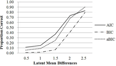
The proportion of times each of the AIC, BIC, aBIC led to selection of the correctly specified model among the
converged solutions was calculated for various condition. Figure 1 shows the proportion of correct identification of the two-class model for class separation at the level of 0.5, 1.0, 1.5, 2.0 and 2.5. Results showed that class separation was an important factor on detecting the correct number of classes in ML FMMs. The correct detection yield by AIC, BIC and aBIC ranged from approximately 10% to 90% as class separation increased. When class separation was 2 standard deviations, the proportion correct increased dramatically to 0.733, 0.417 and 0.681 for AIC, BIC and aBIC, respectively. When the class separation was 2.5 standard deviations, the proportion correct were 0.830, 0.794 and 0.903 for AIC, BIC and aBIC, respectively. As shown in Figure 1, when latent mean difference is smaller than 2, AIC performed better over BIC and aBIC; however, when latent mean difference is 2.5, aBIC had the best correct model detection.
Figure 1. Proportion correct by latent mean differences (D).
The impact of sample size varied slightly across the levels we studied. Figure 2 presented the proportion correct to detect the two-class models by the number of clusters and within-cluster sample size. Not surprisingly, when number of clusters (K) within-cluster sample size (n) increased, the proportion correct tended to increase slightly ranging from 0.167 to 0.454. AIC and aBIC were comparatively better indices than BIC. AIC leads to the selection of correct model more frequently than aBIC. However, when within-cluster sample was as low as 10, the selection yield by all fit indices seems to have an unstable pattern.
The item intraclass correlation coefficients (ICC) no doubt varies in multilevel studies. Figure 3 showed that the proportion correct yield by all three fit indices decreased slightly when item ICC increased from 0.1 to 0.3.
Figure 3. Proportion correct by item ICC.
Previous results showed that class separation (D) had a rather dramatic impact on detecting the correct number of classes in ML FMMs. Thus the following section focused on the interaction of class separation and the other factors which are number of clusters (K), within-cluster sample size (n) and the item ICC.
Table 1 showed that when latent mean difference and number of clusters increased the model fit indices performed generally better for detecting the correct. However, when latent mean difference was small such as 0.5 and 1.0, the ability to detect the correct models tended to be unstable when number of clusters increased. When latent mean difference and number of clusters were small, the fit indices performed poorly. When latent mean difference was 2 or larger, the AIC and aBIC improved dramatically to about 0.596 to 0.974 correct detection of the number of classes. AIC detected the correct model more accurately than the other two fit indices when latent mean differences were 0.5, 1.0, 1.5 or 2.0 standard deviations. When the latent mean difference became large enough (D=2.5), aBIC performed best regardless of the number of clusters.
Table 1. Percentage correct by latent mean differences (D) and number of
clusters (K).
K D AIC BIC aBIC
30 0.5 0.133 0.009 0.084
1 0.181 0.016 0.138
1.5 0.392 0.065 0.289
2 0.662 0.272 0.596
2.5 0.79 0.704 0.837
50 0.5 0.105 0.007 0.06
1 0.158 0.02 0.09
1.5 0.356 0.053 0.243
2 0.723 0.372 0.664
2.5 0.821 0.762 0.899
100 0.5 0.102 0.007 0.031
1 0.102 0.008 0.032
1.5 0.358 0.077 0.206
2 0.814 0.606 0.782
2.5 0.88 0.916 0.974
Similarly to the interaction with number of clusters, the interaction of latent mean differences with within-cluster sample size showed a similar pattern. Overall, when D an n increased the proportion correct increased (Table 2). When latent mean differences were small at the level of 0.5, 1.0 and 1.5, the accuracy of AIC and BIC for detecting the correct models decreased as within-cluster sample size increased. However, when latent mean difference became as large as 2 and 2.5, the accuracy of AIC, BIC and aBIC increased as within-cluster sample size increased. Especially when the within-cluster sample size and latent mean difference were large (n=30 and D=2.5), the proportion for identifying correct models were 0.915, 0.953 and 0.983 for AIC, BIC and aBIC, respectively. Comparing the three fit indices, AIC performed better than aBIC and the BIC had the worst performance for latent mean differences at 0.5, 1.0, 1.5 and 2.0. When the latent mean difference was at 2.5, aBIC performed best with both n=10 and n=30.
Table 2. Percentage correct by latent mean differences (D) and
within-cluster sample size (n).
n D AIC BIC aBIC
10 0.5 0.171 0.015 0.11
1 0.224 0.027 0.152
1.5 0.381 0.073 0.281
2 0.640 0.278 0.582
2.5 0.746 0.635 0.824
30 0.5 0.056 0 0.008
1 0.070 0.003 0.021
1.5 0.357 0.057 0.211
2 0.825 0.556 0.780
2.5 0.915 0.953 0.983
Table 3 shows the proportion of detecting the correct two-class models by the item ICC and latent mean differences. AIC, BIC and aBIC all performed better when latent mean differences was larger, but the item ICC showed little impact on the performance. The slight performance changes according to ICC were inconsistent when latent mean differences being held at different levels.
Table 3. Percentage correct by item ICC and latent mean differences (D).
Item ICC D AIC BIC aBIC
0.1 0.5 0.134 0.009 0.074
1 0.158 0.019 0.098
1.5 0.408 0.098 0.317
2 0.790 0.507 0.770
2.5 0.877 0.862 0.938
0.2 0.5 0.093 0.009 0.050
1 0.122 0.016 0.080
1.5 0.364 0.050 0.221
2 0.734 0.413 0.672
2.5 0.826 0.778 0.903
0.3 0.5 0.113 0.005 0.052
1 0.161 0.009 0.083
1.5 0.334 0.046 0.199
2 0.675 0.330 0.600
4. Discussion
The purpose of this study is to investigate the performance of model fit indices in multilevel factor mixture model under various conditions: class separation, number of clusters, within-cluster sample size and item ICC. Our results showed that the class separation played an important role in correctly identify the mixture models. As expected, the proportion correct increases as the class separation gets larger. Our results indicated the AIC performed better than aBIC overall, which in turn outperformed the BIC when the latent mean differences were at the four lower levels simulated. Only when latent mean difference was at 2.5, aBIC performed best at 90% correct identification while AIC and BIC had percentage correct identification around 80%. A few studies assessed the fit indices in growth mixture models but not multilevel factor mixture model. Nylund et al. paper revealed that BIC outperformed aBIC in latent class analysis and growth mixture modeling [13]. Tofighi and Enders found the AIC performed better than BIC when the sample size was small (N=400, 700) and the class separation was low in the growth mixture models [20]. In our study, the sample size choice was relatively small and we simulated a multilevel factor mixture model, which may explain the difference from Nylund findings. However, our results were consistent with Tofighi and Enders’ findings in the aspect of class separation.
The accuracy of model detection also increases when either the within-cluster sample size and number of clusters increases. Yang indicated that small sample size caused instability of the information criteria in latent class analysis [8]. When sample size increased to 500, most information criteria showed noteworthy improvements. Lukociene, Varriale and Vermunt explored the sample size influence in multilevel mixture modeling [12]. They found that the number of clusters (K) is the only appropriate sample size for deciding the mixture models, where the K values they chose were at 30, 100 and 1000. In our study, the number of clusters were set at 30, 50 and 100, and the within-cluster sample size were 10 and 30. These are relatively small sample sizes compared with their study. Our results indicate that the AIC performed best overall, and the BIC and aBIC increased more dramatically than the AIC when K gets larger. We also found an interaction between sample size and class separation. When the sample size and class separation gets larger, the model selection yield by aBIC became very accurate.
The item ICC represents the proportion of variance due to between levels, and it is an important index in multilevel data analysis. The item ICC was set at three levels in this study: 0.1, 0.2 and 0.3, which are common in both simulation and applied studies. In Varriale and Vermunt’s study [2], they investigated the effect of ICC in terms of the percentage bias in entropy rather than model fit indices. They revealed that as
ICC increased the percentage bias in entropy increased regardless of the sample size. Our results indicated that the proportion of correct identification of the number of classes in mixture models decreased slightly when item ICC
increased. We also found that item ICC had an interaction
with class separations. Thus this study showed that when class separation and ICC increased the accuracy of model selection improved as well.
One difficulty encountered in this study was the high non-convergence of some conditions. Asparouhov and Muthén pointed out that the estimation of multilevel mixture models presents a number of challenges [4]. The maximum likelihood estimation of mixture models in general is susceptible to local maximum solutions. To avoid this problem Mplus uses an algorithm that randomizes the starting values for the optimization routine. Initial sets of random starting values are first selected. Partial optimization is performed for all starting value sets which is followed by complete optimization for the best few starting value sets. It is not clear how many starting value sets should be used in general. Different models and data may require different starting value sets. A sound strategy to minimize the impact of the starting values of the optimization routine is to build Multilevel Mixture Models gradually starting with simpler models that have few random effects and classes. Consequently one can use the parameter estimates from the simpler models for starting values for the more advanced models. In the Mplus web notes, Asparouhov and Muthén [21] explained the setting of starting values in mixture modeling, especially for using Tech 11 and Tech 14 to request LMR and BLRT. The K-1STARTS, LRTSTARTS OPTSEED options are introduced and discussed to avoid ineffective attempts and reduce the computational time.
More work can be done in exploring the model comparison indices LMR and BLRT. By doing so, the number of population classes can be set at three since these two indices involved model comparisons. Nylund et al.’s study [13] is one of the first to closely examine the BLRT method in mixture modelling and their work may be expanded to multilevel factor mixture models. Asparouhov and Muthén [21] provided details for setting the starting values, which is helpful for solving the non-convergence issue in the complex multilevel data sets. However, it is worthwhile to note that these explorations could be challenging and time-consuming due to the analytical complexity of the multilevel latent mixture model.
5. Conclusion
more trustworthy for model selection.
References
[1] Lubke, G. H., & Muthén, B. O. (2005). Investigating population heterogeneity with factor mixture models. Psychological Methods, 10, 21-39.
[2] Varriale, R. & Vermunt, J. K. (2012). Multilevel Mixture Factor Models. Multivariate Behavioral Research, 47(2), 247-275.
[3] Bauer, D. J., & Curran, P. J. (2004). The integration of continuous and discrete latent variable models: Potential problems and promising opportunities. Psychological Methods, 9, 3-29.
[4] Asparouhov, T. & Muthén, B. (2008). Multilevel Mixture Models. In Hancock, G. R. & Samuelsen, K. M. (Eds.), Advances in Latent Variable Mixture Models, 27-52. Charlotte, NC: Information Age Publishing, Inc.
[5] Akaike, H. (1987). Factor analysis and AIC. Psychometrika, 52, 317-332.
[6] Miloslavsky, M. & van der Laan, M. J. (2003). Fitting of mixtures with unspecified number of components using cross validation distance estimate. Computational Statistics &Data Analysis, 41, 413-428.
[7] Schwarz, G. (1978). Estimating the dimension of a model. Ann. Statist., 6, 461-464.
[8] Yang, C. (2006). Evaluating latent class analyses in qualitative phenotype identification. Computational Statistics & Data Analysis, 50, 1090-1104.
[9] Sclove, L. S. (1987). Application of model-selection criteria to some problems in multivariate analysis. Psychometrika, 52, 333-343.
[10] Keribin, C. (2000). Consistent estimation of the order of mixture models. Sankhya Ser, A62, 49-66.
[11] Lubke, G. H., & Muthén, B. O. (2007). Performance of factor mixture models as a function of model size, covariate effects, and class-specific parameters. Structural Equation Modeling, 14(1), 26-47.
[12] Lukociene, O., Varriale, R. & Vermunt, J. K. (2010). The simultaneous decision(s) about the number of lower- and higher-level classes in multilevel latent classes analysis. Sociological Methodology, 40(1), 247-283.
[13] Nylund, K. L., Asparouhov, T., & Muthén, B. (2007). Deciding on the number of classes in latent class analysis and growth mixture modeling. A Monte Carlo simulation study. Structural Equation Modeling, 14(4), 535-569.
[14] Kim, E. S., Joo, S. H., Lee, P., Wang, Y., & Stark, S. (2016). Measurement invariance testing across between-level latent classes using multilevel factor mixture modeling. Structural Equation Modeling A Multidisciplinary Journal, 23(6), 1-18. [15] Allua, S., Stapleton, L. M., Beretvas, S. N. (2008). Testing
Latent Mean Difference Between Observed and Unobserved Grouping Using Multilevel Factor Mixture Models. Educational and Psychological Measurement, 68(3), 357-378. [16] Chen, Q., Luo, W., Palardy, G. J., Glaman, R., & Mcenturff,
A. (2017). The efficacy of common fit indices for enumerating classes in growth mixture models when nested data structure is ignored: a monte carlo study. Sage Open, 7(1).
[17] Preacher, K. J., Zyphur, M. J., & Zhang. Z. (2010). A general multilevel SEM framework for assessing multilevel mediation. Psychological Methods, 15(3), 209-233.
[18] Hox, J. J., & Maas, C. J. M. (2001). The accuracy of multilevel structural equation modeling with psuedobalanced groups and small samples. Structural Equation Modeling, 8, 157-174.
[19] Ludtke, O., Marsh, H. W., Robitzsch, A., Trautwein, U., Asparouhov, T., & Muthén, B. (2008). The multilevel latent covariate model: a new, more reliable approach to group-level effects in contextual studies. Psychol Methods, 13(3), 203-229. [20] Tofighi, D. & Enders, C. K. (2007). Identifying the Correct
Number of Classes in Growth Mixture Models. Advances in Latent Variable Mixture Models, 317-341.