Bayesian group factor analysis with structured sparsity
Shiwen Zhao [email protected]
Computational Biology and Bioinformatics Program Department of Statistical Science
Duke University
Durham, NC 27708, USA
Chuan Gao [email protected]
Department of Statistical Science Duke University
Durham, NC 27708, USA
Sayan Mukherjee [email protected]
Departments of Statistical Science, Computer Science, Mathematics Duke University
Durham, NC 27708, USA
Barbara E Engelhardt [email protected]
Department of Computer Science
Center for Statistics and Machine Learning Princeton University
Princeton, NJ 08540, USA
Editor:Samuel Kaski
Abstract
Keywords: Bayesian structured sparsity, canonical correlation analysis, sparse priors, sparse and low-rank matrix decomposition, mixture models, parameter expansion
1. Introduction
Factor analysis models have attracted attention recently due to their ability to perform exploratory analyses of the latent linear structure in high-dimensional data (West, 2003; Carvalho et al., 2008; Engelhardt and Stephens, 2010). A latent factor model finds a low-dimensional representation xi ∈Rk×1 of high-dimensional data with p features,yi ∈Rp×1 ini= 1, . . . , n samples. A sample in the low-dimensional space is linearly projected to the original high-dimensional space through a loadings matrix Λ ∈ Rp×k with Gaussian noise i ∈Rp×1:
yi =Λxi+i, (1)
fori= 1, . . . , n. It is often assumed thatxi follows aNk(0,Ik) distribution, whereIk is the
identity matrix of dimension k, and i ∼ Np(0,Σ), where Σis a p×p diagonal covariance
matrix withσj2 forj= 1, . . . , pon the diagonal. In many applications of factor analysis, the number of latent factors kis much smaller than the number of features p and the number of samples n. Integrating over factorxi, this model produces a low-rank estimation of the
feature covariance matrix. In particular, the covariance ofyi,Ω∈Rp×p, is estimated as
Ω=ΛΛT +Σ=
k
X
h=1
λ·hλT·h+Σ,
where λ·h is the hth column ofΛ. This factorization suggests that each factor contributes
to the covariance of the sample through its corresponding loading. Traditional exploratory data analysis methods including principal component analysis (PCA) (Hotelling, 1933), in-dependent component analysis (ICA) (Comon, 1994), and canonical correlation analysis (CCA) (Hotelling, 1936) all have interpretations as latent factor models. Indeed, the field of latent variable models is extremely broad, and robust unifying frameworks are desir-able (Cunningham and Ghahramani, 2015).
Considering latent factor models (Equation 1) as capturing a low-rank estimate of the feature covariance matrix, we can characterize canonical correlation analysis (CCA) as modeling paired observations yi(1) ∈ Rp1×1 and y(2)
i ∈ Rp2×1 across n samples to identify
a linear latent space for which the correlations between the two observations are maxi-mized (Hotelling, 1936; Bach and Jordan, 2005). The Bayesian CCA (BCCA) model ex-tends this covariance representation to two observations: the combined loading matrix jointly models covariance structure shared across both observations and covariance local to each observation (Klami et al., 2013). Group factor analysis (GFA) models further extend this representation tom coupled observations for the same sample, modeling, in its fullest generality, the covariance associated with every subset of observations (Virtanen et al., 2012; Klami et al., 2014b). GFA becomes intractable when m is large due to exponential explosion of covariance matrices to estimate.
because the optimization problem is under-constrained and has many equivalent solutions that optimize the data likelihood. In the machine learning and statistics literature, priors or penalties are used to regularize the elements of the loading matrix, occasionally by in-ducing sparsity. Element-wise sparsity corresponds to feature selection. This has the effect that a latent factor contributes to variation in only a subset of the observed features, gen-erating interpretable results (West, 2003; Carvalho et al., 2008; Knowles and Ghahramani, 2011). For example, in gene expression analysis, sparse factor loadings are interpreted as non-disjoint clusters of co-regulated genes (Pournara and Wernisch, 2007; Lucas et al., 2010; Gao et al., 2013).
Element-wise sparsity has been imposed in latent factor models through regularization via `1 type penalties (Zou et al., 2006; Witten et al., 2009; Salzmann et al., 2010). More
recently, Bayesian shrinkage methods using sparsity-inducing priors have been introduced for latent factor models (Archambeau and Bach, 2009; Carvalho et al., 2008; Virtanen et al., 2012; Bhattacharya and Dunson, 2011; Klami et al., 2013). The spike-and-slab prior (Mitchell and Beauchamp, 1988), the classic two-groups Bayesian sparsity-inducing prior, has been used for sparse Bayesian latent factor models (Carvalho et al., 2008). A computationally tractable one-group prior, the automatic relevance determination (ARD) prior (Neal, 1995; Tipping, 2001), has also been used to induce sparsity in latent factor models (Engelhardt and Stephens, 2010; Pruteanu-Malinici et al., 2011). More sophisti-cated structured regularization approaches for linear models have been studied in classical statistics (Zou and Hastie, 2005; Kowalski and Torr´esani, 2009; Jenatton et al., 2011; Huang et al., 2011).
Global structured regularization of the loading matrix, in fact, has been used to ex-tend latent factor models to multiple observations. The BCCA model (Klami et al., 2013) assumes a latent factor model for each observation through a shared latent vec-tor xi ∈ Rk×1. This BCCA model may be written as a latent factor model by vertical concatenation of observations, loading matrices, and Gaussian residual errors. By inducing group-wise sparsity—explicit blocks of zeros—in the combined loading matrix, the covari-ance shared across the two observations and the covaricovari-ance local to each observation are estimated (Klami and Kaski, 2008; Klami et al., 2013). Extensions of this approach to multiple coupled observationsyi(1) ∈Rp1×1, . . . ,y(m)
i ∈Rpm×1 have resulted in group factor
analysis models (GFA) (Archambeau and Bach, 2009; Salzmann et al., 2010; Jia et al., 2010; Virtanen et al., 2012).
In addition to linear factor models, flexible non-linear latent factor models have been developed. The Gaussian process latent variable model (GPLVM) (Lawrence, 2005) extends Equation (1) to non-linear mappings with a Gaussian process prior on latent variables. Extensions of GPLVM include models that allow multiple observations (Shon et al., 2005; Ek et al., 2008; Salzmann et al., 2010; Damianou et al., 2012). Although our focus will be on linear maps, we will keep the non-linear possibility open for model extensions, and we will include the GPLVM model in our model comparisons.
computa-tionally tractable representation as a scale mixture of normals, the three parameter beta prior (T PB) (Armagan et al., 2011; Gao et al., 2013). Our BASS model i) shrinks the loading matrix globally, removing factors that are not supported in the data; ii) shrinks loading columns to decouple latent spaces from arbitrary subsets of observations; iii) allows factor loadings to have either an element-wise sparse or a non-sparse prior, combining in-terpretability with dimension reduction. In addition, we developed a parameter-expanded expectation maximization (PX-EM) method based on rotation augmentation to tractably findmaximum a posteriori estimates of the model parameters (Rockov´a and George, 2015). PX-EM has the same computational complexity as the standard EM algorithm, but pro-duces more robust solutions by enabling fast searching over posterior modes.
In Section 2 we review current work in sparse latent factor models and describe our BASS model. In Sections 3 and 4, we briefly review Bayesian shrinkage priors and introduce the structured hierarchical prior in BASS. In Section 5, we introduce our PX-EM algorithms for parameter estimation. In Section 6, we show the behavior of our model for recovering simulated sparse signals amongmobservation matrices and compare the results from BASS with state-of-the-art methods. In Section 7, we present results that illustrate the perfor-mance of BASS on three high-dimensional data sets. We first show that the estimates of shared factors from BASS can be used to perform multi-label learning and prediction in the Mulan Library data and the 20 Newsgroups data. Then we demonstrate that BASS can be used to find biologically meaningful structure and construct condition-specific co-regulated gene networks using the sparse factors specific to observations. We conclude by considering possible extensions to this model in Section 8.
2. Bayesian group factor model
Here, we review current work in sparse latent factor models and describe our Bayesian group factor Analysis with Structured Sparsity (BASS) model in the context of related work.
2.1 Latent factor models
Factor analysis has been extensively used for dimension reduction and low-dimensional covariance matrix estimation. For concreteness, we re-write the basic factor analysis model here as
yi =Λxi+i,
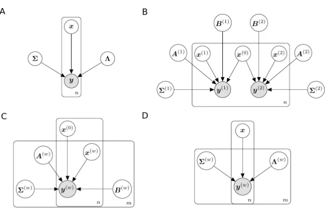
whereyi ∈Rp×1 is modeled as a linear transformation of a latent vectorxi ∈Rk×1 through loading matrixΛ∈Rp×k(Figure 1A). Here,x
iis assumed to follow aNk(0,Ik) distribution,
whereIkis thek-dimensional identity matrix, andi ∼ Np(0,Σ), whereΣis ap×pdiagonal
matrix. With an isotropic noise assumption, Σ = Iσ2, this model has a probabilistic
principal components analysis interpretation (Roweis, 1998; Tipping and Bishop, 1999b). For factor analysis, and in this work, it is assumed thatΣ= diag(σ12,· · · , σp2) representing independent idiosyncratic noise (Tipping and Bishop, 1999a).
Integrating over the factors xi, we see that the covariance of yi is estimated with a
low-rank matrix factorization: ΛΛT +Σ. We further let Y = [y1, . . .yn] be the collection
Figure 1: Graphical representation of different latent factor models. Panel A: Factor analysis model. Panel B: Bayesian canonical correlation analysis model (BCCA). Panel C: An extension of BCCA model to multiple observations. Panel D: Our Bayesian group factor analysis model (BASS).
analysis model for the observationY is written as
Y =ΛX +E. (2)
2.2 Probabilistic canonical correlation analysis
In the context of two paired observations y(1)i ∈ Rp1×1 and y(2)
i ∈ Rp2
×1 on the same n
samples, canonical correlation analysis (CCA) seeks to find linear projections (canonical directions) such that the sample correlations in the projected space are mutually max-imized (Hotelling, 1936). The work of interpreting CCA as a probabilistic model can be traced back to classical descriptions (Bach and Jordan, 2005). With a common latent factor,
xi∈Rk×1,yi(1) and y (2)
i are modeled as
y(1)i =Λ(1)xi+e(1)i ,
y(2)i =Λ(2)xi+e(2)i . (3)
In this model, the errors are distributed as e(1)i ∼ Np1(0,Ψ
(1)) and e(2)
i ∼ Np2(0,Ψ
(2)),
2.3 Bayesian CCA with group-wise sparsity
Building on the probabilistic CCA model, a Bayesian CCA (BCCA) model has the following form (Klami et al., 2013)
yi(1)=A(1)x(0)i +B(1)x(1)i +(1)i ,
yi(2)=A(2)x(0)i +B(2)x(2)i +(2)i , (4) with x(0)i ∈ Rk0×1, x(1)i ∈ Rk1×1 and x
(2)
i ∈ Rk2×1 (Figure 1B). The latent vector x (0) i is
shared by bothyi(1)andy(2)i , and captures their common variation through loading matrices
A(1) andA(2). Two additional latent vectors,x(1)i andx(2)i , are specific to each observation; they are multiplied by observation-specific loading matricesB(1)andB(2). The two residual error terms are(1)i ∼ Np1(0,Σ
(1)) and(2)
i ∼ Np2(0,Σ
(2)), whereΣ(1)andΣ(2)are diagonal
matrices. This model was originally called inter-battery factor analysis (IBFA) (Browne, 1979) and recently has been studied under a full Bayesian inference framework (Klami et al., 2013). It may be interpreted as the probabilistic CCA model (Equation 3) with an additional low-rank factorization of the observation-specific error covariance matrices. In particular, we re-write the residual error term specific to observation w (w = 1,2) from the probabilistic CCA model (Equation 3) as e(iw) = B(w)x(iw) +(iw); then marginally
e(iw) ∼ Npw(0,Ψ
(w)) whereΨ(w) =B(w)(B(w))T +Σ(w).
Recent work has re-written the BCCA model as a factor analysis model with group-wise sparsity in the loading matrix (Klami et al., 2013). Letyi ∈Rp×1 (where p=p1+p2) be
the vertical concatenation of y(1)i and yi(2); let xi ∈Rk×1 (where k=k0+k1+k2) be the
vertical concatenation ofx(0)i ,x(1)i andx(2)i ; and leti ∈Rp×1 be the vertical concatenation of the two residual errors. Then, the BCCA model (Equation 4) may be written as a factor analysis model
yi =Λxi+i,
withi ∼Np(0,Σ), where
Λ=
A(1) B(1) 0 A(2) 0 B(2)
, Σ=
Σ(1) 0 0 Σ(2)
.
The structure in the loading matrix Λ has a specific meaning: the non-zero columns (i.e.,
A(1) andA(2)) project the shared latent factors (i.e., the firstk0elements ofxi) toyi(1) and y(2)i , respectively; these latent factors represent the covariance shared across the observa-tions. The columns with zero blocks (i.e., [B(1);0] or [0;B(2)]) relate factors to only one of the two observations; they model covariance specific to that observation. Under this model, the block sparse structure of Λis imposed via observation-wise sparsity on each factor.
2.4 Extensions to multiple observations
Chen, 2011; Ray et al., 2014). Generally, these approaches partition the latent variables into those that are shared and those that are observation-specific as follows:
y(iw)=A(w)x(0)i +B(w)x(iw)+(iw) for w= 1, . . . , m.
By vertical concatenation of yi(w), xi(w) and (iw), this model can be viewed as a latent factor model (Equation 1) with the joint loading matrix Λ having a similar observation-wise sparsity pattern as the BCCA model
Λ=
A(1) B(1) · · · 0 A(2) 0 · · · 0
..
. ... . .. ...
A(m) 0 · · · B(m)
. (5)
Here, the first column of blocks (A(w)) is a non-zero loading matrix across the features of all observations; the remaining columns have a block diagonal structure with observation-specific loading matrices (B(w)) on the diagonal. However, those extensions are limited by the strict diagonal structure of the loading matrix. Structuring the loading matrix in this way prevents this model from capturing covariance structure among arbitrary subsets of observations. On the other hand, there are an exponential number of possible subsets of observations, making estimation of covariance structure among all observation subsets intractable for largem.
The structure onΛin Equation (5) has been relaxed to model covariance among subsets of the observations (Jia et al., 2010; Virtanen et al., 2012; Klami et al., 2014b). In the relaxed formulation, each observation y(iw) is modeled by its own loading matrix Λ(w) and a shared latent vector xi (Figure 1D):
yi(w)=Λ(w)xi+(iw) for w= 1, . . . , m. (6)
By allowing columns in Λ(w) to be zero, the model decouples certain latent factors from certain observations. The covariance structure of an arbitrary subset of observations is modeled by factors with non-zero loading columns corresponding to the observations in that subset. Factors that correspond to non-zero entries for only one observation capture covariance specific to that observation. Two different approaches have been proposed to achieve column-wise shrinkage in this framework: Bayesian shrinkage (Virtanen et al., 2012; Klami et al., 2014b) and explicit penalties (Jia et al., 2010). The group factor analysis (GFA) model puts an ARD prior (Tipping, 2001) on the loading column for each observation to allow column-wise shrinkage (Virtanen et al., 2012; Klami et al., 2014b):
λ(jhw)∼ N
0,α(hw)−1
for j= 1, . . . , pw,
α(hw)∼Ga(a0, b0),
parameter α(hw) to have large values or values near zero, either pushing elements of λ(·hw)
toward zero or imposing minimal shrinkage, and enabling observation-specific, column-wise sparsity.
Other work puts alternative structured regularizers onΛ(w) (Jia et al., 2010). To induce observation-specific, column-wise sparsity, GFA used mixed norms: an `1 norm penalizes
each observation-specific column, and either `2 or `∞ norms penalize the elements in an
observation-specific column:
φ(Λ(w)) =
k
X
h=1
||λ(·hw)||2 or φ(Λ(w)) =
k
X
h=1
||λ(·hw)||∞.
The `1 norm penalty achieves observation-specific column-wise shrinkage. Both of these
mixed-norm penalties create a bi-convex problem in Λand X.
These two approaches of adaptive structured regularization in GFA models capture covariance uniquely shared among arbitrary subsets of the observations and avoid mod-eling shared covariance in non-maximal subsets. But neither the ARD approach nor the mixed-norm penalties encourages element-wise sparsity within loading columns. Adding element-wise sparsity is important because it results in interpretable latent factors, where features with non-zero loadings in a specific factor have an interpretation as a cluster (West, 2003; Carvalho et al., 2008). To induce element-wise sparsity, one can either use Bayesian shrinkage on each loading (Carvalho et al., 2010) or a mixed norm with `1 type penalties
on each element (i.e.,Pk
h=1
Pp
j=1|λ (w) jh |).
A more recent GFA model is a step toward both column-wise and element-wise spar-sity (Khan et al., 2014). In this model, element-wise sparspar-sity is achieved by putting inde-pendent ARD priors on each loading element, and column-wise sparsity is achieved by a spike-and-slab prior on the loading columns. However, ARD priors do not allow the model to adjust shrinkage levels within each factor, and this approach does not include sparse and dense factors. One contribution of our work is to define a carefully structured Bayesian shrinkage prior on the loading matrix of a GFA model that encourages both element-wise and column-wise shrinkage, and that includes both sparse and dense factors.
3. Bayesian structured sparsity
3.1 Bayesian sparsity-inducing priors
Bayesian shrinkage priors have been widely used in latent factor models due to their flexi-ble and interpretaflexi-ble solutions (West, 2003; Carvalho et al., 2008; Polson and Scott, 2011; Knowles and Ghahramani, 2011; Bhattacharya and Dunson, 2011). In Bayesian statistics, a regularizing term,φ(Λ), may be viewed as a marginal prior proportional to exp(−φ(Λ)); the regularized optimum then becomes the maximum a posteriori (MAP) solution (Polson and Scott, 2011). For example, the well known `2 penalty for coefficients in linear
regres-sion models corresponds to Gaussian priors, also known as ridge regresregres-sion or Tikhonov regularization (Hoerl and Kennard, 1970). In contrast, an`1 penalty corresponds to double
exponential or Laplace priors, also known as the Bayesian Lasso (Tibshirani, 1996; Park and Casella, 2008; Hans, 2009).
When the goal of regularization is to induce sparsity, the prior distribution should be chosen so that it has substantial probability mass around zero, which draws small effects toward zero, and heavy tails, which allows large signals to escape from substantial shrink-age (O’Hagan, 1979; Carvalho et al., 2010; Armagan et al., 2011). The canonical Bayesian sparsity-inducing prior is the spike-and-slab prior, which is a mixture of a point mass at zero and a flat distribution across the space of real values, often modeled as a Gaussian with a large variance term (Mitchell and Beauchamp, 1988; West, 2003). The spike-and-slab prior has elegant interpretability by estimating the probability that certain loadings are excluded, modeled by the ‘spike’ distribution, or included, modeled by the ‘slab’ distribution (Car-valho et al., 2008). This interpretability comes at the cost of having exponentially many possible configurations of model inclusion parameters in the loading matrix.
Recently, scale mixtures of normal priors have been proposed as a computationally efficient alternative to the two component spike-and-slab prior (West, 1987; Carvalho et al., 2010; Polson and Scott, 2011; Armagan et al., 2013, 2011; Bhattacharya et al., 2014). Such priors generally assume normal distributions with a mixed variance term. The mixing distribution of the variance allows strong shrinkage near zero but weak regularization away from zero. For example, an inverse gamma distribution on the variance term results in an ARD prior (Tipping, 2001), and an exponential distribution on the variance term results in a Laplace prior (Park and Casella, 2008). The horseshoe prior, with a half Cauchy distribution on the standard deviation as the mixing density, has become popular due to its strong shrinkage and heavy tails (Carvalho et al., 2010).
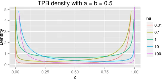
Figure 2: Density of the three parameter beta (T PB) distribution with different values of ν. Five different values ofν ={0.01,0.1,1,10,100}for the three parameter beta distribution with a =b = 0.5. The x-axis represents the value of random variable z, and the y-axis represents the density of random variablez.
3.2 Three parameter beta prior
The three parameter beta (T PB) distribution for a random variable Z ∈ (0,1) has the following density (Armagan et al., 2011):
f(z;a, b, ν) = Γ(a+b) Γ(a)Γ(b)ν
bzb−1(1−z)a−1{1 + (ν−1)z}−(a+b), (7)
where a, b, φ > 0. We denote this distribution as T PB(a, b, ν). When 0 < a < 1 and 0 < b < 1, the distribution is bimodal, with modes at 0 and 1 (Figure 2). The variance parameter ν gives the distribution freedom: with fixed a and b, smaller values of ν put greater probability on z = 1, while larger values of ν move the probability mass towards z= 0 (Armagan et al., 2011). Withν = 1, this distribution is identical to a beta distribution (i.e.,Be(b, a)).
Let λdenote the parameter to which we are applying sparsity-inducing regularization. We assign the following T PBnormal scale mixture distribution, T PBN, toλ:
λ|ϕ∼ N
0,1
ϕ−1
, with ϕ∼ T PB(a, b, ν),
where theshrinkage parameter ϕfollows aT PBdistribution. Witha=b= 1/2 andν = 1, this prior becomes the horseshoe prior (Carvalho et al., 2010; Armagan et al., 2011; Gao et al., 2013). The bimodal property ofϕinduces two distinct shrinkage behaviors: the mode near one encourages ϕ1 −1 towards zero and induces strong shrinkage onλ; the mode near zero encourages ϕ1 −1 large, creating a diffuse prior onλ. Further decreasing the variance parameterν supports stronger shrinkage (Armagan et al., 2011; Gao et al., 2013). If we let θ= ϕ1 −1, then this mixture has the following hierarchical representation:
Note the difference between the ARD prior and the T PB: the ARD prior induces sparsity using an inverse gamma prior on θ, whereas theT PB induces sparsity by using a gamma prior on the θ variable and then regularizing the rate parameter δ using a second gamma prior. These differences lead to different behavior of ARD and theT PB in theory (Polson and Scott, 2011) and in practice, as we show below.
3.3 Global-factor-local shrinkage
The flexible representation of the T PB prior makes it an ideal choice for latent factor models. Our recent work extended the T PB prior to three levels of regularization on a loading matrix (Gao et al., 2013):
%∼ T PB(e, f, ν), (Global)
ζh ∼ T PB
c, d,1
% −1
, (Factor-specific)
ϕjh ∼ T PB
a, b, 1
ζh −1
, (Local)
λjh ∼ N
0, 1
ϕjh −1
. (8)
At each of the three levels, a T PBdistribution is used to induce sparsity via its estimated variance parameter (νin Equation 7), which in turn is regularized using aT PBdistribution. Specifically, the global shrinkage parameter% applies strong shrinkage across thekcolumns of the loading matrix and jointly adjusts the support of column-specific parameter ζh,h∈ {1, . . . , k}close to either zero or one. This can be interpreted as inducing sufficient shrinkage across loading columns to recover the number of factors supported by the observed data. In particular, when ζh is close to one, all elements of columnh are close to zero, effectively
removing thehth component. When near zero, the factor-specific regularization parameter ζh adjusts the shrinkage applied to each element of the hth loading column, estimating
the column-wise shrinkage by borrowing strength across all elements (i.e., features) in that column. The local shrinkage parameter, ϕjh, creates element-wise sparsity in the loading
matrix through a T PBN. Three levels of shrinkage allow us to model both column-wise and element-wise shrinkage simultaneously, and give the model nonparametric behavior in the number of factors via model selection.
Equivalently, this global-factor-local shrinkage prior can be written as (Armagan et al., 2011; Gao et al., 2013):
Global (
γ ∼Ga(f, ν), η∼Ga(e, γ)),
Factor-specific (
τh ∼Ga(d, η),
φh ∼Ga(c, τh),
Local (
δjh∼Ga(b, φh),
θjh ∼Ga(a, δjh),
We further extend our prior to jointly model sparse and dense components by assigning to the local shrinkage parameter a two-component mixture distribution (Gao et al., 2013):
θjh ∼πGa(a, δjh) + (1−π)δφh(·), (10)
where δφh(·) is the Dirac delta function centered atφh. The motivation for this two
com-ponent mixture is that, in real applications such as the analysis of gene expression data, it has been shown that much of the variation in the observation is due to technical (e.g., batch, platform) or biological effects (e.g., sex, ethnicity), which impact a large number of features (Leek et al., 2010). Therefore, loadings corresponding to these effects will often not be sparse. A two-component mixture (Equation 10) allows the prior on the loading (Equation 8) to select between element-wise sparsity or column-wise sparsity. Element-wise sparsity is encouraged via the T PBN prior. Column-wise sparsity jointly regularizes each element of the column with a shared variance term: λjh ∼ N
0,ζ1
h −1
. Modeling each element in a column using a shared regularized variance term has two possible behaviors: i)ζh in Equation (8) is close to 1 and the entire column is shrunk towards zero, effectively
removing this factor; ii) ζh is close to zero, and all elements of the column have a shared
Gaussian distribution, inducing only non-zero elements in that loading. We call included factors that have only non-zero elements dense factors.
Jointly modeling sparse and dense factors effectively combines low-rank covariance fac-torization with interpretability (Zou et al., 2006; Parkhomenko et al., 2009). The dense factors capture the broad effects of observation confounders, model a low-rank approxi-mation of the covariance matrix, and usually account for a large proportion of variance explained (Chandrasekaran et al., 2011). The sparse factors, on the other hand, capture the small groups of interacting features in a (possibly) high-dimensional sparse space, and usually account for a small proportion of the variance explained.
We introduce indicator variables zh,h= 1, . . . , k, to indicate which mixture component
each θjh is generated from in Equation (10), where zh = 1 means θjh ∼ Ga(a, δjh) and
zh = 0 means θjh ∼δφh(·). Thus, a component is a sparse factor when zh = 1 and either
a dense factor or eliminated when zh = 0. We let z = [z1, . . . , zk] and put a Bernoulli
distribution with parameterπ onzh. We further letπhave a flat beta distributionBe(1,1).
This construct allows us to quantify the posterior probability that each factorhis generated from each mixture component type viazh.
4. Bayesian group factor analysis with structured sparsity
that include no observations in the associated loading column are removed from the model. We refer to this model as Bayesian group factor Analysis with Structured Sparsity (BASS). We summarize BASS as follows. The generative model for mcoupled observationsyi(w)
withw= 1, . . . , m andi= 1, . . . , n is
y(iw)=Λ(w)xi+(iw), for w= 1, . . . , m.
This model is written as a latent factor model by concatenating them feature vectors into vectoryi
yi =Λxi+i,
xi ∼ Nk(0,Ik),
i ∼ Np(0,Σ), (11)
where Σ = diag(σ12, . . . , σ2p) and p = Pm
w=1pw. We put independent global-factor-local T PBpriors (Equation 9) on Λ(w):
Global (
γ(w)∼Ga(f, ν), η(w) ∼Ga(e, γ(w))), Factor-specific
(
τh(w)∼Ga(d, η(w)), φ(hw) ∼Ga(c, τh(w)), Local
(
δ(jhw)∼Ga(b, φ(hw)), θ(jhw)∼Ga(a, δjh(w)), λ(jhw)∼ N(0, θ(jhw)). We allow local shrinkage to follow a two-component mixture
θjh(w)∼π(w)Ga(a, δjh(w)) + (1−π(w))δ
φ(w)h (·),
where the mixture proportion has a beta distribution
π(w)∼Be(1,1).
We put a conjugate inverse gamma distribution on the residual variance parameters
σ−2j ∼Ga(aσ, bσ).
In our application of BASS, we set the hyperparameters of the global-factor-local T PB
prior to a = b = c = d = e = f = 0.5, which recapitulates the horseshoe prior at all three levels of the hierarchy. The hyperparameters for the error variances,aσ and bσ, were
5. Parameter estimation
Given our setup, the full joint distribution of the BASS model factorizes as
p(Y,X,Λ,Θ,∆,Φ,T,η,γ,Z,Σ,π)
=p(Y|Λ,X,Σ)p(X)
×p(Λ|Θ)p(Θ|∆,Z,Φ)p(∆|Φ)p(Φ|T)p(T|η)p(η|γ)
×p(Σ)p(Z|π)p(π),
where Θ={θ(jhw)},∆= {δjh(w)}, Φ={φ(hw)}, T ={τh(w)},η = {η(w)} and γ ={γ(w)} are the collections of the global-factor-localT PBprior parameters. The posterior distributions of model parameters may be either simulated through Markov chain Monte Carlo (MCMC) methods or approximated using variational Bayes approaches. We derive an MCMC al-gorithm based on a Gibbs sampler (Appendix A). The MCMC alal-gorithm updates the joint loading matrix row by row using block updates, enabling relatively fast mixing (Bhat-tacharya and Dunson, 2011).
In many applications, we are interested in a single point estimate of the parameters instead of the complete posterior estimate; thus, often an expectation maximization (EM) algorithm is used to find amaximum a posteriori(MAP) estimate of model parameters using conjungate gradient optimization (Dempster et al., 1977). In EM, the latent factorsX and the indicator variables Z are treated as missing data and their expectations estimated in the E-step conditioned on the current values of the parameters; then the model parameters are optimized in the M-step conditioning on the current expectations of the latent variables. Let Ξ = {Λ,Θ,∆,Φ,T,η,γ,π,Σ} be the collection of the parameters optimized in the M-step. The expected complete log likelihood, denoted Q(·), may be written as
Q(Ξ|Ξ(s)) =EX,Z|Ξ(s),Y [log (p(Ξ,X,Z|Y))].
Since X and Z are conditionally independent givenΞ, the expectation may be calculated using the full conditional distributions ofX and Z derived for the MCMC algorithm. The derivation of the EM algorithm for BASS is then straightforward (Appendix B); note that, when estimating Λ, the loading columns specific to each observation are estimated jointly.
5.1 Identifiability
In the BASS model, we have rotational invariance when we right multiply the joint loading matrix by PT and left multiply xby P, producing an identical covariance matrix and likelihood. This rotation invariance is addressed in BASS because the non-sparse ro-tations of the loading matrix violates the prior structure induced by the observation-wise and element-wise sparsity.
Scale invariance is a second identifiability problem inherent in latent factor models. In particular, scale invariance means that a loading can be multiplied by a non-zero constant and the corresponding factor by the inverse of that constant, and this will result in the same data likelihood. This problem we and others have addressed satisfactorily by using posterior probabilities as optimization objectives instead of likelihoods and by including regularizing priors on the factors that restrict the magnitude of the constant. We make an effort to not interpret the relative or absolute scale of the factors or loadings including sign beyond setting a reasonable threshold for zero.
Finally, factor analysis is identifiable up to label switching, or shuffling theh= 1, . . . , k indices of the loadings and factors, assuming we do not take the lower triangular approach. Other approaches put distributions on the loading sparsity or proportion of variance plained in order to address this problem (Bhattacharya and Dunson, 2011). We do not ex-plicitly order or interpret the order of the factors, so we do not address this non-identifiability in the model. Label switching is handled here and elsewhere by a post-processing step, such as ordering factors according to proportion of variance explained. In our simulation studies, we interpret results with this non-identifiability in mind.
5.2 Sparse rotations via PX-EM
Another general problem with latent factor models, including BASS, is the convergence to local optima and sensitivity to parameter initializations. Once the model parameters are initialized, the EM algorithm may be stuck in locally optimal but globally suboptimal regions with undesirable factor orientations. To address this problem, we take advantage of the rotational invariance of the factor analysis framework. Parameter expansion (PX) has been shown to reduce the initialization dependence by introducing auxiliary variables that rotate the current estimate of the loading matrix to best respect the prior while keeping the likelihood stable (Liu et al., 1998; Dyk and Meng, 2001).
We extend our model (Equation 11) using parameter expansion R, a positive definite k×k matrix, as
yi =ΛR−1L xi+i,
xi ∼ Nk(0,R),
i ∼ Nk(0,Σ),
whereRLis the lower triangular matrix of the Cholesky decomposition ofR. The covariance
of yi is invariant under this expansion, and, correspondingly, the likelihood is stable. Note R−1L is not an orthogonal matrix; however, because it is full rank, it can be transformed into an orthogonal matrix times a rotation matrix via a polar decomposition (Rockov´a and George, 2015). We let Λ? = ΛR−1L and assign our BASS T PBN prior to this rotated
We let Ξ? = {Λ?,Θ,∆,Φ,T,η,γ,π,Σ}, and the parameters of our expanded model are {Ξ?∪R}. The EM algorithm in this expanded parameter space generates a sequence of parameter estimates{Ξ?(1)∪R(1),Ξ?(2)∪R(2), . . .}, which corresponds to a sequence of
parameter estimates in the original space {Ξ(1),Ξ(2), . . .}, where Λis recovered via Λ?RL
(Rockov´a and George, 2015). We initializeR(0)=Ik. The expected complete log likelihood
of this PX BASS model is
Q(Ξ?,R|Ξ(s)) =EX,Z|Ξ(s),Y,R0log p(Ξ
?,R,X,Z|Y)
. (12)
In our parameter-expanded EM (PX-EM) for BASS, the conditional distributions of
X and Z still factorize in the expectation. However, the distribution of xi depends on
expansion parameter R. The full joint distribution (Equation 11) has a single change in p(X), with Λ? in the place ofΛ. In the M-step, theR that maximizes Equation (12) is
R(s)= arg max
R
Q(Ξ?,R|Ξ(s)) = arg max
R
const− n
2 log|R| − 1 2tr R
−1SXX
,
where SXX = Pn
i=1hx·ixT·ii. The solution is R(s) = n1SXX. For the E-step, Λ is first
calculated and the expectation is taken in the original space (details in Appendix C). Note that the proposed PX-EM for the BASS model keeps the likelihood invariant but does not keep the prior invariant after transformation ofΛ. This is different from the earlier PX-EM algorithm (Liu et al., 1998), as discussed in recent work (Rockov´a and George, 2015). Because the resulting posterior is not invariant, we run PX-EM only for a few iterations and then switch to the EM algorithm. The effect is that the BASS model is substantially less sensitive to initialization (see simulation results). By introducing expansion parameter
R, the posterior modes in the original space are intersected with equal likelihood curves indexed byRin expanded space. Those curves facilitate traversal between posterior modes in the original space and encourage initial parameter estimates with appropriate sparse structure in the loading matrix (Rockov´a and George, 2015).
5.3 Computational complexity
The computational complexity of the block Gibbs sampler for the BASS model is demand-ing. Updating each loading row requires the inversion of a k×k matrix with O(k3) com-plexity and then calculating means with O(k2n) complexity. The complexity of updating the full loading matrix repeats this calculation p times. Other updates are of lower order relative to updating the loading. Our Gibbs sampler has O(k3p+k2pn) complexity per iteration, which makes MCMC difficult to apply when pis large.
In the BASS EM algorithm, the E-step has complexity O(k3) for a matrix inversion, complexityO(k2p+kpn) for calculating the first moment, and complexity O(k2n) for cal-culating the second moment. Calculations in the M-step are all of a lower order. Thus, the EM algorithm has complexity O(k3+k2p+k2n+kpn) per iteration.
6. Simulations and comparisons
We demonstrate the performance of our model on simulated data in three settings: paired observations, four observations, and ten observations.
6.1 Simulations
We describe the details of the three types of simulations here.
6.1.1 Simulations with paired observations (CCA)
We simulated two data sets with p1 = 100, p2 = 120 in order to compare results from our
method to results from state-of-the-art CCA methods. The number of samples in these simulations was n = {20,30,40,50}, chosen to be smaller than both p1 and p2 to reflect
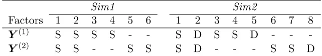
the large p, small n regime (West, 2003) that motivated our structured approach. We first simulated observations with only sparse latent factors (Sim1). In particular, we set k = 6, where two sparse factors are shared by both observations (factors 1 and 2; Table 1), two sparse factors are specific toy(1) (factors 3 and 4; Table 1), and two sparse factors
are specific to y(2) (factors 5 and 6; Table 1). The elements in the sparse loading matrix were randomly generated from a N(0,4) Gaussian distribution, and sparsity was induced by setting 90% of the elements in each loading column to zero at random (Figure 3A). We zeroed values of the sparse loadings for which the absolute values were less than 0.5. Latent factors x were generated fromN6(0,I6). Residual error was generated by first generating
thep=p1+p2 diagonals on the residual covariance matrixΣfrom a uniform distribution
on (0.5,1.5), and then generating each column of the error matrix from Np(0,Σ).
We performed a second simulation that included both sparse and dense latent factors (Sim2). In particular, we extended Sim1 tok= 8 latent factors, where one of the shared sparse factors is now dense, and two dense factors, each specific to one observation, were added. For all dense factors, each loading was generated according to a N(0,4) Gaussian distribution (Table 1; Figure 3B).
Sim1 Sim2
Factors 1 2 3 4 5 6 1 2 3 4 5 6 7 8
Y(1) S S S S - - S D S S D - -
-Y(2) S S - - S S S D - - - S S D
Table 1: Latent factors in Sim1 and Sim2 with two observation matrices. S represents a sparse vector; D represents a dense vector; - represents no contribution to that observation from the factor.
6.1.2 Simulations with four observations (GFA)
We performed two simulations (Sim3 and Sim4) including four observations with p1 =
Sim3 Sim4
Factors 1 2 3 4 5 6 1 2 3 4 5 6 7 8
Y(1) S - - S - - S - - - D - -
-Y(2) - S - S S S - S - S - D -
-Y(3) - - S - S S - - S S - - D
-Y(4) - - - S - - S - - - - D
Table 2: Latent factors in Sim3 and Sim4 with four observation matrices. S represents a sparse vector; D represents a dense vector; - represents no contribution to that observation from the factor.
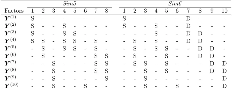
Sim5 Sim6
Factors 1 2 3 4 5 6 7 8 1 2 3 4 5 6 7 8 9 10
Y(1) S - - - S - - - D - - -Y(2) S - - S - - - - S - - S - - D - -
-Y(3) S - - S S - - - - - - S - - D D -
-Y(4) S S - S S - S - - S - S - - D D - -Y(5) - S - S S - S - - S - S S - - D D
-Y(6) - S - - - - S S - S - - S - - D D
-Y(7) - - S - - - S S - S S - S - - - D D Y(8) - - S - - - S S - - S - S - - - D D
Y(9) - - S - - - - S - - S - - - - - - D
Y(10) - - S - - S - - - - S - - S - - - D
Table 3: Latent factors in Sim5 and Sim6 with four observation matrices. S represents a sparse vector; D represents a dense vector; - represents no contribution to that observation from the factor.
included both sparse and dense factors (Table 2). Samples from these two simulations were generated following the same procedure as the simulations with two observations.
6.1.3 Simulations with ten observations (GFA)
To further evaluate BASS on multiple observations, we performed two additional simulations (Sim5 and Sim6) on ten coupled observations withpw= 50 forw= 1, . . . ,10. The number
of samples was set to n={20,30,40,50}. InSim5, we let k= 8 and only simulated sparse factors (Table 3). In Sim6 we let k = 10 and simulated both sparse and dense factors (Table 3). Samples in these two simulations were generated following the same method as in the simulations with two observations.
6.2 Methods for comparison
analysis (JFA) (Ray et al., 2014). We also included the linear version of a flexible non-linear model, manifold relevance determination (MRD) (Damianou et al., 2012). To evaluate the sensitivity of BASS to initialization, we compared three different initialization methods: random initialization (EM), 50 iterations of MCMC (MCMC-EM), and 20 iterations of PX-EM (PX-EM); each of these were followed with EM until convergence, reached when both the number of non-zero loadings do not change for titerations and the log likelihood changes<1×10⁻⁵ within titerations. We performed 20 runs for each version of inference in BASS: EM, MCMC-EM, and PX-EM. In Sim1 and Sim3, we set the initial number of factors to k= 10. In Sim2, Sim4,Sim5, and Sim6, we set the initial number of factors to 15.
The GFA model (Klami et al., 2013) uses an ARD prior to encourage column-wise shrinkage of the loading matrix, but not sparsity within the loadings. The computational complexity of this GFA model with variational updates is O(k3m+k2p+k2n+kpn) per iteration, which is nearly identical to BASS but includes an additional factorm, the number of observations, scaling the k3 term. In our simulations, we ran the GFA model with the factor number set to the correct value.
The sGFA model (Khan et al., 2014) encourages element-wise sparsity using independent ARD priors on loading elements. Loading columns are modeled with a spike-and-slab type mixture to encourage column-wise sparsity. Inference is performed with a Gibbs sampler without using block updates. Its complexity is O(k3+k2pn) per iteration, which, whenk is large, will dominate the per-iteration complexity of BASS; furthermore, Gibbs samplers typically require greater numbers of iterations than EM-based methods. We ran the sGFA model with the correct number of factors in our six simulations.
We ran the regularized version of classical CCA (RCCA) for comparison in Sim1 and
Sim2 (Gonz´alez et al., 2008). Classical CCA tries to find kcanonical projection directions
uh andvh (h= 1, . . . , k) forY(1) andY(2)respectively such that i) the correlation between uThY(1) and vhTY(2) is maximized forh= 1, . . . , k; and ii)uTh0Y(1) is orthogonal to uThY(1)
with h0 6=h, and similarly for vh and Y(2). Let these two projection matrices be denoted U = [u1, . . . ,uk]∈Rp1×k and V = [v1, . . . ,vk]∈Rp2×k. These matrices are the maximum likelihood estimates of the shared loading matrices in the Bayesian CCA model up to or-thogonal transformations (Bach and Jordan, 2005). However, classical CCA requires the observation covariance matrices to be non-singular and thus is not applicable in the current simulations wheren < p1, p2.
Here, we used a regularized version of CCA (RCCA) (Gonz´alez et al., 2008), which regularizes CCA using an `2-type penalty by adding λ1Ip1 and λ2Ip2 to the two sample
covariance matrices. The effect of this penalty is not to induce sparsity but instead to allow application topn data sets. The two regularization parameters (λ1 and λ2) were
chosen according to leave-one-out cross-validation with the search space defined on a 11×11 grid from 0.0001 to 0.01. The projection directionsU andV were estimated using the best regularization parameters. We letΛ0= [U;V]; this matrix was comparable to the simulated loading matrix up to orthogonal transformations. We calculated the matrixP such that the Frobenius norm between Λ0PT and simulated Λ was minimized, with the constraint that
6 and 8 in Sim1 and Sim2, respectively, representing the true number of latent factors. RCCA does not apply to multiple coupled observations, and therefore it was not included in further simulations.
The sparse CCA (SCCA) method (Witten and Tibshirani, 2009) maximizes correlation between two observations after projecting the original space with a sparsity-inducing penalty onto the latent components, producing sparse matrices U and V. This method is encoded in the R packagePMA(Witten et al., 2013). ForSim1 andSim2, as with RCCA, we found an optimal orthogonal transformation matrixP such that the Frobenius norm betweenΛSPT
and simulated Λwas minimized, whereΛS was the vertical concatenation of the recovered
sparse U and V. We chose 6 and 8 sparse projections in Sim1 and Sim2, respectively, representing the true number of linear factors. Because both RCCA and SCCA are both deterministic and greedy, the results fork <6 are all implicitly available by subsetting the factors in the k= 6 results.
An extension of SCCA allows for multiple observations (Witten and Tibshirani, 2009). For Sim3 and Sim4, we recovered four sparse projection matrices U(1),U(2),U(3),U(4), and for Sim5 and Sim6, we recovered ten projection matrices. ΛS was calculated with the
concatenation of those projection matrices. Then the orthogonal transformation matrix P
was calculated similarly by minimizing the Frobenius norm between ΛSPT and the true
loading matrix Λ. The number of canonical projections was set to 6 in Sim3, 8 in Sim4
and Sim5, and 10 in Sim6, corresponding to the true number of latent factors.
The Bayesian joint factor analysis model (JFA) (Ray et al., 2014) puts an Indian buffet process (IBP) prior (Griffiths and Ghahramani, 2011) on the factors, inducing element-wise sparsity, and an ARD prior on the variance of the loadings. The idea of putting an IBP on a latent factor model, which gives desirable nonparametric behavior in the number of latent factors and also produces element-wise sparsity in the loading matrix, was described for the Nonparametric Sparse Factor Analysis (NSFA) model (Knowles and Ghahramani, 2011). Similarly, in JFA, element-wise sparsity is encouraged both in the factors and in the loadings. JFA partitions latent factors into a fixed number of observation-specific factors and factors shared by all observations, and does not include column-wise sparsity. Its complexity is O(k3+k2pn) per iteration of the Gibbs sampler. We ran JFA on our simulations with the number of factors set to the correct values. Because the JFA model uses a sparsity-inducing prior instead of an independent Gaussian prior on the latent factors, the resulting model does not have a closed form posterior predictive distribution (Equation 13); therefore, we excluded the JFA model from prediction results.
used the linear version of this model for a fair comparison. We ran the MRD model on our simulated data with the correct number of factors.
We summarize the parameter choices for all methods here:
sGFA: We used the getDefaultOpts function in the sGFA package to set the default pa-rameters. In particular, the ARD prior was set to Ga(10−3,10−3). The prior on the inclusion probabilities was set to beta(1,1). Total MCMC iterations were set to 105 withsampling iterations set to 1,000 and thinning stepsset to 5.
GFA: We used the getDefaultOpts() function in the GFA package to set the default pa-rameters. In particular, the ARD prior for both loading and error variance was set to Ga(10−14,10−14). The maximum iteration parameter was set to 105, and the “L-BFGS” optimization method was used.
RCCA: The regularization parameter was chosen using leave-one-out cross-validation on an 11×11 grid from 0.0001 to 0.01 using the functionestim.regulin theCCApackage.
SCCA: We used thePMApackage with Lasso penalty (thetypexandtypezparameters in the functionCCAwere set to “standard”). This corresponds to setting the`1 bound of the
projection vector to 0.3√pw forw= 1,2.
JFA: The ARD priors for both the loading and factor scores were set to Ga(10−5,10−5). The parameters of the beta process prior were set to α = 0.1 and c = 104. The MCMC iterations were set to 1,000 with 200 iterations of burn-in. As is the default settings, we did not thin the chain.
MRD: We used thesvargplvm_initfunction in the GPLVMpackage to initialize parameters. The linar2 kernel was chosen for all observations. Latent variables were initialized by concatenating the observation matrices first (the ‘concatenated’ option) and then performing PCA. Other parameters were set bysvargplvm_initwith default options.
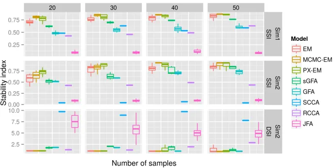
6.3 Metrics for comparison
To compare the results of BASS with the alternative methods, we used the sparse and dense stability indices (Gao et al., 2013) to quantify the distance between the simulated loadings and the recovered loadings. The sparse stability index (SSI) measures the similarity between columns of sparse matrices. SSI is invariant to column scale and label switching, but it penalizes factor splitting and matrix rotation; larger values of SSI indicate better recovery. Let C ∈ Rk1×k2 be the absolute correlation matrix of columns of two sparse
loading matrices. Then SSI is calculated by
SSI = 1 2k1
k1
X
h1=1
max(ch1,·)−
Pk2
h2=1I(ch1,h2 >ch1,·)ch1,h2
k2−1
+ 1
2k2 k2
X
h2=1
max(c·,h2)−
Pk1
h1=1I(ch1,h2 >c·,h2)ch1,h2
k1−1
The dense stability index (DSI) quantifies the difference between dense matrix columns, and is invariant to orthogonal matrix rotation, factor switching, and scale; DSI values closer to zero indicate better recovery. Let M1 and M2 be the dense matrices. DSI is calculated
by
DSI = 1
p2tr(M1M T
1 −M2M2T).
We extended the stability indices to allow multiple coupled observations as in our simu-lations. In Sim1,Sim3, and Sim5, all factors are sparse, and SSIs were calculated between the true sparse loading matrices and recovered sparse loading matrices. InSim2,Sim4, and
Sim6, because none of the methods other than BASS explicitly distinguished sparse and dense factors, we categorized each recovered factor as follows. We first selected a global sparsity threshold on the elements of the combined loading matrix; here we set that value to 0.15. Elements below this threshold were set to zero in the loading matrix. Then we chose the first five loading columns with the fewest non-zero elements as the sparse loadings inSim2, first four such loadings as the sparse loadings inSim4, and first six such loadings as sparse inSim6. The remaining loading columns were considered dense loadings and were not zeroed according to the global sparsity threshold. We found that varying the sparsity threshold did not affect the separation of sparse and dense loadings significantly across methods. SSIs were then calculated for the true sparse loading matrix and the recovered sparse loadings across methods.
To calculate DSIs, we treated the loading matricesΛ(w) for each observation separately, and calculated the DSI for the recovered dense components of each observation. The DSI for each method was the sum of the m separate DSIs. Because the loading matrix is marginalized out in MRD (Lawrence, 2005), we excluded MRD from this comparison.
We further evaluated the prediction performance of BASS and other methods. In the BASS model (Equation 6), the joint distribution of any one observationyi(w) and all other observationsyi(−w) can be written as
yi(w) yi(−w)
!
∼ N
0 0
,
Λ(w)(Λ(w))T +Σ(w) Λ(w)(Λ(−w))T Λ(−w)(Λ(w))T Λ(−w)(Λ(−w))T +Σ(−w)
,
where Λ(−w) and Σ(−w) are the loading matrix and residual covariance excluding the wth observation. Therefore, the conditional distribution of y(iw) is a multivariate response in a multivariate linear regression model, where yi(−w) are the predictors; the mean term takes the form
E(y(iw)|y (−w) i ) =Λ
(w)(Λ(−w))T Λ(−w)(Λ(−w))T +Σ(−w)−1
yi(−w)
=
k
X
h=1
λ(·hw)(λ(−·hw))T Λ(−w)(Λ(−w))T +Σ(−w)−1
yi(−w). (13)
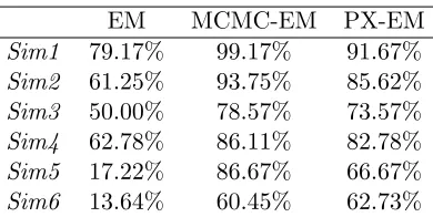
EM MCMC-EM PX-EM
Sim1 79.17% 99.17% 91.67%
Sim2 61.25% 93.75% 85.62%
Sim3 50.00% 78.57% 73.57%
Sim4 62.78% 86.11% 82.78%
Sim5 17.22% 86.67% 66.67%
Sim6 13.64% 60.45% 62.73%
Table 4: Percentage of latent factors correctly identified across 20 runs with n= 40. The columns represent the runs of EM, EM initialized with MCMC (MCMC-EM), and EM initialized with PX-EM.
{10,100,200}. Then, we generated ns = 200 samples as test data using the true model
parameters, simulating the corresponding test data factors X ∼ N(0,1). For each simu-lation study, we chose at least one observation in the test data as the response and used the other observations and model parameters estimated from the training data to perform prediction. Mean squared error (MSE) was used to evaluate the prediction performance. ForSim1 andSim2,yi(2) was the response; forSim3 and Sim4,y(3)i was the response; and forSim5 and Sim6,yi(8),yi(9) and y(10)i were the responses.
6.4 Results of the simulation comparison
We first evaluated the performance of BASS and the other methods in terms of recovering the correct number of sparse and dense factors in the six simulations (Figures S3-S8). We calculated the percentage of correctly identified factors across 20 runs in the simulations withn= 40 (Table 4). Qualitatively, BASS recovered the closest matches to the simulated loading matrices across all methods (Figures 3, S1, S2). The correctly estimated loading matrices by the three different BASS initializations produced similar results; we only plot matrices from the PX-EM method.
6.4.1 Results on simulations with two observations (CCA)
Comparing results with two observations (Sim1 and Sim2), our model produced the best SSIs and DSIs among all methods across all sample sizes (Figures 4). sGFA’s performance was limited for these simulations because the ARD prior does not produce sufficient element-wise sparsity, resulting in low SSIs (Figure 4). As a consequence of not matching sparse loadings well, sGFA had difficulty recovering dense loadings, especially with small sample sizes (Figure 4). GFA had difficulty recovering sparse loadings because of column-wise ARD priors with the same limitation (Figure 3, Figure 4). Its dense loadings were indirectly affected by the lack of sufficient sparsity for small sample sizes (Figure 4). RCCA also had difficulty in the two simulations because the recovered loadings were not sufficiently sparse using the`2-type penalty (Figure 3).
Figure 4: Comparison of stability indices on recovered loading matrices with two observations. Each stability index is plotted across 20 runs. For SSI, a larger value indicates better recovery; for DSI, a smaller value indicates better recovery. The boundaries of the box are the first and third quartiles. The line extends to the highest and lowest observations that are within 1.5 times the distance of the first and third quartiles beyond the box boundaries.
4). Adding dense loadings deteriorated the performance of SCCA (Figures 3B, 4). The JFA model did not recover the true loadings matrix well because of insufficient sparsity in the loadings and additional sparsity in the factors (Figure 3). The SSIs and DSIs for JFA reflect this data-model mismatch (Figure 4).
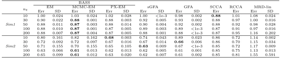
We next evaluated the predictive performance of these methods for two observations. In
Sim1, SCCA achieved the best prediction accuracy in three training sample sizes (Table 5). We attribute this to SCCA recovering well the shared sparse loadings (Figure 3) because the prediction accuracy is only a function of the shared loadings. Note (Equation 13) that zero columns in either Λ(w) orΛ(−w) decouple the contribution of the corresponding factors to the prediction ofyi(w). InSim2, shared sparse and dense factors contribute to the prediction performance, and BASS achieved the best prediction accuracy (Table 5).
6.4.2 Results on simulations with four observations (GFA)
BASS
nt ErrEMSD ErrMCMC-EMSD ErrPX-EMSD ErrsGFASD ErrGFASD SCCAErr RCCAErr ErrMRD-linSD
Sim1
10 1.00 0.024 1.03 0.024 1.02 0.028 1.00 <1e-3 0.98 0.002 0.88 1.01 1.08 0.024 30 0.90 0.022 0.88 0.001 0.88 0.003 0.92 0.005 0.93 0.002 0.88 0.97 1.00 0.016 50 0.88 0.011 0.87 0.003 0.88 0.014 0.90 0.004 0.92 0.002 0.88 0.92 0.98 0.028 100 0.88 0.010 0.87 0.001 0.87 0.005 0.89 0.003 0.89 <1e-3 0.87 0.91 0.97 0.016 200 0.88 0.007 0.87 0.004 0.87 0.005 0.88 0.001 0.88 <1e-3 0.87 0.95 1.16 0.202
Sim2
10 0.80 0.161 0.82 0.162 0.68 0.003 0.74 0.043 0.89 0.023 0.86 0.72 1.14 0.002 30 0.72 0.092 0.72 0.097 0.67 0.016 0.67 0.014 0.66 0.006 0.86 0.70 1.15 0.034 50 0.71 0.155 0.70 0.155 0.65 0.105 0.63 0.009 0.67 <1e-3 0.85 0.72 1.17 0.009 100 0.63 0.066 0.61 0.013 0.62 0.013 0.62 0.005 0.61 0.001 0.85 0.75 1.13 0.013 200 0.65 0.099 0.61 0.012 0.63 0.020 0.62 0.007 0.61 0.002 0.85 0.81 1.55 0.591
Table 5: Prediction accuracy with two observations on ns= 200test samples. Test
samples yi(2) are treated as the response, and training samples y(1)i are used to estimate parameters in order to predict the response. Prediction accuracy is measured by mean squared error (MSE) between simulated y(1)i and E(yi(1)|y
(2)
i ). Values presented are the
mean MSE (Err) and standard deviation (SD) across 20 runs of each method. If SD is missing for a method, then that method was deterministic.
BASS
nt ErrEMSD ErrMCMC-EMSD ErrPX-EMSD ErrsGFASD ErrGFASD SCCAErr ErrMRD-linSD
Sim3
10 1.03 0.044 1.02 0.019 1.01 0.010 1.00 <1e-3 0.97 0.001 1.00 1.00 <1e-3 30 0.91 0.049 0.87 0.016 0.88 0.007 0.90 0.007 0.93 0.003 1.00 0.99 0.021 50 0.85 0.019 0.85 <1e-3 0.87 0.038 0.87 0.005 0.88 0.002 1.01 1.04 0.095 100 0.85 0.019 0.84 0.002 0.84 0.003 0.86 0.004 0.87 0.001 1.11 0.92 0.014 200 0.84 0.001 0.84 <1e-3 0.84 0.004 0.84 0.001 0.83 0.001 1.13 1.16 0.140
Sim4
10 1.05 0.095 1.03 0.094 1.10 0.138 1.00 <1e-3 1.32 0.029 1.35 1.98 0.067 30 0.97 0.020 0.95 0.015 0.96 0.013 0.97 0.007 1.03 0.003 1.40 1.50 0.090 50 0.94 0.013 0.93 0.005 0.94 0.012 0.95 0.005 1.02 0.017 1.40 1.50 0.084 100 0.93 0.015 0.93 0.007 0.93 0.010 0.94 0.003 0.96 <1e-3 1.51 1.47 0.088 200 0.91 0.029 0.92 0.022 0.89 0.047 0.93 0.001 0.89 0.001 1.77 1.58 0.132
Table 6: Prediction accuracy with four observations on ns = 200 test samples.
Test samples yi(3) are treated as the response, and training samples y(1)i , yi(2), and yi(4)
are used to estimate parameters in order to predict the response. Prediction accuracy is measured by mean squared error (MSE) between simulatedy(3)i and E(y(3)i |y
(1) i ,y
(2) i ,y
(4) i ).
Values presented are the mean MSE (Err) and standard deviation (SD) across 20 runs of each method. Standard deviation (SD) is missing for SCCA because the method is deterministic.
MCMC-EM and PX-EM. The advantage of BASS relative to the other methods is apparent in these SSI comparisons, which specifically highlight interpretability and robust recovery of this type of latent structure (Figure 5).
In the context of prediction using four observation matrices, BASS achieved the best prediction performance with y(3)i as the response and the remaining observations as pre-dictors (Table 6). In particular, the MCMC-initialized EM approach had the best overall prediction performance across methods for these two simulations.
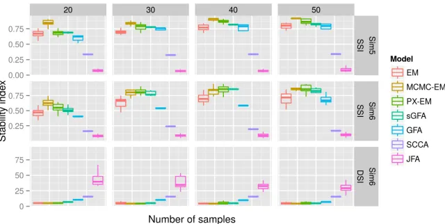
6.4.3 Results on simulations with ten observations (GFA)
Figure 5: Comparison of stability indices on recovered loading matrices with four observations. Each stability index is plotted across 20 runs. For SSI, a larger value indicates better recovery; for DSI, a smaller value indicates better recovery. The boundaries of the box are the first and third quartiles. The line extends to the highest and lowest values that are within 1.5 times the distance of the first and third quartiles beyond the box boundaries.
BASS
nt ErrEMSD ErrMCMC-EMSD ErrPX-EMSD ErrsGFASD ErrGFASD SCCAErr ErrMRD-linSD
Sim5
10 1.01 0.020 1.00 0.011 1.00 0.007 0.99 0.008 1.00 0.002 0.99 1.49 0.001 30 0.88 0.031 0.86 0.018 0.87 0.028 0.89 0.005 0.90 0.002 0.99 1.01 0.035 50 0.86 0.023 0.85 <1e-3 0.86 0.022 0.87 0.003 0.88 0.001 0.99 0.97 0.020 100 0.85 0.007 0.85 <1e-3 0.85 0.002 0.86 0.003 0.87 0.001 1.01 0.92 0.039 200 0.85 0.006 0.84 <1e-3 0.84 <1e-3 0.84 0.001 0.83 0.001 0.96 1.06 0.105
Sim6
10 0.61 0.164 0.57 0.116 0.51 0.031 0.58 0.012 0.75 0.011 0.97 1.00 <1e-3 30 0.49 0.160 0.40 0.093 0.38 0.007 0.43 0.006 0.40 0.005 0.98 0.46 0.006 50 0.44 0.099 0.39 0.011 0.39 0.004 0.41 0.002 0.40 0.001 1.01 0.42 0.009 100 0.39 0.033 0.39 0.004 0.39 0.011 0.39 0.002 0.39 0.001 0.97 0.52 0.249 200 0.38 0.003 0.38 0.001 0.38 0.001 0.39 0.001 0.39 0.001 1.01 0.40 0.020
Table 7: Prediction mean squared error with ten observations on ns = 200 test
samples. Test samples y(8)i ,yi(9) and y(10)i are treated as the response and the rest of the observations are used as the training data to estimate parameters used to predict the response. Prediction accuracy is measured by mean squared error (MSE) between simulated responses and predicted responses. Values presented are the mean MSE (Err) and standard deviation (SD) across 20 runs of each method. Standard deviation (SD) is missing for SCCA because the method is deterministic.
S2). For the stability indices, BASS with MCMC-EM and PX-EM produced the best SSIs inSim5 across all methods and for almost all sample sizes (Figures 6). Here sGFA achieved equal or better SSIs than BASS EM, highlighting the sensitivity of BASS EM to initial-izations. GFA had equivalent or worse SSIs than BASS EM. In this pair of simulations, the advantages of BASS for flexible and robust column-wise and element-wise shrinkage are apparent (Figures 6). BASS also achieved the best prediction performance in Sim5 and
Figure 6: Comparison of stability indices on recovered loading matrices with ten observations. Each stability index is plotted across 20 runs. For SSI, a larger value indicates better recovery; for DSI, a smaller value indicates better recovery. The boundaries of the box are the first and third quartiles. The line extends to the highest and lowest value within 1.5 times the distance of the first and third quartiles beyond the box boundaries.
Across the three BASS methods, MCMC-EM had the most accurate performance across nearly all simulation settings. However, this performance boost comes with the price of running a small number of Gibbs sampling iterations with complexity ofO(k3p+k2pn) per iteration. Whenpis large, even a few iterations are computationally infeasible. PX-EM, on the other hand, has the same complexity as EM, and showed robust and accurate simulation results relative to EM. In the following real applications, we used BASS EM initialized with a small number of iterations of PX-EM.
7. Applying BASS to Mulan Library, genomics data, and text analysis
In this section we considered three real data applications of BASS. In the first application, we evaluated the prediction performance for multiple correlated response variables in the Mulan Library (Tsoumakas et al., 2011). In the second application, we applied BASS to gene expression data from the Cholesterol and Pharmacogenomic (CAP) study. The data consist of expression measurements for about ten thousands genes in 480 lymphoblastoid cell lines (LCLs) under two experimental conditions (Mangravite et al., 2013; Brown et al., 2013). BASS was used to detect sparse covariance structures specific to each experimental condition. In the third application, we applied BASS to approximately 20,000 newsgroup posts to 20 newsgroups (Joachims, 1997) in order to perform multiclass classification.
7.1 Multivariate response prediction: The Mulan Library
(m= 2): the matrix of labels were treated as one observation (Y(1)) and the features were treated as another (Y(2)). Recently Mulan added multiple regression data sets with contin-uous variables. We chose ten benchmark data sets from the Mulan Library. Four of them (bibtex, delicious, mediamill, scene) have binary responses and were studied pre-viously (Klami et al., 2013). Another six data sets (rf1, rf2, scm1d, scm20d, atp1d, atp7d) have continuous responses (Table 8). For all data sets, we removed features with identical values for all samples in the training set as uninformative. For the continuous response data sets, for each value, we subtracted the mean and divided by the standard deviation of each feature.
We ran BASS, sGFA, GFA, and MRD-lin on the ten data sets, and compared the results using prediction accuracy. For data sets with binary labels, we quantified prediction error using the Hamming loss between the predicted labels and true labels. The predicted labels on the test samples were calculated using the same thresholding rules as in earlier work (Klami et al., 2013). The value of the threshold was chosen so that the Hamming loss between the estimated labels and the true labels in the training set was minimized. We used the R packagePresenceAbsenceand Matlab functionperfcurveto find the thresholds to produce binary classifications from continuous predictions. In particular, the R package
PresenceAbsenceselects the threshold by maximizing the percent correctly classified, which corresponds to minimizing the Hamming loss. For continuous variables, mean squared error (MSE) was used to evaluate prediction accuracy. We initialized BASS with 500 factors and 50 PX-EM iterations. The other models were set to the default parameters with the number of factors set to min(p1, p2,50) (see Simulations for details). All methods were run 20 times,
and minimum errors were reported (Tables S1-S11).
BASS achieved the best prediction accuracy in five of the ten data sets (Table 8). For the data sets with a binary response, sGFA produced the best performance compared with other methods, achieving the smallest MSE in all four data sets. GFA had the most stable results in terms of SD in the four data sets. For the continuous response, BASS outperformed the other models in four out of six data sets. GFA again had the most stable MSE compared with other methods. The good performance of BASS on the data sets with continuous response variables may be attributed to the structured sparsity on the loading matrix, achieving the intended gains in generalization error from flexible regularization. Although the ARD prior used in GFA did not produce consistently sparse loadings, this model generated the most stable predictive results.
7.2 Gene expression data analysis