A Practical Scheme and Fast Algorithm to Tune the Lasso With Optimality Guarantees

(1)

A Practical Scheme and Fast Algorithm to

Tune the Lasso With Optimality Guarantees

Micha¨el Chichignoud [email protected]

Seminar for Statistics ETH Z¨urich

Johannes Lederer∗ [email protected]

Department of Statistics and Department of Biostatistics University of Washington

Martin J. Wainwright [email protected]

Department of Statistics

and Department of Electrical Engineering and Computer Sciences University of California at Berkeley

Editor:Francis Bach

Abstract

We introduce a novel scheme for choosing the regularization parameter in high-dimensional linear regression with Lasso. This scheme, inspired by Lepski’s method for bandwidth selec-tion in non-parametric regression, is equipped with both optimal finite-sample guarantees and a fast algorithm. In particular, for any design matrix such that the Lasso has low sup-norm error under an “oracle choice” of the regularization parameter, we show that our method matches the oracle performance up to a small constant factor, and show that it can be implemented by performing simple tests along a single Lasso path. By applying the Lasso to simulated and real data, we find that our novel scheme can be faster and more accurate than standard schemes such as Cross-Validation.

Keywords: Lasso, regularization parameter, tuning parameter, high-dimensional regres-sion, oracle inequalities

1. Introduction

Regularized estimators—among them the Lasso (Tibshirani, 1996), the Square-Root and the Scaled Lasso (Antoniadis, 2010; Belloni et al., 2011; St¨adler et al., 2010; Sun and Zhang, 2012), as well as estimators based on nonconvex penalties such as MCP (Zhang, 2010) and SCAD (Fan and Li, 2001)—all hinge on finding a “suitable” choice of tuning parameters. There are many possible methods for solving this so-called calibration problem, but for high-dimensional regression problems, there is a not a single method that is computationally tractable and for which the non-asymptotic theory is well understood.

The focus of this paper is the calibration of the Lasso for sparse linear regression, where the tuning parameter needs to be adjusted to both the noise distribution and the

(2)

design matrix (van de Geer and Lederer, 2013; Hebiri and Lederer, 2013; Dalalyan et al., 2014). Calibration schemes for this setting are typically based on Cross-Validation (CV) or BIC-type criteria. However, CV-based procedures can be computationally intensive and are currently lacking in non-asymptotic theory for high-dimensional problems. BIC-type criteria, on the other hand, are computationally simpler but also lacking in non-asymptotic guarantees. Another approach is to replace the Lasso with Square-Root Lasso or TREX (Lederer and M¨uller, 2015); however, Square-Root Lasso still contains a tuning parameter that needs to be calibrated to certain aspects of the model, and the theory for TREX is currently fragmentary. For these reasons and given the extensive use of the Lasso in practice, understanding the calibration of Lasso is important.

In this paper, we introduce a new scheme for calibrating the Lasso in the supremum norm (`∞)-loss, which we refer to as Adaptive Validation for `∞ (AV∞). This method is

based on tests that are inspired by Lepski’s method for non-parametric regression (Lepski, 1990; Lepski et al., 1997), see also Chichignoud and Lederer (2014). In contrast to current schemes for the Lasso, our method is equipped with both optimal theoretical guarantees and a fast computational routine.

The remainder of this paper is organized as follows. In Section 2, we introduce the AV∞ method. Our main theoretical results show that this method enjoys finite sample

guarantees for the calibration of Lasso with respect to sup-norm loss (Theorem 3) and variable selection (Remark 4). In addition, we provide a simple and fast algorithm (Algo-rithm 1). In Section 3, we illustrate these features with applications to simulated data and to biological data. We conclude with a discussion in Section 4.

Notation: The indicator of events is denoted by 1l{·} ∈ {0,1}, the cardinality of sets by

| · |, the sup-norm or maximum norm of vectors inRpvectorsk · k∞, the number of non-zero

entries byk·k₀, the`1- and`2-norms byk·k1andk·k2, respectively, and [p] : ={1, . . . , p}. For

given vector β∈Rp and subset A of [p],βA∈R|A|and βAc ∈_R|A c_|

denote the components inA and in its complementAc, respectively.

2. Background and Methodology

In this section, we introduce some background and then move onto a description of the AV∞ method.

2.1 Framework

We study the calibration of the Lasso tuning parameter in high-dimensional linear regression models that can contain many predictors and allow for the possibility of correlated and heavy-tailed noise. More specifically, we assume that the data (Y, X) with outcomeY ∈Rn

and design matrixX ∈_Rn×p _{is distributed according to a linear regression model}

Y =Xβ∗+ε, (Model)

whereβ∗∈_Rp_{is the regression vector and}_ε_∈

Rnis a random noise vector. Our framework

allows for p larger than n and requires that the noise variables ε satisfy only the second moment condition

max

i∈{1,...,n}E[ε 2

(3)

A standard approach for estimatingβ∗ in such a model is by computing the`1-regularized

least-squares estimate, known as the Lasso, and given by

b

βλ∈arg min β∈Rp

_k

Y −Xβk2 2

n +λkβk1

. (Lasso)

Note that this equation actually defines a family of estimators indexed by the tuning pa-rameterλ >0, which determines the level of regularization.

Intuitively, the optimal choice of λ is dictated by a trade-off between bias and some form of variance control. Bias is induced by the shrinkage effect of the`1-regularizer, which

acts even on non-zero coordinates of the regression vector. Thus, the bias grows as λ is increased. On the other hand,`1-regularization is useful in canceling out fluctuations in the

score function, which for the linear regression model is given by X>ε/n. Thus, an optimal choice ofλis the smallest one that is large enough to control these fluctuations.

A large body of theoretical work (e.g., van de Geer and B¨uhlmann (2009); Bickel et al. (2009); B¨uhlmann and van de Geer (2011); Negahban et al. (2012)) has shown that an appropriate formalization of this intuition is based on the event

T_λ : =

nkX>εk_∞

n ≤

λ 4

o

. (2)

When this event holds, then as long as the design matrixXis “well-behaved”, it is possible to obtain bounds on the sup-norm error of the Lasso estimate. There are various ways of characterizing well-behaved design matrices; of most relevance for sup-norm error control are mutual incoherence conditions (Bunea, 2008; Lounici, 2008) as well as `∞-restricted

eigenvalues (Ye and Zhang, 2010). See van de Geer and B¨uhlmann (2009) and Section 2.3 for further discussion of these design conditions.

In order to bring sharp focus to the calibration problem, rather than focusing on any particular design condition, it is useful to instead work under the generic assumption that the Lasso sup-norm error is controlled under the event Tλ defined in equation (2). More

formally, we state:

Assumption 1 (`∞(C)) There is a numerical constantC such that conditioned onTλ, the

Lasso`∞-error is upper bounded as kβb_λ−β∗k∞≤Cλ.

As mentioned above, there are many conditions on the design matrix X under which As-sumption `∞(C) is valid, and we consider a number of them in the sequel.

With this set-up in place, we can now focus specifically on how to choose the regular-ization parameter. Since we can handle only finitely many tuning parameters in practice, we restrict ourselves to the selection of a tuning parameter among a finite but arbitrarily large number of choices. It is easy to see thatλmax: = 2kX>Yk∞/nis the smallest tuning

parameter for which βb_λ equals zero. Accordingly, for a given positive integerN ∈N, let us

form the grid

0< λ1 <· · ·< λN =λmax,

denoted by Λ : ={λ1, . . . , λN}for short. Assumption `∞(C) guarantees that the sup-norm

(4)

of error δ ∈ (0,1), it is natural to choose the smallest λ for which event T_λ holds with probability at least 1−δ, assuming that it is finite. This criterion can be formalized as follows:

Definition 1 (Oracle tuning parameter) For any constantδ∈(0,1), the oracle tuning parameter is given by

λ∗_δ: = arg min

λ∈Λ{P(Tλ)≥1−δ}. (3)

Note that by construction, if we solve the Lasso using the oracle choice λ∗_δ, and if the design matrixX fulfills Assumption`∞(C), then the resulting estimate satisfies the bound

kβb_λ∗

δ −β ∗_k

∞≤Cλ∗_δ with probability at least 1−δ. Unfortunately, the oracle choice is

inaccessible to us, since we cannot compute the probability of the event T_λ based on the observed data. However, as we now describe, we can mimic this performance, up to a factor of three, using a simple data-dependent procedure.

2.2 Adaptive Calibration Scheme

Let us now describe a data-dependent scheme for choosing the regularization parameter, referred to as Adaptive Calibration for `∞ (AV∞):

Definition 2 (AV∞) Under Assumption`∞(C)and for a given constantC≥C, Adaptive

Calibration for `∞ (AV∞) selects the tuning parameter

ˆ

λ: = min

(

λ∈Λ

max

λ0_,λ00_∈_Λ

λ0,λ00≥λ "

kβb_λ0−βb_λ00k∞ λ0+λ00 −C

#

≤0

)

. (4)

The definition is based on tests for sup-norm differences of Lasso estimates with different tuning parameters. We stress that Definition 2 requires neither prior knowledge about the regression vector nor about the noise.

The tests in Definition 2 can be formulated in terms of the binary random variables

btλj : =

N Y

k=j

1l

(

kβb_λ_j−βb_λ_kk∞

λj+λk

−C≤0

)

forj∈[N],

from the AV∞tuning parameter ˆλcan be computed as follows:

Data: βb_λ₁, . . . ,βb_λ_N, C

Result: λˆ∈Λ

Set initial index: j ←N

while btλj−1 6= 0 and j >1 do Update index: j←j−1

end

Set output: ˆλ←λj

(5)

This algorithm can be readily implemented and only requires the computation of one Lasso solution path. In strong contrast, k-fold Cross-Validation requires the computation of k solution paths. Consequently, the Lasso with AV∞ can be computed about k times faster

than Lasso withk-fold Cross-Validation.

The following result guarantees that the Lasso with AV∞method achieves the sup-norm

error up to a constant pre-factor:

Theorem 3 (Optimality of AV∞ ) Suppose that condition`∞(C)holds and the AV∞method

is implemented with parameterC≥C. Then for anyδ ∈(0,1), the AV∞ output pair(ˆλ,βb_ˆ λ)

given by the rule (4)satisfies the bounds

ˆ

λ≤λ∗_δ and kβb_ˆ λ−β

∗_k

∞ ≤3Cλ∗δ (5)

with probability at least 1−δ.

Remark 4 (Relevance for estimation and variable selection) The`∞-bound from

equa-tion (5) directly implies that the AV∞ scheme is adaptively optimal for the estimation of

the regression vectorβ∗ in`∞-loss. As another important feature, Theorem 3 entails strong

variable selection guarantees. First, the `∞-bound implies that AV∞ recovers all non-zero

entries of the regression vectorβ∗ that are larger than 3Cλ∗_δ in absolute value. Additionally, by virtue of the bound λˆ ≤ λ∗_δ, thresholding βb_ˆ

λ by 3Cλˆ leads to exact support recovery if

all non-zero entries of β∗ are larger than 6Cλ∗_δ in absolute value. In strong contrast, stan-dard calibration schemes are not equipped with comparable variable selection guarantees, and there is no theoretically sound guidance for how to threshold standard schemes.

We prove Theorem 3 in Appendix A; here let us make a few remarks about its con-sequences. First, if we knew the oracle value λ∗_δ defined in equation (3), then under As-sumption `∞(C), the Lasso estimate βb would satisfy the `∞-bound kβb−β∗k∞ ≤ Cλ∗_δ.

Consequently, when the AV∞ method is implemented with parameterC, then its sup-norm

error is optimal up to a factor of three. For standard calibration schemes, among them Cross-Validation, no comparable guarantees are available in the literature. In fact, we are not aware ofany finite sample guarantees for standard calibration schemes.

We point out that Theorem 3—in contrast to asymptotic results or results with unspec-ified constants—provides explicit guarantees for arbitrary sample sizes. Moreover, Theo-rem 3 does not presume prior knowledge about the regression vector or the noise distribution and allows, in particular, for correlated, heavy-tailed noise. From the perspective of theo-retical sharpness, the best choice for C is C =C. However, Theorem 3 shows that it also suffices to know an upper bound for C. We provide more details on choices of C and C below.

We finally observe that the specific choice of the grid enters Theorem 3 only via the oracle. Indeed, for any choice of the grid, Theorem 3 ensures that ˆλperforms as well as the oracle tuning parameterλ∗_δ, which is the “best” tuning parameter on the grid.

2.3 Conditions on the Design Matrix for `∞-guarantees

(6)

`∞-bounds; importantly, our method itself does not impose any additional restrictions.

We defer all proofs of the results stated here to Appendix B and, for simplicity, we assume in the following that the sample covariance Σ : =b X>X/n has been normalized such that

b

Σjj = 1 for allj ∈[p].

The significance of the eventTλ lies in the following implication: whenTλ holds, then it

can be shown (e.g.,Bickel et al. (2009); B¨uhlmann and van de Geer (2011); Negahban et al. (2012)) that the Lasso error∆ : =b βb_λ−β∗ must belong to the cone

C(S) : =∆∈Rp | k∆Sck₁≤2k∆_Sk₁ , (6)

where S denotes the support ofβ∗, andSc its complement. Accordingly, all known condi-tions involve controlling the behavior of the sample covariance matrix Σ for vectors lyingb

within this cone.

The most directly stated sufficient condition is based on lower bounding the`∞-restricted

eigenvalue: there exists someγ >0 such that

kbΣ∆k∞≥γk∆k∞ for all ∆∈C(S). (7)

See van de Geer and B¨uhlmann (2009) for an overview of various conditions for the Lasso, and their relations. Based on (7), we prove in Appendix B.1 the following result:

Lemma 5 (`∞-restricted eigenvalue) Suppose that Σb satisfies the γ-RE condition (7)

and that Tλ holds. Then Assumption `∞(C) is valid withC = ₄5_γ.

Although this result is cleanly stated, the RE condition cannot be verified in practice, since it involves the unknown support set S. Accordingly, let us now state some sufficient and verifiable conditions for obtaining bounds on the restricted eigenvalues, and hence for verifying Assumption `∞(C).

For a given integer ˜s∈[2, p] and scalarν >0, let us say that the sample covariance Σb

is diagonally dominant with parameters (˜s, ν) if

max

|T|=˜s T⊂[p]\{j}

X

k∈T

|bΣjk|< ν for all j∈[p]. (8)

In the context of this definition, the reader should recall that we have assumed thatΣbjj = 1

for all j ∈ [p]. Note that this condition can be verified in polynomial-time, since the subset T achieving the maximum in row j can be obtained simply by sorting the entries

{|bΣjk|, k∈[p]\j}. The significance of this condition lies in the following result:

Lemma 6 (Diagonal dominance of order s˜) Suppose that s˜ ≥ 9|S| and Σb is s˜-order

diagonally dominant with parameter ν ∈ [0,1). Then under the event Tλ, Assumption

`∞(C) is valid withC = ₄₍₁5₋_ν₎.

See Appendix B.2 for the proof.

It is worth noting that the diagonal dominance condition is weaker than the pairwise incoherence conditions that have been used in past work on sup-norm error (Lounici, 2008). The pairwise incoherence of the sample covariance is given by ρ(Σ) = maxb _j₆₌_k|bΣ_jk|. If the

pairwise incoherence satisfies the bound ρ(Σ)b ≤ ν/s˜, then it follows that Σ is diagonallyb

dominant with parameters (˜s, ν).

(7)

Corollary 7 Suppose that s˜≥9|S|and Σb is ˜s-order diagonally dominant with parameter

ν ∈[0,1). Then for any δ ∈(0,1), the AV∞ method with C = _{4 (1}5₋_ν₎ returns an estimate

b

β_λˆ such that

kβb_ˆ λ−β

∗_k ∞≤

15 4 (1−ν)λ

∗

δ (9)

with probability at least 1−δ.

Another sufficient condition for the sup-norm optimality of AV∞is a design compatibility

condition due to van de Geer (2007). For each index j ∈ [p], suppose that we define the deterministic vector

ηj ∈arg min

β∈Rp

βj=−1

( kXβk2

2

n +

r

log(p) n kβk1

)

.

Note that this optimization problem defining the vector regression of thejth column of the design matrix on the set of all other columns, where we have imposed an `1-penalty with

weight

q

log(p)

n . We can then derive the following sup-norm bound for the Lasso.

Lemma 8 (Lasso bound under compatibility) Assume that X fulfills the compatibil-ity condition

min

kβSck1≤3kβSk1

( p

|S|kXβk₂ √

nkβSk1

)

≥t (Compatibility)

for a constant t >0. Additionally, assume that

sup

j∈[p]

|S|

t2_k_ηj_k

1

≤ 1

logn

r

n logp.

Then under the event T_λ, Assumption`∞(C) is valid with

C : =

3 4 +

1 log(n)

max

j∈[p]

kηjk₁ kXηj_k2

2/n+

p

log(p)/nkηj_k

−j/2

.

This bound is a consequence of results in (van de Geer, 2014); the proof is deferred to Section B.3. We are now ready to state the optimality of AV∞ with respect to this bound.

Corollary 9 (Optimality of AV∞) Assume that the assumptions in Lemma 8 are met. Then for any constant δ > 0, the following bound for Lasso AV∞ with C =C, and C as

above, holds with probability at least1−δ:

kβb_λ_ˆ−β∗k∞≤3Cλ∗δ. (10)

This result demonstrates the optimality of AV∞ for sup-norm loss under the compatibility

(8)

Remark 10 (Constant C in practice) The optimal choice is C = C in view of our theoretical results. The constant C (or an upper bound of it) can be readily computed, because it depends only on X (cf. Lemma 8) or on X and an upper bound on s (cf. Lemma 6). However, we propose the universal choice C = 0.75 for all practical purposes. Note that accurate support recovery and`∞-estimation is possible only if the design is near

orthogonal. A direct computation yields the bound kβb_λ −β∗k_∞ ≤ Cλ with C = 0.75 for

orthogonal design. Letting α → ∞ in Theorem 1 due to Lounici (2008) yields the same bound with C ≈0.75 for near orthogonal designs. This provides strong theoretical support for the choice C = 0.75. The empirical evidence in Section 3 indicates that a further calibration is indeed not necessary.

3. Simulations

In this section, we perform experiments on both simulated and real data to demonstrate the practical performance of AV∞.

3.1 Simulated Data

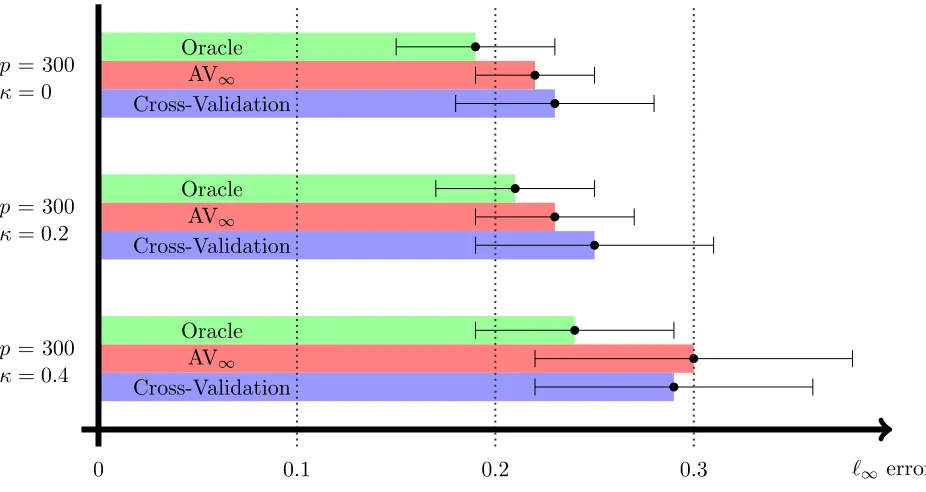
We simulate data from linear regression models as in equation (Model) with n = 200 observations and p ∈ {300,900} parameters. More specifically, we sample each row of the design matrix X ∈ _Rn×p _{from a} _p_{-dimensional normal distribution with mean 0 and}

covariance matrix (1−κ) I +κ1l, where I is the identity matrix, 1l : = (1, . . . ,1)>(1, . . . ,1) is the matrix of ones, and κ ∈ {0,0.2,0.4} is the magnitude of the mutual correlations. For the entries of the noiseε∈_Rn_{, we take the one-dimensional normal distribution with mean}

0 and variance 1. The entries of β∗ are first set to 0 except for 6 uniformly at random chosen entries that are each set to 1 or −1 with equal probability. The entire vector β∗ is then rescaled such that the signal-to-noise ratio kXβ∗k2

2/n is equal to 5. We finally

consider a grid of 100 tuning parameters Λ :={λmax/1.30, λmax/1.31, . . . , λmax/1.399}with

λmax : = 2kX>Yk∞/n. We run 100 experiments for each set of parameters and report

the corresponding means (thick, colored bars) and standard deviations (thin, black lines). All computations are conducted with the software R (R Core Team, 2013) and the glmnet package (Friedman et al., 2010). While we restrict the presentation to the parameter settings described, we found similar results over a wide range of settings.

We compare the sup-norm and variable selection performance of the following three procedures:

- Oracle: Lasso with the tuning parameter that minimizes the `∞ loss (this tuning

parameter is unknown in practice);

- AV∞: Lasso with AV∞ and C= 0.75;

- Cross-Validation: Lasso with 10-fold Cross-Validation.

(9)

p = 300 κ= 0.4

Oracle AV∞

Cross-Validation p = 300

κ= 0.2

Oracle AV∞

κ= 0

Oracle AV∞

Cross-Validation

`∞ error

0 0.1 0.2 0.3

Figure 1: Sup-norm error kβb_λ−β∗k∞ of the Lasso with three different calibration schemes

(10)

p = 900 κ= 0.4

Oracle AV∞

κ= 0.2

Oracle AV∞

κ= 0

Oracle AV∞

Cross-Validation

`∞ error

0 0.1 0.2 0.3

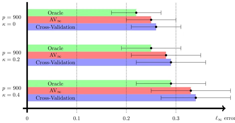
Figure 2: Sup-norm error kβb_λ−β∗k∞ of the Lasso with three different calibration schemes

(11)

p = 300 κ= 0.4

AV∞ false positives

Cross-Validation false positives

AV∞ false negatives

Cross-Validation false negatives p = 300

κ= 0.2

κ= 0

Cross-Validation false negatives

Variable selection error

0 20 40 60

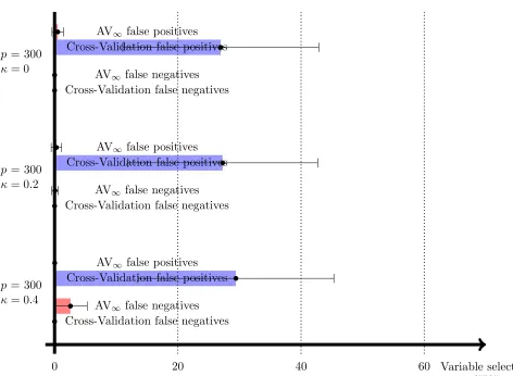
Figure 3: Number of false positives |{j : β_j∗ = 0,(βb_λ)_j 6= 0}| and false negatives |{j :

β_j∗ 6= 0,(βb_λ)_j = 0}| of the Lasso with AV_∞ and Cross-Validation as calibration

schemes for the tuning parameterλ. For AV∞, the safe threshold described after

(12)

p = 900 κ= 0.4

κ= 0.2

κ= 0

0 20 40 60

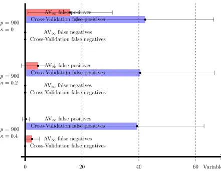
Figure 4: Number of false positives |{j : β_j∗ = 0,(βb_λ)_j 6= 0}| and false negatives |{j :

β_j∗ 6= 0,(βb_λ)_j = 0}| of the Lasso with AV_∞ and Cross-Validation as calibration

schemes for the tuning parameterλ. For AV∞, the safe threshold described after

(13)

Sup-norm error: In Figures 1 and 2, we compare the `∞ error of the four procedures.

We observe that AV∞ outperforms Cross-Validation for most settings under consideration.

We also mention that the same conclusions can be drawn if the normal distribution for the noise is replaced by other, possibly heavy-tailed distributions (for conciseness, we do not show the outputs).

Variable selection: In Figures 3 and 4, we compare the variable selection performance of AV∞ and Cross-Validation. More specifically, we compare the number of false positives

|{j : β_j∗ = 0,(βb_λ)_j 6= 0}| and the number of false negatives |{j : β_j∗ 6= 0,(βb_λ)_j = 0}|.

In contrast to Cross-Validation, AV∞ allows for a safe threshold of size 3Cλˆ (recall the

discussion after Theorem 3). Therefore, we report the results of Lasso with AV∞ and

an additional threshold of size 3Cλˆ applied to each component (that is, we consider the vector with entries (βb_λ)_j1l{|(βb_λ)_j| ≥3Cλˆ}), and we report the results of Lasso with

Cross-Validation (without threshold). We observe that, as compared to Cross-Cross-Validation, AV∞

with subsequent thresholding can lead to a considerably smaller number of false positives, while keeping the number of false negatives on a low level. Note that one could perform a similar thresholding of the Cross-Validation solution, but unlike for AV∞, there is no theory

to guide the choice of the threshold. This problem also applies to other standard calibration schemes.

Computational complexity: Cross-Validation with 10 folds requires the computation 10 Lasso paths, while AV∞ requires the computation of only one Lasso path - or even less.

AV∞ is therefore about 10 times more efficient than 10-fold Cross-Validation.

Let us conclude with remarks on the scope of the simulations. First, many meth-ods have been proposed for tuning the regularization parameter in the Lasso, includ-ing Cross-Validation, BIC and AIC-type criteria, Stability Selection (Meinshausen and Bühlmann, 2010), LinSelect (Baraud et al., 2014; Giraud et al., 2012), permutation ap-proaches (Sabourin et al., 2015), and many more. On top of that, there are many modifica-tions and extensions of the Lasso itself, including BoLasso (Bach, 2008), Square-Root/Scaled Lasso (Antoniadis, 2010; Belloni et al., 2011; Städler et al., 2010; Sun and Zhang, 2012), SCAD (Fan and Li, 2001), MCP (Zhang, 2010), and others. Detailed comparisons among the selection schemes and the methods can be found in the cited papers. We also refer to Leeb and Pötscher (2008) for theoretical insights about limitations of the methods.

In our simulations, we instead focus on the Lasso and, since we are not aware of guar-antees similar to ours for any selection scheme, we compare to the most popular and most extensively studied selection scheme, Cross-Validation. This comparison shows that, be-yond its theoretical properties and the easy and efficient implementation, AV∞ is also a

competitor in numerical experiments.

3.2 Riboflavin Production in B. subtilis

We now consider variable selection for a data set that describes the production of riboflavin (vitamin B2) in B. subtilis (Bacillus subtilis), see (B¨uhlmann et al., 2014). The data set

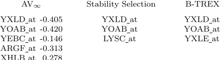
comprises the expressions of p = 4088 genes and the corresponding riboflavin production rates forn= 71 strains ofB. subtilis. We apply AV∞ and then impose the threshold 3Cλˆ.

(14)

AV∞ Stability Selection B-TREX

YXLD at -0.405 YXLD at YXLD at YOAB at -0.420 YOAB at YOAB at YEBC at -0.146 LYSC at YXLE at ARGF at -0.313

XHLB at 0.278

Table 1: Variable selection results for the riboflavin data set. The first column depicts the genes and the corresponding parameter values yielded by AV∞. The second and

third column depict the genes returned by approaches based on Stability Selection and TREX.

approaches based on Stability Selection (B¨uhlmann et al., 2014) and TREX (Lederer and M¨uller, 2015), which are given in the third and fourth column.

4. Conclusions

We have introduced a novel method for sup-norm calibration, known as AV∞, that is

equipped with finite sample guarantees for estimation in`∞-loss and for variable selection.

Moreover, we have shown that AV∞allows for simple and fast implementations. These

prop-erties make AV∞ a competitive algorithm, as standard methods such as Cross-Validation

are computationally more demanding and lack non-asymptotic guarantees.

In order to bring sharp focus to the issue, we have focused this paper exclusively on the calibration of the Lasso. However, we suspect that the methods and techniques developed here could be more generally applicable, for instance to problems with nonconvex penalties (e.g., SCAD, MCP). In particular, the paper (Loh and Wainwright, 2014) provides guar-antees for `∞-recovery using such nonconvex methods, which could be combined with our

results. Another interesting direction for future work is the use of our methods for more general decomposable penalty functions (Negahban et al., 2012), including the nuclear norm that is often used in matrix estimation.

We also stress that our goals are`∞-estimation and variable selection, which are feasible

only under strict conditions on the design matrix. Other objectives, including prediction and `2-estimation, can typically be achieved under less stringent conditions. However, the

corresponding oracle inequalities contain quantities (such as the sparsity level) that are typically unknown in practice. Adaptations of our method to objectives beyond the ones considered here thus need further investigation. We refer to (Ch´etelat et al., 2014) for ideas in this direction. However, there might be no approach that is uniformly optimal for all objectives, see also the papers (Yang, 2005; Zhao and Yu, 2006).

Finally, as pointed out by one of the reviewers, another field for further study is model misspecification. It would be interesting to see how robust the Lasso with the AV∞scheme

(15)

Acknowledgments

We thank Sara van de Geer and S´ebastien Loustau for the inspiring discussions. We also thank the reviewers for the careful reading of the manuscript and the insightful comments. This work was partially supported by NSF Grant DMS-1107000, and Air Force Office of Scientific Research AFOSR-FA9550-14-1-0016 to MJW.

Appendix A. Proof of Theorem 1

Define the event T_δ∗ : =

n_k X>εk∞

n ≤

λ∗_δ

4

o

and note that P[Tδ∗] ≥ 1−δ by our definition

of the oracle tuning parameter in (3). Thus, it suffices to show that the two bounds hold conditioned on the eventT_δ∗.

Bound on λˆ: To show that ˆλ ≤ λ∗_δ, we proceed by proof by contradiction. If ˆλ > λ∗_δ, then the definition of the AV∞method implies that there must exist two tuning parameters λ0, λ00≥λ∗_δ such that

kβb_λ0−βb_λ00k∞> C(λ0+λ00). (11)

However, sinceT_λ0 andT_λ00are both subsets ofT∗

δ , Assumption`∞(C) implies that we must

have the simultaneous inequalitieskβb_λ0−β∗k_∞≤Cλ0 andkβb_λ00−β∗k_∞≤Cλ00. Combined with the triangle inequality, we find that

kβb_λ0 −βb_λ00k∞≤ kβb_λ0 −β∗k∞+kβ∗−βb_λ00k∞ ≤ C(λ0+λ00).

SinceC≥C, this upper bound contradicts our earlier conclusion (11) and, therefore, yields the desired claim.

Bound on the sup-norm error: On the eventT_δ∗, we have ˆλ≤λ∗_δ, and so the AV∞

def-inition implies that

kβb_ˆ

λ−βbλ∗δk∞≤C

ˆ

λ+λ∗_δ ≤ 2Cλ∗_δ.

Combined with the triangle inequality, we find that

kβb_ˆ λ−β

∗_k

∞≤ kβb_ˆ

λ−βbλ∗δk∞+kβbλ

∗

δ−β ∗_k

∞≤2Cλ∗_δ+kβb_λ∗

δ −β ∗_k

∞.

Finally, underT_δ∗ and C≥C, Assumption`∞(C) implies thatkβb_λ∗

δ−β ∗_k

∞≤Cλ∗_δ ≤Cλ∗_δ,

and combining the pieces completes the proof.

Appendix B. Remaining Proofs for Section 2

(16)

B.1 Proof of Lemma 5

By the first-order stationarity conditions for an optimum, the Lasso solutionβb_λmust satisfy

the stationary condition 1_nX> Xβb_λ −Y

+λz_b = 0, where z_b ∈ _Rp _{belongs to the}

sub-differential of the `1-norm atβb_λ. Since Y =Xβ∗+ε, we find that

b

Σ βb_λ−β∗

=−λzb+

X>ε n .

Taking the `∞-norm of both sides and applying the triangle inequality yields

kbΣ βb_λ−β∗

k∞≤λkbzk∞+

X>ε n

_∞

≤λ+λ

4 = 5 4λ,

using the bound from event T_λ, and the fact that kz_bk∞ ≤ 1, by definition of the `1

-sub-differential. As noted previously, under the eventTλ, the error vector∆ =b βb_λ−β∗ belongs

to the coneC(S) in (6), so that theγ-RE condition can be applied so as to obtain the lower

boukΣ(b βb_λ−β∗)k∞≥γkβb_λ−β∗k∞. Combining the pieces concludes the proof.

Since ∆∈_C(S), we have

k∆k2₁ ≤9k∆Sk21 ≤9|S|k∆Sk22≤9|S|k∆k22≤9|S|k∆k1k∆k∞,

which implies k∆k₁ ≤ 9|S|k∆k∞. In view of Lemma 5, it thus suffices to prove the lower

bound

kΣ∆b k∞≥(1−ν)k∆k∞ for all ∆∈A: =B1(9|S|)∩B∞(1), (12)

where we set Bd(r) : ={β ∈Rp :kβkd≤r} ford∈[0,∞] and r≥0. We claim that

B1(9|S|)∩B∞(1)

| {z }

A

⊆2 cl conv

B0(9|S|)∩B∞(1)}

| {z }

B

, (13)

where cl conv denotes the closed convex hull. Taking this as given for the moment, let us use it to prove the desired claim. We have

max

∆∈A

k(Σb−I)∆k∞

k∆k∞

= max

∆∈A/2

k(Σb−I)∆k∞

k∆k∞

≤ max

∆∈B

k(Σb −I)∆k∞

k∆k∞

≤max

j∈[p]|Tmax|=9|S|

T⊂[p]\j X

k∈T

|bΣjk| ≤ ν

(14)

using the diagonal dominance (8). Combined with the triangle inequality, the lower bound (12) follows.

It remains to prove the inclusion (13). Since both A and B are closed and convex, it suffices to prove that φA(θ) ≤ φB(θ) for all θ ∈ Rp, where φA(θ) : = supz∈Ahz, θi and

(17)

subset indexing its top 9|S|values in absolute value. By construction, we are guaranteed to have the bound 9|S|kθTck_∞≤ kθ_Tk₁, and consequently

sup

z∈A

(hzT, θTi+hzTC, θ_TCi)φ_A(θ)≤sup

z∈A

(kzTk∞kθTk1+kzTCk₁kθ_TCk∞)

≤ kθTk1+ 9|S| kθTck_∞

≤ 2kθTk1.

On the other hand, for this same subset T, we have φB(θ) ≥ supz∈BhzT, θTi = 2kθTk1,

which completes the proof.

In order to prove Lemma 8, we use a somewhat simplified version of a recent result due to van de Geer (2014). So as to simplify notation, we first define the norms kak_j : = |aj|

and kak−j : =Pi6=j|ai|for any vector a. We then have:

Lemma 11 (van de Geer (2014), Lemma 2.1) Given any tuning parameter λ >0, it holds that

kβb_λ−β∗k_j ≤D_j

kX>εk∞

n +

p

log(p)kβb_λ−β∗k−j

2√nkηj_k

1

+λ 2

!

for all j= 1, . . . , p,

where for each j∈[p],

Dj : =

kηjk1

kXηj_k2 2/n+

p

log(p)/nkηj_k₋ j/2

.

This result provides a specific bound for each coordinate of Lasso. Lemma 8 can then readily be proven using this result together with Theorem 6.1 from B¨uhlmann and van de

Geer (2011).

Appendix C. Strong Correlations

In this paper, we assume that the correlations in design matrix are small, which is needed for precise `∞-estimation and variable selection. In the interest of completeness, however,

we add here two simulations where the correlations are large. Overall, we use the same settings as described in the main part of the paper, but we set κ = 0.9. The results are summarized in Figure 5 (note that the x-scale in the upper part of the figure is different from the scales of the corresponding plots in the main part of the paper). We find that AV∞ misses about half of the pertinent variables but has almost no false positives.

Cross-Validation, on the other hand, has less false negatives but selects many irrelevant variables. As expected, none of the methods, including the oracle, provide accurate`∞-estimation.

References

A. Antoniadis. Comments on: `1-penalization for mixture regression models. Test, 19(2):

(18)

p = 900 κ= 0.9

Oracle AV∞

κ= 0.9

Oracle AV∞

Cross-Validation

`∞ error

0 1 2 3

p = 900 κ= 0.9

κ= 0.9

0 6 20 40 60

Figure 5: Sup-norm and variable selection errors of the Lasso with three/two different cal-ibration schemes for the tuning parameter λ. Depicted are the results for two simulation settings that differ in the number of parameters p. The simulation settings and the calibration schemes are specified in the main part of the paper.

F. Bach. Bolasso: model consistent lasso estimation through the bootstrap. InProceedings of the 25th International Conference on Machine Learning, pages 33–40, 2008.

(19)

A. Belloni, V. Chernozhukov, and L. Wang. Square-root lasso: pivotal recovery of sparse signals via conic programming. Biometrika, 98(4):791–806, 2011.

P. Bickel, Y. Ritov, and A. Tsybakov. Simultaneous analysis of the Lasso and Dantzig selector. Ann. Statist., 37(4):1705–1732, 2009.

P. B¨uhlmann and S. van de Geer. Statistics for high-dimensional data: Methods, theory and applications. Springer Series in Statistics. Springer, 2011.

P. B¨uhlmann, M. Kalisch, and L. Meier. High-dimensional statistics with a view toward applications in biology. Annual Review of Statistics and Its Application, 1(1):255–278, 2014.

F. Bunea. Honest variable selection in linear and logistic regression models via`1and`1+`2

penalization. Electron. J. Stat., 2:1153–1194, 2008.

D. Ch´etelat, J. Lederer, and J. Salmon. Optimal two-step prediction in regression.

arXiv:1410.5014, 2014.

M. Chichignoud and J. Lederer. A robust, adaptive M-estimator for pointwise estimation in heteroscedastic regression. Bernoulli, 20(3):1560–1599, 2014.

A. Dalalyan, M. Hebiri, and J. Lederer. On the Prediction Performance of the Lasso.

Bernoulli, in press, 2014.

J. Fan and R. Li. Variable selection via nonconcave penalized likelihood and its oracle properties. J. Amer. Statist. Assoc., 96(456):1348–1360, 2001.

J. Friedman, T. Hastie, and R. Tibshirani. Regularization paths for generalized linear models via coordinate descent. Journal of Statistical Software, 33(1):1–22, 2010.

C. Giraud, S. Huet, and N. Verzelen. High-dimensional regression with unknown variance.

Statistical Science, 27(4):500–518, 2012.

M. Hebiri and J. Lederer. How correlations influence Lasso prediction.IEEE Trans. Inform. Theory, 59(3):1846–1854, 2013.

J. Lederer and C. M¨uller. Don’t fall for tuning parameters: Tuning-free variable selection in high dimensions with the trex. In Proceedings of the Twenty-Ninth AAAI Conference on Artificial Intelligence, 2015.

H. Leeb and B. P¨otscher. Sparse estimators and the oracle property, or the return of Hodges’ estimator. J. Econometrics, 142(1):201–211, 2008.

O. Lepski. A problem of adaptive estimation in Gaussian white noise. Teor. Veroyatnost. i Primenen., 35(3):459–470, 1990. ISSN 0040-361X.

O. Lepski, E. Mammen, and V. Spokoiny. Optimal spatial adaptation to inhomogeneous smoothness: an approach based on kernel estimates with variable bandwidth selectors.

(20)

P.-L. Loh and M. Wainwright. Support recovery without incoherence: A case for nonconvex regularization. arXiv:1412.5632, 2014.

K. Lounici. Sup-norm convergence rate and sign concentration property of Lasso and Dantzig estimators. Electron. J. Stat., 2:90–102, 2008.

N. Meinshausen and P. B¨uhlmann. Stability selection. J. R. Stat. Soc. Ser. B. Stat. Methodol., 72(4):417–473, 2010.

S. Negahban, P. Ravikumar, M. J. Wainwright, and B. Yu. A unified framework for high-dimensional analysis ofM-estimators with decomposable regularizers.Statistical Science, 27(4):538–557, December 2012.

R Core Team. R: A Language and Environment for Statistical Computing. R Foundation for Statistical Computing, Vienna, Austria, 2013. http://www.R-project.org/.

J. Sabourin, W. Valdar, and A. Nobel. A permutation approach for selecting the penalty parameter in penalized model selection. Biometrics, 71(4):1185–1194, 2015.

N. St¨adler, P. B¨uhlmann, and S. van de Geer. `1-penalization for mixture regression models.

Test, 19(2):209–256, 2010.

T. Sun and C.-H. Zhang. Scaled sparse linear regression. Biometrika, 99(4):879–898, 2012.

R. Tibshirani. Regression shrinkage and selection via the lasso. J. Roy. Statist. Soc. Ser. B, 58(1):267–288, 1996.

S. van de Geer. The deterministic Lasso. 2007 Proc. Amer. Math. Soc. [CD-ROM], see also www.stat.math.ethz.ch/˜geer/lasso.pdf, 2007.

S. van de Geer. Worst possible sub-directions in high-dimensional models. J. Multivariate Anal., in press, 2014.

S. van de Geer and P. B¨uhlmann. On the conditions used to prove oracle results for the Lasso. Electron. J. Stat., 3:1360–1392, 2009.

S. van de Geer and J. Lederer. The Lasso, correlated design, and improved oracle inequal-ities. IMS Collections, 9:303–316, 2013.

Y. Yang. Can the strengths of aic and bic be shared? A conflict between model indentifi-cation and regression estimation. Biometrika, 92(4):937–950, 2005.

F. Ye and C.-H. Zhang. Rate minimaxity of the lasso and dantzig selector for the lq loss in lr balls. J. Mach. Learn. Res., 11:3519–3540, 2010.

C.-H. Zhang. Nearly unbiased variable selection under minimax concave penalty. Ann. Statist., pages 894–942, 2010.