A Gibbs Sampler for Learning DAGs
Robert J. B. Goudie [email protected]
Medical Research Council Biostatistics Unit Cambridge CB2 0SR, UK
Sach Mukherjee [email protected]
German Centre for Neurodegenerative Diseases (DZNE) Bonn 53175, Germany
Editor:Peter Spirtes
Abstract
We propose a Gibbs sampler for structure learning in directed acyclic graph (DAG) mod-els. The standard Markov chain Monte Carlo algorithms used for learning DAGs are random-walk Metropolis-Hastings samplers. These samplers are guaranteed to converge asymptotically but often mix slowly when exploring the large graph spaces that arise in structure learning. In each step, the sampler we propose draws entire sets of parents for multiple nodes from the appropriate conditional distribution. This provides an efficient way to make large moves in graph space, permitting faster mixing whilst retaining asymp-totic guarantees of convergence. The conditional distribution is related to variable selection with candidate parents playing the role of covariates or inputs. We empirically examine the performance of the sampler using several simulated and real data examples. The proposed method gives robust results in diverse settings, outperforming several existing Bayesian and frequentist methods. In addition, our empirical results shed some light on the relative merits of Bayesian and constraint-based methods for structure learning.
Keywords: structure learning, DAGs, Bayesian networks, Gibbs sampling, Markov chain Monte Carlo, variable selection
1. Introduction
We consider structure learning for graphical models based on directed acyclic graphs (DAGs). The basic structure learning task can be stated simply: given data X on p variables, as-sumed to be generated from a graphical model based on an unknown DAG G, the goal is to make inferences concerning the edge set of G (the vertex set is treated as fixed and known). Structure learning appears in a variety of applications (for an overview see Korb and Nicholson, 2011) and is a key subtask in many analyses involving graphical models, including causal inference.
In a Bayesian framework, structure learning is based on the posterior distribution
P(G | X) (Koller and Friedman, 2009). The domain of the distribution is the space G
sample from the space of total orders (Friedman and Koller, 2003). Order-space sampling entails some restrictions on graph priors (Eaton and Murphy, 2007; Ellis and Wong, 2008), because the number of total orders with which a DAG is consistent is not constant. Order-space approaches have more recently led to exact methods based on dynamic programming (Koivisto and Sood, 2004; Parviainen and Koivisto, 2009; Tian and He, 2009; Tamada et al., 2011; Parviainen and Koivisto, 2013; Nikolova et al., 2013). These are currently feasible only in small domain settings (typically p < 20 but p < 30 is feasible on large cluster computers) and usually share the same restrictions on graph priors as order-space sam-plers. Frequentist constraint-based methods such as the PC-algorithm (Spirtes et al., 2000; Colombo and Maathuis, 2014) and the approach of Xie and Geng (2008) are an alterna-tive. These methods make firm decisions about the DAG structure via a series of tests of conditional independence.
In this paper we propose a Gibbs sampler for structure learning of DAGs that amelio-rates key deficiencies in existing samplers. Random-walk Metropolis-Hastings algorithms currently used for structure learning propose ‘small’ changes at each iteration, which can leave the algorithms unable to escape local modes. The Gibbs sampler proposed here con-siders the parents of a set of nodes as a single component (a so-called ‘block’), sampling an entire parent set for each node in the block in one step. These ‘large’ moves are sam-pled from the appropriate conditional posterior distribution. This enables the sampler to efficiently locate and explore areas of significant posterior mass. The method is based on the simple heuristic that the parents of a node are similar to the covariates or inputs in variable selection, with the node as the output variable, but accounts for acyclicity ex-actly so that the equilibrium distribution is indeed the correct posterior distribution over DAGs. The sampler does not impose restrictions on priors or graph space beyond those (maximum in-degree, modular prior) common to most samplers for structure learning (e.g. Friedman and Koller, 2003; Ellis and Wong, 2008; Grzegorczyk and Husmeier, 2008). The maximum in-degree restriction formally precludes large-sample consistency in the general case, but facilitates effective and robust inference by reducing the size of the model space (see Discussion).
2. Notation and Model
Let G denote a DAG with vertex set V(G) = {1, . . . , p}, and directed edge set E(G) ⊂ V(G)×V(G); often we will refer to vertex and edge sets simply as V and E respectively, leaving G implicit. The binary adjacency matrix corresponding to Gis denoted AG, with entries specified as AGuv = 1 ⇐⇒ (u, v) ∈ E(G) and diagonal entries equal to zero. For inference, G is treated as a latent graph in the space G of all possible DAGs with
p vertices. When a DAG is used to define a probabilistic graphical model (a Bayesian network), each vertex (or node; we use both terms interchangeably) is associated with a component of a p-dimensional random vector X = (X1. . . Xp)T. XZ denotes the random
variables (RVs) corresponding to variable indicesZ ⊆ {1, . . . , p}. We use bold type for the corresponding data; n samples are collected in the n×p matrix X, with Xu denoting the
column corresponding to variable uand XZ the submatrix corresponding to variable index
A graphG
1
2 3
4
AG=
0 1 1 0 0 0 1 0 0 0 0 0 0 0 1 0
paG
1 =∅
paG2 ={1}
paG3 ={1,2,4}
paG4 =∅
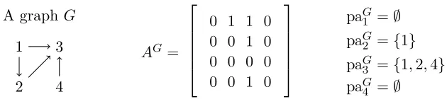
Figure 1: Illustration of notation. A graph G, with vertex set V = {1,2,3,4}, edge set
E={(1,2),(1,3),(2,3),(4,3)} and adjacency matrixAG as shown, can be spec-ified using parent sets as G = hpa1 = ∅,pa2 = {1},pa3 = {1,2,4},pa4 = ∅i or abbreviated toG=h∅,{1},{1,2,4},∅i(see text for description of notation). For the vertex subset Z ={2,4}, paGZ = ({1},∅) and paG−Z = (∅,{1,2,4}) and thus the graph can be specified as G = hpaZ = paGZ,pa−Z = paG−Zi. We abbreviate
this asG=hpaGZ,paG−Zi.
The proposed Gibbs sampler changes entire parent setsen masse, not just for one node but for a set of nodes, and so it will often be convenient and natural to specify a DAGGin terms of the parents of each node. Let paGv ={u : (u, v) ∈E(G)} denote the set of nodes that are parents of nodev inG. A tuple ofp parent sets hpa1 = paG1, . . . ,pap = paGpi fully specifies the edge set E, since u ∈paGv ⇐⇒ (u, v)∈ E(G). Thus, structure learning can be viewed as inference of parent sets pav. The parent set pav takes values in the power set
P(V \ {v}) of nodes excluding node v, subject to acyclicity. We will usually suppress the labels, and simply writehpaG1, . . . ,paGpi when specifying parent sets. Since paGv is a subset of the variable indices, we can use XpaG
v to denote the corresponding data submatrix.
We denote the tuple of parent sets of a set of nodes Z = {z1, . . . , zs} ⊆ V by paGZ =
(paG
z)z∈Z. This is a tuple of scomponents (for notational convenience we take these to be
ordered by increasing vertex index), each of which is the parent set for the corresponding node inG. We wish to make inferences about paZ, which takes values inP(V\ {z1})×. . .× P(V \ {zs}), subject to acyclicity. The tuple of parent sets for the complementZC=V \Z
is denoted paG−Z = (paGz)z∈ZC. Clearly, a tuple hpaGZ
1, . . . ,pa
G
Zsi of tuples of parent sets
specifies the parents of every node in a graph whenever {Z1, . . . , Zs} forms a partition of
V; the entire edge set can thus be specified by such a tuple. In particular, note that any graph G can be specified as hpaGZ,paG−Zi for any Z ⊂ V. Some of the notation we use is illustrated in Figure 1.
Our statistical formulation for Bayesian networks is standard. We briefly summarize the main points and refer the reader to the references below for details. Given a DAG G, the joint distribution ofX isp(X|G,{θv}) =Qv∈V p(Xv |XpaG
v, θv), i.e. the joint distribution
factors over nodes, and each node is conditioned on its parents in G, parameterized byθv.
For structural inference, interest focuses on the posterior distribution P(G | X). This is proportional to the product of the marginal likelihoodp(X|G) and a graph priorπ(G). Our sampler is compatible with essentially any specific model, but inherits computational costs associated with evaluation of the relevant quantities. In all examples we assume conjugate priors for θv, as well as local parameter independence and modularity; this leads to a
(Geiger and Heckerman, 1994) cases. Computations are simplified if the graph prior is modular (Friedman and Koller, 2003), meaning it factorises as π(G) =Q
v∈V πv(paGv); we
assume modular priors in all examples. Note that the prior is not specified over the space of orders and so is not subject to the restrictions this entails (Ellis and Wong, 2008; Eaton and Murphy, 2007). Under these assumptions, the posterior factorises across nodes as
P(G|X) =P(pa1= paG1, . . . ,pap= paGp |X)
∝ Y
v∈V
p(Xv |XpaG v)πv(pa
G v),
wherep(Xv |XpaG
v) is the marginal likelihood for nodevgiven the graphG=hpa G
1, . . . ,paGpi.
The distribution P(G|X) is the target distribution for our sampler.
3. A Gibbs Sampler for Structure Learning
In this section we provide a high-level description of the Gibbs sampler for structure learn-ing. We first recall the standard random-walk Metropolis-Hastings sampler (known as MC3)
and then describe a na¨ıve Gibbs sampler, which offers no gains over MC3, but prepares the ground for the introduction of ideas from the Gibbs sampling literature. Specifically we discuss a strategy known as blocking that can improve mixing in Gibbs samplers and show how to use blocking for structure learning of DAGs. Several points relating to computa-tion are central to developing a practical Gibbs sampler in this setting, but for clarity of exposition we defer discussion of computational aspects to Section 4.
3.1 MC3 Sampler
The standard sampler for structure learning of DAGs is MC3 (Madigan and York, 1995). This is a classical Metropolis-Hastings sampler with proposalG0drawn uniformly at random from the set neigh(G) of DAGs that differ from the current DAG G by the addition or removal of a single edge. The acceptance probability is min(1, r(G0, G)), where
r(G0, G) = min
(
1,P(G
0 |X)|neigh(G0)|−1 P(G|X)|neigh(G)|−1
)
.
Variants of MC3include single-edge direction reversal proposals (Giudici and Castelo, 2003). 3.2 A Na¨ıve (and Inefficient) Gibbs Sampler
Constructing a Gibbs sampler that is analogous to MC3 is straightforward. The posterior distribution on DAGs is a joint distribution over the off-diagonal entries in the adjacency matrix AG, i.e. over the p(p−1) binary RVs AGuv, u 6=v. At each iteration, MC3 can be thought of as proposing to toggle the value AGuv for some u 6=v, subject to the restriction that the resulting graph must be acyclic.
A simple Gibbs sampler works in a similar way. At each step, a move from graph Gto a new graph G0 is chosen by sampling from the conditional distribution of AGuv0 (for some
v; conversely, if (u, v) ∈/ E(G), define G−(u,v) to be identical to G, and G(u,v) to be the graph that differs from Gonly in including an edge from u tov. If G(u,v) is cyclic,G−(u,v)
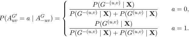
is sampled as the new graph G0 with probability 1. If G(u,v) is acyclic, the conditional distribution of AGuv0 is Bernoulli, i.e.
P(AGuv0 =a|AG−uv) =
P(G−(u,v)|X)
P(G−(u,v) |X) +P(G(u,v)|X) a= 0, P(G(u,v)|X)
P(G−(u,v) |X) +P(G(u,v)|X) a= 1.
The choice ofuandvcan either be made sequentially (systematically) or randomly (Roberts and Sahu, 1997); in this paper, random-scan Gibbs samplers are used throughout. We prove convergence of the Gibbs sampler to the target distribution in Appendix A.
3.3 Inefficiency in Gibbs Sampling
The mixing of Metropolis-Hastings samplers depends upon the proposal distribution, which for convenience is often chosen as a random-walk. In contrast, Gibbs samplers make moves according to conditional distributions that reflect local structure of the target distribution. Nonetheless, Gibbs sampling is not always efficient. In particular, correlation between the components being sampled can lead to inefficiency. To see this, consider a Gibbs sampler for a multivariate continuous distribution with highly correlated components. At each step, a single component is sampled according to its conditional distribution, but since it is strongly correlated with other component(s), the conditional is concentrated on only a small part of the support. This means the sampler is likely to make only small moves. Analogous issues arise with discrete distributions.
For graphical models based on DAGs, there may be strong dependence between the edge indicators AGuv, particularly for the collections of RVs corresponding to parent sets. For example, there may be RVs Xu and Xv that in combination score highly as parents
of node w, but not individually. Then, AGuw and AGvw will be correlated. In addition, the acyclicity restriction may induce strong dependence. For example, suppose two RVs
Xu and Xv are strongly correlated and both edges (u, v) and its reverse (v, u) have high
(a) w
y
x (b) w
y x
Figure 2: Illustrative scenario in which small local moves limit transitions between two regions of high probability. If both graphs (a) and (b) have high probability, the near-cyclic nature of the graphs makes transitions between (a) and (b) difficult.
3.4 A Gibbs Sampler with Blocking
We address the deficiencies of the na¨ıve Gibbs sampler by grouping a number of the compo-nents together and sampling from their joint conditional distribution. In Gibbs sampling, this is known asblocking. Sampling from such a joint conditional can ameliorate difficulties caused by correlations between components because the joint conditional naturally accounts for the correlation structure. In the multivariate normal case, Roberts and Sahu (1997) have shown that blocking improves convergence for random-scan Gibbs sampling.
In principle, any group of components can be taken as a block, but for the algorithm to be useful in practice, sampling from a block’s joint conditional distribution must be feasible, and ideally simple. The blocks that we consider correspond to groups (specifically tuples) of parent sets, so that the parent sets of several nodes are considered simultaneously. It is natural that each block is a tuple of parent sets because, as described in Section 2, we can specify a graphG using a tuplehpaG1, . . . ,paGpi of parent sets. It is therefore convenient to describe the sampler using this alternative graph specification, in whichG=hpaG1, . . . ,paGpi. We denote the set of q nodes whose parent sets will be sampled together as a block by
W ={w1, . . . , wq} ⊆V. Suppose the current graph is G= hpaGW,paG−Wi (recall that any
graph can be written in this way with respect to any partition of the node set). A move to a new graph G0=hpaGW0,paG−0Wi is formed by changing the parents of the nodes in W from paGW = (paGw1, . . . ,pawqG ) to paGW0 = (pawG01, . . . ,paGwq0) and setting paG−0W = paG−W (i.e. leaving the parents of nodes not inW unchanged). We sample the tuple paGW0 of parent sets jointly, conditional on the tuple paG−W of parent sets of nodes not inW (that remain unchanged). In terms of the adjacency matrix AG, each block consists of the indicators specifying the parents of the nodes in W, i.e.AGvw forv∈V, w∈W, v6=w.
To construct a Gibbs sampler using these blocks, we need to find the conditional pos-terior distribution on the tuple paW of parent sets, given that the remaining tuple pa−W of parent sets is set to paG−W. The conditional distribution depends on whether the graph
G0 formed using the proposed parent sets is acyclic. We therefore introducePaGW to denote the set of permissible tuples, i.e. tuples paGW0 of parent sets such that G0 = hpaGW0,paG−Wi
Algorithm 1 A Gibbs sampler for learning DAGs, with blocks
Initialise starting point G0 =hpaG0
1 , . . . ,paGp0i
for tin 1 to N do
Sampleq nodes uniformly at random from V, and call this set of nodes W
Sample paGW0 from P(paW = paGW0 |paGt−1
−W ,X)
SetGt←G=hpaG
0
W,pa Gt−1
−W i
end for
conditional probability is
P(paW = paGW0 |pa−W = paG−W,X) =
P(hpaG0
W,paG−Wi |X)
P(paG−W |X)
= P(G
0 |X)
P
paG00
W ∈PaGW P(pa G00
W ,paG−W |X)
. (1)
This is the conditional distribution needed to specify the blocked Gibbs sampler; Algo-rithm 1 outlines the procedure at a high level, with the setW of nodes chosen uniformly at random at each step. Asymptotic convergence follows from the argument in Appendix A (in fact the requirements on the graph prior will be weaker than in the na¨ıve case).
3.5 Tuning Parameters
To reduce the computational costs of structure learning it is common to set a maximum in-degree (e.g. Friedman and Koller, 2003; Grzegorczyk and Husmeier, 2008). We set a maximum in-degree κ = 3 in all empirical examples, except where stated otherwise (Sec-tion 5). This facilitates sampling from the condi(Sec-tional distribu(Sec-tion in Equa(Sec-tion 1 by re-ducing the computational cost of evaluating the normalising constant. We set the block size q = |W| = 3. While q can be chosen freely in principle, evaluating the conditional distribution in Equation 1 becomes unmanageable when q is large. Thus, both κ and q
act as tuning parameters (and are in addition to any hyper-parameters in the Bayesian formulation).
3.6 Structure Learning and Variable Selection
It is interesting to note that when q= 1 (and thusW =w for somew∈V) if no choice of parent set induces a cycle then PaGW =P(V \ {w}), the power set of the remaining nodes. In this case, the conditional distribution in Equation 1 can be viewed as the posterior distribution of a variable selection problem with response or output variable w, and the other variables as covariates or inputs. If the addition of particular nodes introduces a cycle, we have a constrained problem. In particular, suppose adding any of the nodes
4. Computational Aspects
Designing a computationally efficient sampler is not straightforward in this setting. To see why, note that to sample from the conditional in Equation 1 we need to be able to iden-tify the set PaGW of tuples of parent sets that is permissible (in the sense of maintaining acyclicity). The cardinality of this set is typically large, and the interdependence between the parent sets of each node inW makes decomposing the problem into subproblems non-trivial. A simple but na¨ıve approach would list all possible parent sets for each node inW
and check each such combination for cyclicity, but this approach is slow and cumbersome. We propose a partitioning scheme that leads to a two-stage sampler. The key idea is to choose the partition of PaGW so that, conditional on a component of the partition, the parents of each node are independent. This enables an efficient two-stage sampling method that we describe in Section 4.3. Acyclicity constraints are met by an efficient dynamic algorithm.
4.1 A Partition on Permissible Tuples of Parent Sets
We partition the setPaGW of permissible tuples of parent sets asPaGW ={PaG,H1
W , . . . , Pa G,Hη W }.
Each componentPaG,HhW is a set of permissible tuples of parent sets for nodes inW. It is con-venient to label the partition components using secondary (unrelated toG) DAGs Hh ∈ H,
whereHis the space of DAGs withq =|W|vertices;η is the cardinality ofH. We describe the relationship between eachPaG,HhW and DAGHhusing the following elements, illustrated
in Figure 3 and Table 1:
• The reduced graph G = hpaG
1, . . . ,paGpi, which is a function of the graph G, and is
identical to Gexcept that edges directed into nodes in W are removed.
paGw =
(
∅ w∈W,
paGw w /∈W
• The (reflexive) transitive closure, which is the directed graph TG on nodes V with edges ET, where (u, v) ∈ ET if and only if u = v or a (directed) path from u to v
exists in G (i.e. there exists a sequence of nodes z1, . . . , zs ∈V(G), with z1 =u and
zs=v, such that (z1, z2),(z2, z3), . . . ,(zs−1, zs)∈E(G)).
• The descendant nodes deGw = {v ∈ V : TGwv = 1} and the non-descendant nodes ndGw ={v∈V : TGwv= 0}ofw∈W in the reduced graphG. Note thatw∈deGw and
w /∈ndGw by definition.
• The nodes ndG=T
w∈Wnd G
w that are not descendants in the reduced graphGof any
node in W.
• The nodes deG,Hw =S x∈paH
w de G
x that are descendants in the reduced graph G of any
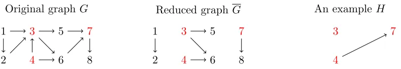
Original graphG 1 2 3 4 5 6 7 8
Reduced graphG
1 2 3 4 5 6 7 8
An example H
1 2 3 4 5 6 7 8
Figure 3: An illustrative example of the relevant graphs and sets, withW ={3,4,7}shown in red. The edges into W are removed from the original graph G, to form G. HereH is the set of all DAGs on the nodes {3,4,7} and thusη=|H|= 25. For
H as shown, ndG={1,2}.
deGw ndGw deG,Hw deG,H−w Q
G,H
w Condition (B)
w= 3 {3,5,6} {1,2,4,7,8} ∅ {3,4,5,6,7,8} {1,2} No restriction
w= 4 {4,6} {1,2,3,5,7,8} ∅ {3,4,5,6,7,8} {1,2} No restriction
w= 7 {7,8} {1,2,3,4,5,6} {4,6} {3,5,6,7,8} {1,2,4} paG70∩{4} 6=∅
Table 1: The relevant sets and requirements of conditions (A) and (B) for the illustrative graphGshown in Figure 3, withH as shown. Recall ndG={1,2}. Condition (B)
depends on RG,H7,4 = {4}, but it imposes no restriction when w ∈ {3,4} because paH3 = paH4 =∅. We find that PaG,HW contains all tuples of parent sets for which paG30 ⊆ {1,2}, paG40 ⊆ {1,2} and paG70 ={4} ∩Z whereZ ⊆ {1,2}.
• The nodes deG,H−w = S
x∈W\paH w de
G
x that are descendants in the reduced graph G of
any node x ∈ W \paHw, for a given node w ∈ W. Each node x ∈W \paHw is not a parent node ofw in the graph H=hpaHw1, . . . ,paHwqi.
Using this notation, we define PaG,Hw , for given G ∈ G, W ⊆ V, w ∈ W and H =
hpaH
w1, . . . ,pa
H
wqi ∈ H, as the set of parent sets paG
0
w that satisfy the following conditions.
(A) paGw0 ⊆QG,Hw =
ndG∪deG,Hw \deG,H−w
(B) paGw0∩RG,Hw,x =6 ∅for all nodes x∈paHw, with R G,H
w,x = deGx \de G,H
−w .
Note that (B) depends on deGx not deG,Hx . We define PaG,HW as the set of tuples formed by the Cartesian product of the sets PaG,Hw of parent sets for w ∈ W; in other words
paWG0 = (pawG10, . . . ,paGwq0)∈PaG,HW if and only if paGw10 ∈PaG,Hw1 , . . . ,paG 0
wq ∈Pa G,H wq .
Lemma 1 {PaG,H1
W , . . . , Pa G,Hη
W } is a partition of PaGW.
Condition (A) ensures all graphs G0 = hpaGW0,pa−GWi, with parents paGW0 ∈ PaG,HW , are acyclic. It requires that all parents of w ∈ W are either not descendants in the reduced graphGof any node inW, or a node whose ancestors in the reduced graphGare all parents in the graph H of nodew. In particular, no descendant of w is added as an ancestor of w. Condition (B) ensures each DAG G0 is a member of PaG,HW for only a single H∈ H for any givenG∈ G and thus that{PaG,H1
W , . . . , Pa G,Hη
W }is a partition of the set of permissible
tuples of parent sets. The condition checks that each edge in the graph H is ‘used’ i.e. that paGW0 = (paGw10, . . . ,paGwq0) ∈ PaG,HW would not be allowed under any H0 6=H, H0 ∈ H. Specifically, it ensures that each parent set paGw0 contains at least one descendant nodev∈V
of each parent paHw of node w in the graph H, and that v is not a descendant in G of any node x ∈ W that is not a parent in H of w ∈W. To see why this condition is required, consider a graphG0 in which all nodes inW have no parents. Then paGw0 =∅for all nodes
w ∈ W and so condition (A) holds for all H ∈ H. Thus if condition (B) is disregarded, paGW0 ∈PaG,HW for allH∈ H, implying that{PaG,H1
W , . . . , Pa G,Hη
W }is not a partition ofPaGW.
4.2 Fast Identification of Partition Components
Parent sets in each set PaG,Hw can be identified easily using simple set operations, and
consequently the partition componentsPaG,HW can be easily identified via Cartesian products of these sets. Let Paallw =P(V \ {w}) denote the set of all possible parent sets of node w, subject to maximum in-degree κ, and Paallw(v) = Paallw \ P(V \ {w, v}) denote the subset of Paallw containing only parent sets that contain node v ∈ V. Parent sets in PaG,Hw must
(A) not include any nodesnot inQG,Hw , and (B) include at least one node inRG,Hw,x for each
x∈paHw, and thus
PaG,Hw =
(
Pa(wB)\Paw(A) if paHw 6=∅
Paallw \Paw(A) if paHw =∅,
wherePa(wA)=Sv /∈QG,H w
Paall
w(v) and Pa
(B)
w =Tx∈paH w
S
r∈RG,Hw,x
Paall
w(r).
We fix q = |W| as a small constant for all p and set a maximum in-degree κ. This means permissible tuples of parents sets can be identified in O(pκ+1) time by storing the ‘lookup tables’ Paallw(v) as bit maps, assuming thatO(1) querying of the descendants and non-descendants is available.
This can be achieved using a dynamic algorithm that provides access to the transitive closure. Giudici and Castelo (2003) previously used a similar approach. For a graph with transitive closure TG with edges ET, the descendants and non-descendants of node u are
{v: (u, v) ∈ ET} and {v: (u, v) ∈/ ET} respectively. Thus, the descendants and non-descendants of a node can be identified inO(1) time when the transitive closure is known. The transitive closure for an arbitrary directed graph withp vertices can be determined in
transitive closure, and for incrementally updating it when an edge is added or removed from the graph. We choose to implement the algorithm introduced by King and Sagert (2002), which performs queries in O(1) time, and updates inO(p2) worst-case time (see reference for details of required assumptions). A trade-off exists between the performance of these two operations, but this bound for updates is thought to be the best possible whilst retaining
O(1) queries (Demetrescu and Italiano, 2005) and the algorithm is simple to implement. The algorithm maintains a p×p path count matrix CG whose elements CuvG are the number of distinct paths from nodeu to nodev in the graph Gforu6=v, and CuvG = 1 for
u =v. The transitive closure can be derived from the path count matrix by noting that TGuv = 1 if and only if CuvG > 0. Thus query operations are performed in O(1) by simply checking whether the relevant component of CG is positive. When an edge is added or removed CG is updated as follows. First consider adding an edge (u, v) to a graph G to form a new graphG0. The increase in the number of distinct paths between any two nodes
x and y is given by the (x, y) element of C∗Gu⊗CvG∗, where C∗Gu denotes the uth column of
CG,CvG∗ denotes thevth row and⊗denotes the outer product. Thus, the path count matrix is updated simply asCG0 =CG+C∗Gu⊗CvG∗. Similarly, when an edge (u, v) is removed from the graph the update isCG0 =CG−C∗Gu⊗CvG∗.
4.3 Two-stage Sampling Method
We draw a new graphG0 =hpaG0
W,paG−Wistarting from a graphGusing a two-stage method:
we sample first a componentPaG,HW 0 of the partition of permissible tuples of parent sets and then a tuple paGW0 of parent sets from the selected partition component.
In the first stage, PaG,HW 0 is drawn from the conditional distribution, given the tuple of parent sets of nodes not inW.
P(PaG,HW 0 |paG−W,X) =
P(PaG,HW 0,paG−W |X)
P(paG−W |X)
=
P
paG0 W∈Pa
G,H0 W
Q
w∈Wp(Xw |XpaG0
w )πw(pa G0
w )
P H00∈H
P
paG00 W ∈Pa
G,H00 W
Q
w∈W p(Xw |XpaG00
w )πw(pa G00
w )
=
Q w∈W
P
paG0 w∈Pa
G,H0
w p(Xw
|XpaG0
w )πw(pa G0
w )
P H00∈H
Q w∈W
P
paG00 w ∈Pa
G,H00
w p(Xw |XpaG
00
w )πw(pa G00
w )
The final equality follows by an interchange of sum and product that is proved in Lemma 2. This makes evaluation more efficient by allowing the sums to be evaluated separately for each node. Friedman and Koller (2003) used a similar interchange.
Lemma 2 The following identity holds for any H ∈ H, W ⊆V andG∈ G.
X
paW∈PaG,HW
Y
w∈W
p(Xw |Xpaw)πw(paw) = Y
w∈W X
paw∈Pa G,H w
p(Xw |Xpaw)πw(paw)
Algorithm 2 A Gibbs sampler for learning DAGs, with general blocks
Initialise starting point G0 =hpaG0
1 , . . . ,paGp0i
Compute initial path count matrix CG0 for tin 1 to N do
Sampleq nodes uniformly at random from V, and call this set of nodes W
LetG=Gt−1
FormGas defined in Section 4.1
Evaluate CG fromCG as described in Section 4.2
forw∈W do
Evaluate deGw ={v: CwvG ≥1}
Evaluate ndGw ={v : CwvG = 0} end for
forH ∈ Hdo forw∈W do
Evaluate PaG,Hw as described in Section 4.2
Let KwH =P
paG0 w∈Pa
G,H
w p(Xw |XpaG
0
w )πw(pa G0 w)
end for
LetKH =Q
w∈WKwH
end for
SamplePaG,HW 0 according toP(PaWG,H0 |paG−W,X) = KH
0 P
H00∈HKH
00 forw∈W do
Sample paG0
w according to P(paG
0
w |Pa G,H0
W ,paG−W,X)
end for
SetGt←G=hpaG
0
W,pa Gt−1
−W i
UpdateCGt end for
In the second stage, we sample new parents paG0
W from the selected partition component,
and form the new graph G0=hpaGW0,paG−Wi. The parents of each nodew∈W, conditional on H0, are independent, and so can be sampled separately from the following conditional distribution:
P(paGw0 |PaG,HW 0,paG−W,X) = p(Xw |XpaG
0
w )πw(pa G0 w) P
paG00 w ∈Pa
G,H0 w p(Xw
|XpaG00 w )πw(pa
G00
w )
.
This step is straightforward because this distribution is simply the posterior distribution of a constrained variable selection with response wand PaG,Hw 0 as the set of possible active
sets (i.e. selected covariates).
Algorithm 2 outlines the complete algorithm. The methods in Sections 4.2 enable fast identification of each partition component. Run-time is a function ofp, maximum in-degree
5. Results
In this section, we empirically assess the performance of the proposed sampler, comparing it with existing samplers as well as frequentist methods for structure learning of DAGs.
5.1 Evaluation Setup
We compare the Gibbs sampler with the MC3 sampler (Madigan and York, 1995) and the REV sampler (Grzegorczyk and Husmeier, 2008), a variant of MC3 that uses a more exten-sive edge reversal move. We also compare with two frequentist constraint-based methods: the PC-algorithm (Spirtes et al., 2000), and the Xie and Geng (2008) method, that is shown by its authors to outperform the PC-algorithm in some settings.
Tuning parameters for each method were set as follows. For the constraint-based meth-ods, the significance level was α = 0.05 by default, but we also show some results for
α = 0.00005,0.0001,0.0005,0.001,0.005,0.01,0.1. The Gibbs sampler we use is a random-scan sampler, with q = 3 (i.e. the parent sets of three nodes are sampled jointly at each iteration). To permit a fair comparison, for MC3 we use the same fast online transitive closure algorithm (Section 4.2), and pre-computation and caching of local marginal likeli-hoods used in the Gibbs sampler (REV uses a similar pre-computation and caching scheme). We constrain all of the samplers to maximum in-degree κ = 3 and set the graph prior as
π(G) ∝ 1. We use conjugate formulations throughout, specifically multinomial-Dirichlet (Heckerman et al., 1995) for discrete data and Normal with a g-prior (withg=n) (Geiger and Heckerman, 1994; Zellner, 1986) for continuous data.
We consider six examples: a small domain example, where comparison with the exact posterior (Tian and He, 2009) is possible; data simulated from the ALARM network and from randomly-generated networks of varying sparsity; data sets from social science and biology; and a pathological 4-node example designed to highlight a failure case for our method.
In practical use samplers can only be run for a finite number of iterations (depending on available time and computational resources). We set the maximum number of iterations as follows. In total, we drew 106 iterations of REV (retaining only every 10th iteration to re-duce storage requirements). Following Grzegorczyk and Husmeier (2008), 85% of proposals within REV were MC3 proposals (without MC3 proposals, the REV sampler is not irre-ducible). In our implementation, the computational costs of the Gibbs sampler are an order of magnitude lower than REV’s (accounting for MC3 moves), but we nevertheless treated
the computational costs as the same for the purposes of comparison and drew 106 iterations of the Gibbs sampler (again retaining every 10thiteration). The computational costs of our implementation of MC3 are roughly 1/10 of a Gibbs iteration, and so we performed 107 iterations of MC3 (retaining every 100th).
near a local rather than a global mode. We therefore also study convergence in detail via other metrics.
5.2 Evaluation Metrics
Each sampler gives an estimated posterior distribution over DAGs. From this we obtain a point estimate either as the maximum a posteriori (MAP) graph GMAP, or as a
thesholded graph Gτ formed by including all directed edges whose marginal posterior
edge probabilities are at least τ (note that Gτ need not be acyclic). When τ = 0.5 we
get themedian probability modelGmed (for normal linear models Barbieri and Berger, 2004, show that in some settings this is the optimal model for prediction). We also consider thresholding to match sparsity levels seen in frequentist point estimates, i.e. settingτ such that |E(Gτ)| = |E( ˆG)| for a point estimate ˆG. By GPCτ and GXieτ we denote thresholded
graphs whose sparsity is matched to the PC and Xie-Geng estimates respectively.
We use the structural Hamming distance (SHD) to quantify differences between DAGs. This is the minimum number of edge insertions and deletions needed to transform one graph into another. Comparisons are made using completed partially directed acyclic graphs (Chickering, 2002a). To show the behaviour of the samplers at shorter MCMC run lengths some metrics are shown against iteration t. These are based on the final 3/4 of samples drawn up to t(except for log marginal likelihoods), and so may incorporate some samples drawn before convergence.
We assess convergence and stability via the following metrics:
• Trace plotsof log marginal likelihood against iteration t.
• Between-run agreement betweenposterior edge probabilities. These are visualized as scatter plots. When edge probabilities agree between a pair of runs, all points in the plot will lie close to the y=x line. We show two variants: a hexagonally-binned version, to avoid over-plotting (Carr et al., 1987); and a panelled plot, in which each panel shows one pair of runs. We also consider the number of edges with estimated posterior probability greater than 0.9 in one run, and less than 0.1 in another run. Such‘major discrepancies’ represent serious Monte Carlo artefacts.
of each sampler as a collection of 5 pairs of runs and calculate PSRF separately for each edge using the final three quarters of the samples drawn up to that point.
• For the real data, we assess stability under resampling (“shaking the data”) by comparing estimates across bootstrap samples.
For experiments in which the true data-generating graph G∗ is known we use the fol-lowing metrics to assess accuracy:
• Structural Hamming distance(SHD) between G∗ and the estimated graphs.
• Receiver-operating characteristic (ROC) curves. These show agreement be-tween G∗ and an estimate Gτ by plotting true positive against false positive rates
parameterized by threshold τ. We consider also the area under the ROC curve
(AUROC), focusing in particular on the small false positive rate region of the curve that is often of interest in applications.
Finally, when the posterior edge probabilities can be computed exactly (Tian and He, 2009) (i.e. in small p settings) we also consider the maximum and average absolute error in posterior edge probability, calculated across the set of all possible edges.
We note that while SHD and ROC scores are useful in assessing performance, they are not convergence measures, as they do not assess accuracy of the posterior distribution per se (to see why, consider a degenerate sampler that samples only G∗, giving perfect scores on SHD and ROC, but an incorrect posterior distribution).
5.3 Small Domain Comparison to Exact Posterior
We applied the methods to the Zoo data set (Newman et al., 1998) that records p = 17 (discrete) characteristics of n= 101 animals. The maximum log marginal likelihood found by the Gibbs and REV samplers was consistent across runs, but less so for the MC3sampler,
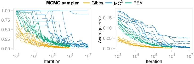
and the Gibbs sampler reached a plateau of high probability after the fewest iterations (Figure A13a). REV required about ten times as many iterations as Gibbs to achieve the same proportion of edges with PSRF < 1.1 while MC3 needed about 100 times as many (Figure A14a). The estimated edge probabilities given by the Gibbs sampler were stable between runs (Figure A15a). The results from the REV sampler were also stable, but MC3 less so, with major disparities between some runs. Figure 4 shows the error in posterior edge probabilities as a function of iterations. Convergence was quickest for the Gibbs sampler, followed by REV and then MC3. All runs of the Gibbs sampler reached a point at which the maximum absolute error was 0.05 (after 67,000 iterations on average). In contrast, only 5/10 runs of REV and 6/10 runs of MC3 reached the same level of accuracy in their complete run. Similarly, the Gibbs sampler achieved an average absolute error of less than 0.01 in the fewest iterations.
5.4 The ALARM Network
Figure 4: For the Zoo data set, maximum and average (across all possible 272 edges) error in posterior edge probabilities versus iteration number (on a log10scale). For each
MCMC algorithm, 10 independent runs, initialised at disparate initial values, are shown.
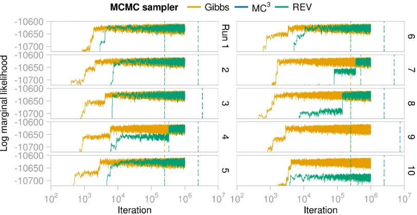
n = 100, 500, 1000, 2500, 5000. Figure 5 shows trace plots for the n = 1000 case as an illustrative example. The maximum log marginal likelihood found by the Gibbs sampler across runs was −10,608.20 ± 0.8 (mean ± standard deviation), whereas for REV it was
−10,627.2 ± 40.4 and for MC3 −11,176.9 ± 273.7. The highest scoring graph discovered by any of the 10 runs of the MC3 sampler had log marginal likelihood−10,856.6, far below
the Gibbs maximum, suggesting non-convergence in all 10 runs. REV appeared to reach convergence in all but two runs (runs 9 and 10). The Gibbs sampler consistently (and rapidly) reached a high scoring plateau and appeared to have converged in all 10 runs. PSRF results were in line with these findings (Figure A14b); more than 10 times as many iterations of REV were needed to give the same proportion of edges with PSRF <1.1 as the Gibbs sampler.
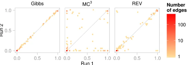
Figure 6 compares pairs of runs for n = 1000; this pair of runs is typical of all 10 runs (except for runs 9 and 10 of REV which disagree considerably; all runs shown in Figure A15b). There were no major between-run discrepancies (as defined in Section 5.2) for the Gibbs sampler at any sample size. The mean number of major discrepancies (across pairs of runs) increased from 0 (n= 100) to 8 and 91 for MC3 and REV respectively (when
n= 5000).
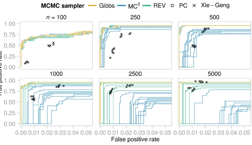
Figure 7 shows ROC curves for false positive rates <0.05. The Gibbs sampler performs better and with less variability than the other methods. Sample size is influential. For small
nthe Bayesian methods outperform the constraint-based methods. However, counter to the increase in statistical information, REV and MC3 perform less well with larger n: e.g. at
n= 100 for a false positive rate (FPR) of 0, the Gibbs sampler found 21.9±1.9 (mean±
standard deviation) true edges; REV 20.1±1.4; and MC3 21.7±2.1. But atn= 5000, for the same FPR, Gibbs found 43.0±0.0 true edges; REV 13.2±21.3; and MC3 did not find any true edges (the true graph has 46 edges). The constraint-based methods performed well for large sample sizes, as anticipated by the asymptotic consistency of the PC-algorithm (Kalisch and B¨uhlmann, 2007). The Xie-Geng method performed particularly well for
Figure 5: Log marginal likelihood of the graphs visited by the three MCMC samplers in 10 independent runs, initialised at disparate initial conditions, on the ALARM data, with data sample size n= 1000. Iteration number is displayed on a log10
scale. The dashed lines indicate where the burn-in phase ended. In all cases the log marginal likelihood of the graphs reached by the MC3 sampler are below the displayed range.
Figure 6: Convergence diagnostic plots for each MCMC sampler for the ALARM data, with
Figure 7: ALARM data, receiver operating characteristic (ROC) curves for each of 10 in-dependent MCMC runs for each MCMC sampler, and point estimates for the constraint-based methods. Note that the horizontal axis shows only false posi-tives rates < 0.05, corresponding to the case in which interest focuses on high-ranked edges (the complete curves are shown in Figures A16). Point estimates from Xie-Geng’s constraint-based method and the PC-algorithm are also shown for all 8 significance levels considered.
best after all run lengths and sample sizes considered. These results are supported by SHDs between point estimates and the true graph (Table A2).
5.5 Networks of Varying Sparseness
Sparsity can be used to statistical and computational advantage but in practice it may be hard to know what level of sparsity is reasonable for a given application. We therefore sought to investigate the effect of varying network sparsity, including scenarios where the data-generating graph can violate the in-degree constraint we impose. We simulated data following a procedure described in Kalisch and B¨uhlmann (2007) that we outline below. We first generated a DAG G via its adjacency matrix AG, by drawing entries as AGuv ∼
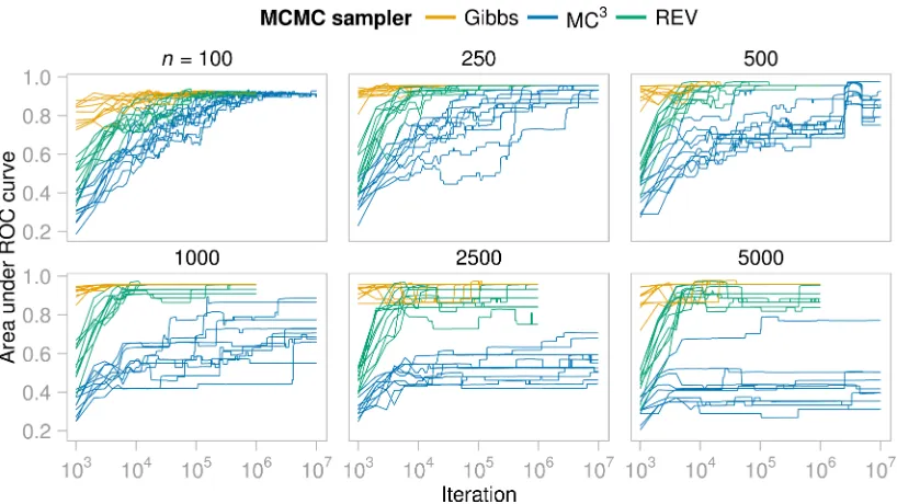
Figure 8: ALARM data, area under the receiver operating characteristic curve (AUROC) against iteration number (log10 scale) for each of the 10 independent runs for
each MCMC algorithm. Each panel shows results for a particular sample size
n= 100, . . . ,5000.
Figure 9 shows boxplots over SHDs. We see that accuracy decreases with increasing density, echoing results in Kalisch and B¨uhlmann (2007) for the PC algorithm. As through-out, all the samplers had an in-degree constraint (maximum in-degree κ = 3), while the frequentist methods did not. Nevertheless, the performance of the Bayesian methods did not appear to deteriorate any more rapidly than the frequentist methods. At all ρ’s, the median probability graph Gmed outperformed the frequentist methods which in turn out-performed the MAP graph. In this context, we draw attention to a difference between the median probability and MAP graphs: the former, although obtained by averaging over DAGs satisfying the in-degree constraint, may itself have in-degree greater than κ, while the latter is necessarily subject to the constraint.
5.6 Survey Data
Figure 9: Synthetic data, accuracy of estimation for networks with different levels of spar-sity. The panels correspond to simulations in which the expected number of neighbours for each node in the data-generating graph is respectively 2, 3, 4, 5, and 6. Accuracy is quantified by structural Hamming distance (SHD) between estimates and data generating graphs (smaller SHDs correspond to more accurate estimates). Box plots are over the 10 independent networks/data sets simulated for each sparsity level. For MCMC methods, results from the MAP graphGMAP
and median probability modelGmed are shown.
missing, to any of the 24 questions. The resulting sample size was n= 4,197. The median probability graphGmed estimated by the Gibbs sampler is shown in Figure A17a.
Figure 10 shows between-run agreement. The Gibbs runs showed better agreement than the REV runs and the MC3 runs disagreed considerably (these pairs of runs were typical; all runs shown in Figure A18a). Indeed there were no major between-run discrepancies (in the sense of Section 5.2) for the Gibbs sampler, whereas there were on average 2.4 major discrepancies for REV and 10.9 for MC3. The Gibbs sampler also had the highest proportion of edges with PSRF <1.1 (Figure A14c).
The maximum log marginal likelihoods found by each of the three samplers differed considerably as did the number of iterations needed to reach a plateau (Figure A13b). The Gibbs sampler typically reached a plateau after around 500 samples (although in one run 103 samples were needed). REV took longer to reach a (usually lower) plateau. MC3 appeared to become stuck in a region with even lower log marginal likelihood.
Figure 10: Convergence diagnostic plots for each MCMC sampler for the survey data. The posterior edge probabilities given by two independent MCMC runs are plotted against each other, binned into hexagonal areas to avoid over-plotting. When the two runs give the same estimates of the posterior edge probabilities all of the points appear on the line y = x; strongly off-diagonal points indicate extreme discrepancies between the runs. This pair of runs was typical of all pairs.
for the Bayesian methods (i.e. thresholding to give the same number of edges as PC), the mean SHD between results from pairs of bootstrap data sets was 21.7 (Gibbs), 22.3 (REV), 33.4 (MC3) and 30.8 (PC-algorithm). Results forGMAPandGXieτ are shown in Figure A19a.
5.7 Large-sample, Single-cell Molecular Data
We used single-cell molecular data from Bendall et al. (2011) with p = 34 continuous variables (see Appendix D) andn= 21,691. The median probability graphGmed estimated
by the Gibbs sampler is shown in Figure A17b.
Figure 11: Convergence diagnostic plots for each MCMC sampler for the single-cell molec-ular data. The posterior edge probabilities given by two independent MCMC runs are plotted against each other, binned into hexagonal areas to avoid over-plotting. When the two runs give the same estimates of the posterior edge probabilities all of the points appear on the line y = x; strongly off-diagonal points indicate extreme discrepancies between the runs. This pair of runs was typical of all pairs of runs.
network with a high density (recall that under GPCτ all methods choose the same number of edges as PC).
5.8 A Pathological 4-node Example
Our final example demonstrates the potential sensitivity of the Gibbs sampler to choice of
q=|W|(the number of nodes whose parent sets are sampled together in a single iteration). The example was constructed to highlight a situation in which the sampler can become stuck in a local mode unlessqis large enough, potentially leading to extremely slow convergence. We used as data 105 simulated samples from a 4-node network in which the parents of
node 2 were nodes 1 and 4; the parents of node 3 were nodes 1 and 2; and nodes 1 and 4 had no parents. Each node was Bernoulli distributed. The probability of success was 0.6 for nodes 1 and 4, while nodes 2 and 3 were noisy XORs with probability of success 0.9 when either parent (but not both) was ‘true’ and 0.1 otherwise.
For the purposes of demonstration, we set q = 2. As shown in Figure 12, after 106 iterations the maximum error in edge probability for the Gibbs sampler was 0.016±0.015 (mean ± standard deviation across 10 runs). Given that there are only 543 DAGs with
Figure 12: For the pathological 4-node example, maximum and average (across all possible 12 edges) error in posterior edge probabilities by iteration number (on a log10
scale). For each MCMC algorithm, 10 independent runs, initialised at disparate initial values, are shown.
setting q= 3 improved convergence (maximum error 0.0011 ±0.0009 after 106 iterations), but in real-world examples it is difficult to rule out the possibility that analogous issues may arise.
6. Discussion
We introduced a Gibbs sampler for structure learning of DAGs that can converge more easily than existing samplers due to its ability to efficiently make large moves in DAG space. We showed that it provides often substantial gains in accuracy and stability in comparison with existing (Bayesian and frequentist) methods in a range of settings.
The formulation of the sampler develops and exploits the connection between variable selection and structure learning. This connection has been widely studied for undirected graphs (e.g. Meinshausen and B¨uhlmann, 2006), but for DAGs is complicated by the acyclic-ity requirement. Our approach accounts for acyclicacyclic-ity but further work in this area may ease the adaptation of results and methods from Bayesian variable selection to the case of DAGs. In the proposed sampler, existing variable selection methods could be of direct utility in sampling from the conditional distribution P(paW |paG−W,X). When this sam-pling step is difficult, a Metropolis-within-Gibbs approach (i.e. substituting a Metropolis step in place of the Gibbs step) could be considered. With q = |W| = 1, the conditional
P(paW |paG−W,X) is identical to the posterior of the corresponding variable selection prob-lem. Then, a Metropolis-within-Gibbs move could directly exploit existing variable selection methods.
true number of parents of a node exceeds the restriction, important candidate parents may still have high edge scores (and appear in a summary graph). For example, suppose the true in-degree of a node is 4, but at most 3 incoming edges are permitted. In this case, although no model including all 4 parents can be considered, provided the signal can be detected considering only 3 nodes at a time, the posterior probability of all 4 edges may nonetheless be high.
In our empirical examples the REV sampler of Grzegorczyk and Husmeier (2008) showed impressive gains over MC3. The Gibbs sampler generally seemed to outperform both. The use of conditional distributions in REV is a point of similarity with the Gibbs sampler proposed here. The performance gains of Gibbs could be explained by two key differences from REV. First, REV does not use the natural conditional distribution and requires an accept-reject step. Second, REV must include at least some MC3 proposals (otherwise the sampler is not irreducible), and these steps are not tailored to the shape of the posterior distribution (Grzegorczyk and Husmeier, 2008, make REV proposals with probability 1/15 and so most steps are based on MC3 proposals).
If there is strong correlation between the parent sets of more than q = |W| nodes, the Gibbs sampler may not mix well. In this situation, constraint-based methods may be useful. Alternatively,qcould be chosen at each step according to some distribution, so that a mixture of different block sizes is used. This would in particular allow larger blocks to be used without increasing the computational demands of the algorithm excessively. In this paper we fixedq= 3, and found this simple choice gave a well-behaved and effective sampler. But there is a trade-off: increasingqincreases the time taken to evaluateP(paW |paG−W,X), but also increases move size, with the potential to improve convergence.
Practical use of the Gibbs sampler in the form described here requires exact sampling from the conditionalP(paW |paG−W,X) and there are situations related to this requirement in which other methods may be more suitable. First, when an appropriate maximum in-degree cannot be set, MC3 or a variant could be more appropriate (although convergence could be very slow). Alternatively, search procedures such as GES (Chickering, 2002b) or HCMC (Castelo and Koˇcka, 2003) could be used. Second, exact sampling from the condi-tional distribution is challenging in settings with thousands of nodes. In this case, efficient constraint-based methods (such as the PC-algorithm) may be a better choice, particularly in the large sample setting. As noted by a referee, an interesting area for future research would be combining the Gibbs sampler with some aspects of other methods—such as PC—that are relatively well suited to the truly high-dimensional setting.
Acknowledgments
supported by the Economic and Social Research Council (ESRC) and Engineering and Physical Sciences Research Council (EPSRC).
Appendix A. Convergence Conditions for Gibbs Samplers
Convergence of a Gibbs sampler for DAGs does not follow from the usual justification of Gibbs sampling that relies on the Hammersley-Clifford theorem (Besag, 1974). The theorem gives a positivity condition that is sufficient to prove that the univariate conditional distributions used by the Gibbs sampler uniquely define the joint distribution. The required condition is that the support of the joint distribution is given by the Cartesian product of the supports of the marginal distributions. An example of when this condition does not hold is the joint densityp(x, y) for a pair of random variables X and Y with support only on [0,1]×[0,1] and [2,3]×[2,3]. Clearlyp(x) andp(y) are both positive on [0,1] and [2,3] but neither [0,1]×[2,3] or [2,3]×[0,1] are in the support of the joint distribution (Hobert et al., 1997).
In the DAG setting, the acyclicity requirement means that this positivity condition is not satisfied. Consider a DAG consisting of two correlated random variables X1 and X2. The correlation means that both the graph with a single edge (1,2) and the graph with a single edge (2,1) have positive posterior probability. Thus P(AG12 = 1 | X) > 0 and
P(AG21= 1|X)>0 in the posterior marginal distributions. However, in the joint posterior distribution P(AG12 = 1, AG21 = 1| X) = 0 because the corresponding graph (the complete graph) is cyclic. The complete graph is thus not in the support of the joint distribution but is in the Cartesian product of the supports of the marginal distributions.
An alternative sufficient condition for uniqueness of the joint distribution and conver-gence of the Gibbs sampler when positivity is not satisfied is given by Besag (1994), which was extended for continuous settings by Hobert et al. (1997). In the present context, the condition requires that for every pairG0, G00∈ G of DAGs with pnodes there exists a finite sequence G1, . . . , GN, with G1 = G0, GN = G00 and N ∈ N, and such that Gt and Gt−1
differ in only a single component (in this context, a single edge), and that the joint poste-rior distribution P(Gt|X)>0 for all t= 0, . . . N. When the graph prior π(G)>0 for all
G∈ G, this condition is clearly satisfied: as an example, one such finite sequence removes every edge ofG0, one at a time, and then adds every edge ofG00, one at a time. Each graph in the sequence is clearly acyclic, since the sequence is composed of subgraphs of the acyclic
G0 and G00, and so has positive probability in the joint distribution when the graph prior is positive everywhere in G. A similar proof follows if the graph prior has support on all subgraphs of graphs with support in the graph prior, as is true for most widely used priors.
Appendix B. Proof of Lemma 1
Lemma 1 {PaG,H1
W , . . . Pa G,Hη
W } is a partition of PaGW.
Proof. We show: (i) S
h=1,...ηPa G,Hh
W ⊆ PaGW; (ii) S
h=1,...ηPa G,Hh
W ⊇ PaGW; and (iii)
PaG,Hh1
W ∩Pa G,Hh2
(i) We prove the relationship by showing that PaG,Hh W ⊆Pa
G
W for each h = 1, . . . , η. By
the definition ofPaGW in Section 3.4 we need to show thatG0 =hpaGW0,paG−Wiis acyclic for all tuples paG0
W ∈Pa G,Hh
W of parent sets, for all h= 1, . . . , η.
We proceed by contradiction. Suppose some graph G0 = hpaGW0,paG−Wi with paGW0 ∈ PaG,HhW is cyclic. First note that G is acyclic because Gis a subgraph of the acyclic
G. Since the graphG0 differs from the acyclic graph G only in the parents of nodes in W, each cycle in G0 must include at least one node in W. Denote by x1 x2
the existence of a path (that obeys the edge directions) in the graph G0 from node
x1 ∈W to node x2 ∈ W that does not include any nodes in W (except x1 and x2). Let w1, . . . , wr ∈ W be the (minimal) complete set of nodes in W included in some
cycle inG0. Without loss of generality suppose thatw1 w2 . . . wr inG0. Note
that sincew1, . . . , wr is the complete set of nodes inW in the cycle, no node between
wi and wi+1 in the path can be in W,i∈ {1, . . . , r−1}.
We now show that forx1, x2 ∈W,x1 x2 only if an edge (x1, x2) links nodex1 to x2 in the graph Hh. Since x1 x2, there must exist a node v ∈V that is a parent
of x2 in G0 such that v is a descendant in G0 of x1. Note that if the edge (x1, x2) is in the graph G0 then v = x1. Since v is a parent of nodex2 in the graph G0 and x2 ∈W, thenv∈ndG∪deG,Hhx2
\deG,Hh−x2 by condition (A). Also sincex1 x2 does
not include any nodes inW,v is also a descendant inGofx1 becauseG0 andGdiffer
only in which nodes are parents of nodes inW. We proceed by contradiction. Suppose no edge (x1, x2) exists in Hh. Then v is a descendant of x1 in the graph G, but x1
is not a parent of x2 in the graph Hh. So v ∈ deG,H−x2h, which by condition (A) is a
contradiction. Thusx1 x2 only if (x1, x2) is present in Hh, forx1, x2 ∈W.
Now, recall thatw1 w2 . . . wr. Since a cycle is formed we must in addition
have a path in G0 from node wr to node w1. Since w1, . . . , wr is the complete set of
nodes in W involved in the cycle, no node on the path from wr tow1 can be in W.
Thuswr w1. However, this implies that the edges (w1, w2),(w2, w3), . . . ,(wr−1, wr),
(wr, w1) are all in Hh, which implies Hh is cyclic. But Hh is acyclic by assumption,
and so we have a contradiction.
(ii) Suppose we start from a graph G = hpaGW,paG−Wi. We want to show that for each
DAGG0 =hpaGW0,paG−Wi there is someH0 ∈ Hsuch that paGW0 ∈PaG,HW 0. We will show that paGW0 ∈PaG,HW 0, where H0 =hpaH1 0, . . . ,paHq0i ∈ H is a DAG on nodes in W and pawH0 = {x ∈ W : there exists somev ∈ pawG0 such thatv ∈ deGx}. As usual, paGw0 is the parent set in the graphG0 of the nodew; and deGx is the descendants in G of the nodex. Note thatH0 is a subgraph (on the nodes inW) of the transitive closure TG0. By definition, G0 is a DAG, so TG0 is also a DAG, and thusH0 is a DAG.
For (A) we need paGw0 ⊆ ndG∪deG,Hw 0
\deG,H−w 0. Let v ∈paG
0
w meaning that v is a
parent of the nodew in the graphG0. First we show that v /∈deG,H−w 0, and then show
thatv∈ndG∪deG,Hw 0.
To show that v /∈ deG,H−w 0, note that if v ∈ deG,H−w0 then v must be a descendant in G
of some node y ∈ W that is not in paHw0. However, every such y is in paHw0 by the definition of paHw0, thusv /∈deG,H−w 0.
To show that v ∈ ndG∪deG,Hw 0, we suppose v /∈ ndG and show this implies that
v ∈ deG,Hw 0. This follows because if v /∈ ndG then it must be the descendant in G
of some node y ∈ W. Then y ∈ paHw0 by definition of H0. Therefore v ∈ deG,Hw 0, as required.
For (B), we need paGw0∩deGx \deG,H−w 0
6
=∅ for all x∈ pawH0. Consider x∈ paHw0. By the definition of paHw0, this means that there exists some node v ∈ paGw0 such that
v ∈ deGx. Additionally, any y ∈ W for which v ∈ deGy is such that y ∈ paHw0, by definition of paHw0. Thus v is not a descendant in G of any node in W that is not in paHw0. Thenv∈paGw0∩deGx \deG,H−w 0, and thus the condition is satisfied.
(iii) Since Hh1 6= Hh2, at least one node has different parents in Hh1 and Hh2. Suppose
that the nodew∈W is such a node, and thatx∈W is a parent ofw inHh1 but not
inHh2. Consider a parent set pa
G1
w ∈Pa G,Hh1
w . We will prove that paGw1 ∈/ Pa G,Hh2
w ,
and the result follows.
By condition (B), there must exist some v ∈ deGx \deG,Hh1
−w such that v ∈ paGw1. We
will show that v /∈ paG2
w for every parent set paGw2 ∈ Pa G,Hh2
w . This follows because
v ∈ deGx and so is a descendant inG of x, which is not a parent of w in Hh2. Thus
v∈deHh2
−w, and so v /∈
ndG∪deG,Hh2
w
\deG,Hh2
−w . Therefore v cannot be a parent of
winG2.
Appendix C. Proof of Lemma 2
Lemma 2 The following identity holds for any H∈ H, W ⊆V and G∈ G.
X
paW∈PaG,HW
Y
w∈W
p(Xw |Xpaw)πw(paw) = Y
w∈W X
paw∈Pa G,H w
p(Xw |Xpaw)πw(paw)
Proof. Define λ(wi) =p(Xw |Xpa(i)
w )πw(pa
(i)
w ), i∈ {1, . . .P}, where P is the cardinality of
PaG,HW , and where pa(wi) is the parent set of node w for the ith member of PaG,HW i.e. we
have that PaG,HW =
n
(pa(1)w1, . . . ,pa (1)
wq), . . . ,(pa(wP1), . . . ,pa (P)
wq) o
n
pa(1)w , . . . ,pa(wPw) o
, and thus Pw is the number of tuples of parent sets in PaG,Hw . Recall
thatPaG,HW is the Cartesian product of the sets PaG,Hw of parent sets forw∈W, thus
Y
w∈W
X
pa(wi)∈PaG,Hw
λ(wi)= Y
w∈W
λ(1)w +· · ·+λ(Pw) w
= X
i1∈{1,...,P1}, ..., iq∈{1,...,Pq}
λ(i1)
w1 . . . λ (iq)
wq
= X
(paw(i1),...,pawq(i))∈PaG,HW
λ(wi)1. . . λ(wqi)
= X
(paw(i1),...,pawq(i))∈PaG,HW Y
w∈W
λ(wi) .
Appendix D. Details of Data Analysed
We included in our analysis the following variables from the survey data (Centers for Dis-ease Control and Prevention, 2008): SEX, AGE G, RACEGR2, MARITAL, CHLDCNT, INCOMG, USEEQUIP, HCVU65,MEDCOST, SMOKER3, ASTHMST, RFDRHV3, RFBING4,QLREST2, RFSEAT3,
Appendix E. Additional Table
Method n= 100 250 500 1000 2500 5000
Gibbs 69.2±6.5 32.0±3.7 25.8±2.8 22.1±3.2 14.5±3.3 8.7±2.4 23.8±0.4 8.3±0.5 8.9±0.3 15.1±0.6 6.0±0.0 10.1±0.3 MC3 67.4±4.9 35.8±6.6 44.7±7.8 47.8±13.3 63.7±11.2 78.5±16.5 23.9±0.9 12.5±3.1 27.3±8.8 43.8±14.2 65.4±11.6 82.3±17.0 REV 68.2±5.5 34.7±5.8 27.4±4.6 28.1±4.0 24.4±9.5 20.4±6.7 25.9±2.1 8.3±1.1 4.0±0.0 11.5±2.0 11.6±9.9 13.5±8.0
PC 48.0 39.0 38.0 28.0 22.0 14.0
Xie-Geng 54.0 40.0 34.0 43.0 32.0 17.0
Appendix F. Additional Figures
Figure A13: Log marginal likelihood of the graphs visited by the three MCMC samplers in 10 independent runs, initialised at disparate initial conditions. In (A) Zoo data; (B) survey data; (C) single-cell molecular data. Iteration number is displayed on a log10 scale. The dashed lines indicate where the burn-in phase
References
M. M. Barbieri and J. O. Berger. Optimal predictive model selection. Annals of Statistics, 32(3):870–897, 2004.
I. A. Beinlich, H. J. Suermondt, R. M. Chavez, and G. F. Cooper. The ALARM monitoring system: A case study with two probabilistic inference techniques for belief networks. In Second European Conference on Artificial Intelligence in Medicine, pages 247–256. Springer-Verlag, Berlin, 1989.
S. C. Bendall, E. F. Simonds, P. Qiu, E. D. Amir, P. O. Krutzik, R. Finck, R. V. Bruggner, R. Melamed, A. Trejo, O. I. Ornatsky, R. S. Balderas, S. K. Plevritis, K. Sachs, D. Pe’er, S. D. Tanner, and G. P. Nolan. Single-cell mass cytometry of differential immune and drug responses across a human hematopoietic continuum. Science, 332(6030):687–696, 2011.
J. E. Besag. Spatial interaction and the statistical analysis of lattice systems. Journal of the Royal Statistical Society: Series B (Methodological), 36(2):192–236, 1974.
J. E. Besag. Discussion of “Markov chains for exploring posterior distributions”. Annals of Statistics, 22(4):1734–1741, 1994.
D. B. Carr, R. J. Littlefield, W. L. Nicholson, and J. S. Littlefield. Scatterplot matrix techniques for large N. Journal of the American Statistical Association, 82(398):424–436, 1987.
R. Castelo and T. Koˇcka. On inclusion-driven learning of Bayesian networks. Journal of Machine Learning Research, 4:527–574, 2003.
Centers for Disease Control and Prevention. Behavioral Risk Factor Surveillance System Survey Data. U.S. Department of Health and Human Services, Atlanta, Georgia, 2008.
D. M. Chickering. Learning equivalence classes of Bayesian-network structures. Journal of Machine Learning Research, 2:445–498, 2002a.
D. M. Chickering. Optimal structure identification with greedy search. Journal of Machine Learning Research, 3:507–554, 2002b.
D. Colombo and M. H. Maathuis. Order-independent constraint-based causal structure learning. Journal of Machine Learning Research, 15:3921–3962, 2014.
D. Coppersmith and S. Winograd. Matrix multiplication via arithmetic progressions. Jour-nal of Symbolic Computation, 9(3):251–280, 1990.
C. Demetrescu and G. F. Italiano. Trade-offs for fully dynamic transitive closure on DAGs: breaking through the O(n2) barrier. Journal of the ACM, 52(2):147–156, 2005.
D. Eaton and K. Murphy. Bayesian structure learning using dynamic programming and MCMC. In Proceedings of the Twenty-Third Conference on Uncertainty in Artificial Intelligence, pages 101–108, Corvallis, Oregon, 2007. AUAI Press.
B. Ellis and W. H. Wong. Learning causal Bayesian network structures from experimental data. Journal of the American Statistical Association, 103(482):778–789, 2008.
N. Friedman and D. Koller. Being Bayesian about network structure. A Bayesian approach to structure discovery in Bayesian networks. Machine Learning, 50(1-2):95–125, 2003.
D. Geiger and D. Heckerman. Learning Gaussian networks. In Proceedings of the Tenth Conference on Uncertainty in Artificial Intelligence, pages 235–240, San Francisco, CA, 1994. Morgan Kaufmann.
A. Gelman and D. B. Rubin. Inference from iterative simulation using multiple sequences.
Statistical Science, 7(4):457–472, 1992.
P. Giudici and R. Castelo. Improving Markov chain Monte Carlo model search for data mining. Machine Learning, 50(1-2):127–158, 2003.
M. Grzegorczyk and D. Husmeier. Improving the structure MCMC sampler for Bayesian networks by introducing a new edge reversal move. Machine Learning, 71(2-3):265–305, 2008.
D. Heckerman, D. Geiger, and D. M. Chickering. Learning Bayesian networks: the combi-nation of knowledge and statistical data. Machine Learning, 20(3):197–243, 1995.
J. P. Hobert, C. P. Robert, and C. Goutis. Connectedness conditions for the convergence of the Gibbs sampler. Statistics & Probability Letters, 33(3):235–240, 1997.
M. Kalisch and P. B¨uhlmann. Estimating high-dimensional directed acyclic graphs with the PC-Algorithm. Journal of Machine Learning Research, 8:613–636, 2007.
V. King and G. Sagert. A fully dynamic algorithm for maintaining the transitive closure.
Journal of Computer and System Sciences, 65(1):150–167, 2002.
M. Koivisto and K. Sood. Exact Bayesian structure discovery in Bayesian networks.Journal of Machine Learning Research, 5:549–573, 2004.
D. Koller and N. Friedman. Probabilistic Graphical Models: Principles and Techniques. MIT Press, Cambridge, MA, 2009.
K. B. Korb and A. E. Nicholson. Bayesian Artificial Intelligence. Chapman & Hall/CRC Press, Boca Raton, FL, 2011.
D. Madigan and J. C. York. Bayesian graphical models for discrete data. International Statistical Review / Revue Internationale de Statistique, 63(2):215–232, 1995.