Uniform Object Generation for Optimizing One-class
Classifiers
David M.J. Tax [email protected]
Robert P.W. Duin [email protected]
Pattern Recognition Group, Delft University of Technology Lorentzweg 1, 2628 CJ Delft, The Netherlands
Editor:Nello Cristianini, John Shawe-Taylor and Bob Williamson
Abstract
In one-class classification, one class of data, called the target class, has to be distinguished from the rest of the feature space.It is assumed that only examples of the target class are available.This classifier has to be constructed such that objectsnot originating from the target set, by definition outlier objects, are not classified as target objects.In previous research the support vector data description (SVDD) is proposed to solve the problem of one-class classification.It models a hypersphere around the target set, and by the introduction of kernel functions, more flexible descriptions are obtained.In the original optimization of the SVDD, two parameters have to be given beforehand by the user.To automatically optimize the values for these parameters, the error on both the target and outlier data has to be estimated.Because no outlier examples are available, we propose a method for generating artificial outliers, uniformly distributed in a hypersphere.An (relative) efficient estimate for the volume covered by the one-class classifiers is obtained, and so an estimate for the outlier error.Results are shown for artificial data and for real world data.
Keywords: Support vector classifiers, one-class classification, novelty detection, outlier detection
1. Introduction
In one-class classification, the problem is to distinguish one class of data from the rest of the feature space.In one-class classification we assume that we have examples from just one of the classes, called the target class and that all other possible objects, per definition the outlier objects, are uniformly distributed around the target class.In this type of classi-fication problems, one of the classes is characterized well, while for the other class (almost) no measurements are available.This situation can occur, for instance, when we want to monitor a machine.A classifier should detect when the machine is showing abnormal, faulty behavior.Measurements on the normal operation of the machine are easy to obtain.In faulty situations, on the other hand, the machine might be destroyed completely.
is therefore hard to decide, on the basis of just one class, how strictly the boundary should fit around the data in each of the feature directions.
This one-class classification problem is often solved by estimating the target density (Moya et al., 1993), or by fitting a model to the data support vector classifier (Vapnik, 1998). Instead of using a hyperplane, to distinguish between two classes, a hypersphere around the target set is used.The volume of the hypersphere is minimized directly.This method is called the support vector data description (SVDD), developed by Tax and Duin (1999).1 It has the possibility to reject a fraction of the training objects, when this sufficiently decreases the volume of the hypersphere (a more complete explanation will be given in Section 2).Unfortunately, the user has to supply a trade-off parameterC.Furthermore, the hypersphere model of the SVDD can be made more flexible by introducing kernel functions. Although it gives the possibility of making more flexible and better fitting descriptions, the user has to give the value of another parameter, called the kernel-width parameters, which will be defined later.The choice for these parameters is not intuitive, but they have large influence on the final one-class classifier.
To find good values for these parameters sand C, an error criterion has to be defined, which contains both an error on the target set and an error on the outlier set.Because the training set only contains training objects from the target set, the error on the outlier set has to be estimated in another way.In this paper we choose to generate artificial outliers uniformly in and around the target set.The fraction of the outliers which is then accepted by the one-class classifier, is now an estimate of the volume in the feature space covered by the one-class classifier.The problem is that in high dimensional feature spaces, it becomes very inefficient.When the outlier distribution is not very tightly defined around the target set, the chance that an outlier object is in the target distribution becomes very small.In that case, huge amounts of artificial outliers have to be generated before a confident estimate of the error on the outlier class can be made.Instead of using a hyperbox (from which it is very easy to generate objects uniformly), we propose to use a hyperspherical distribution which, we hope, fits better around the target set.When it fits better, this error criterion using the artificial outliers can be used in high dimensional feature spaces.
In this paper, we focus on the problem of the determination of the two free variablessand
C using the artificial outlier objects.In Section 2 we will explain the SVDD, and introduce the free variables.In Section 3 we show how s and C can be optimized using artificial outlier objects.We will generate example outliers uniformly distributed in a hypersphere in Section 4.The optimization of the free parameters using the artificial outliers is applied in Section 5 to some classification tasks.There we will also show that the data description obtained thus by the SVDD is comparable with one obtained using a density estimator (Mixture of Gaussians).We end with conclusions in Section 6.
2. Support vector data description
First we give a short derivation of the support vector data description.It is a one-class classifier inspired by the support vector classifier (Vapnik, 1998).To describe the domain of a dataset, we enclose the data with a hypersphere with minimum volume (this is identical
to the approach which is used in Burges (1998) to estimate the VC-dimension of a classifier which is bounded by the diameter of the smallest sphere enclosing the data).By minimizing the volume of the captured feature space, we hope to minimize the chance of accepting outlier objects.
Assume we have a data set containing N data objects, {xi, i = 1, .., N} and the hy-persphere is described by center a and radius R.To fit the hypersphere to the data, we minimize an error function L containing the volume of the hypersphere and the distance from the boundary of the outlier objects.We constrain the solution with the requirement that (almost) all data is within the hypersphere.To allow the possibility of outliers in the training set, the distance from xi to the center a should not be strictly smaller than R, but larger distances should be penalized.Therefore, we introduce slack variables ξ which measure the distance to the boundary, if an object is outside the description.An extra parameterC has to be introduced for the trade-off between the volume of the hypersphere and the errors.This results in the following error and constraints:
L(R,a,ξ) =R2+C
i
ξi (1)
xi−a2≤R2+ξi, ∀i (2)
Sch¨olkopf et al.(1999b) proposed another approach which is called theν-support vector classifier.Here a hyperplane is placed such that it separates the dataset from the origin with maximal margin (the parameterνwill be explained in the coming sections).Although this is not a closed boundary around the data, it gives identical solutions when the data is preprocessed to have unit norm.
The constraints (2) can be incorporated in the error (1) by applying Lagrange multipliers (Bishop, 1995).The following Lagrangian is obtained:
L(R,a,ξ,α,γ) =R2+C
i
ξi −
i
αi{R2−(x2i −2a·xi+a2)} −
i
γiξi
with Lagrange multipliers αi ≥ 0 and γi ≥ 0.This function has to be minimized with respect toR,aand ξi and maximized with respect toαi and γi.
Setting the partial derivatives of L to R and a to zero, and using that αi ≥0, γi ≥0,
we obtain:
i
αi= 1, a=
i
αixi, 0≤αi ≤C,∀i (4)
Resubstituting these values in the Lagrangian (3) gives to maximize with respect to α:
L =
i
αi(xi·xi)−
i,j
αiαj(xi·xj) (5)
with 0≤αi≤C,iαi = 1.
(or objects) are called support vectors SV (or support objects).These vectors lie on the boundary.We see that the center of the hypersphere depends just on the few support vectors.The objects with αi = 0 can be disregarded in the description of the data.The fraction of objects which become support vector is a leave-one-out estimate of the error on the target set (Tax and Duin, 1999):
E[P(error target set)] = #SV
N (6)
where #SV indicates the number of support vectors.
Objectzis accepted by the description when the distance from the objectzto the center of the sphere ais smaller or equal to the radius:
z−a2 = (z·z)−2
i
αi(z·xi) +
i,j
αiαj(xi·xj)≤R2 (7)
Radius R can be determined by calculating the distance from the center a to a support vectorxi on the boundary.
Here the model of a hypersphere is assumed for the boundary of the dataset and this will not always be satisfied.Analogous to the method of Vapnik (1998), we can replace the inner products (x·y) in Equations (5) and in (7) by kernel functionsK(x,y) which gives a much more flexible method.When we replace the inner products by, for instance, Gaussian kernels, we obtain:
(x·y)→K(x,y) = exp(−x−y2/s2) (8) Other kernel functions can be used (a polynomial kernel) but this Gaussian kernel appears to produce particular tight data descriptions (Tax, 2001).Therefore we will use this kernel in the rest of the paper.
Error (5) changes into:
L= 1−
i
αi2−
i=j
αiαjK(xi,xj) (9)
From (7), we see that to evaluate a novel objectzto see if this lies within the hypersphere, it should hold that:
i
αiK(z,xi)≤ 1 2
1−R+
i,j
αiαjK(xi,xj)
(10)
Using the possibilities to reject objects from the training set and to introduce kernel functions, two free parameters are introduced.This Gaussian kernel contains the first free parameter, the width parameter sin the kernel (from definition (8)).For small values ofs
almost allαi >0 and the SVDD resembles a Parzen density estimation.For larges, on the other hand, the original hypersphere solution is obtained (Tax and Duin, 1999).As shown in Tax and Duin (1999) this parameter can a priori be set by using the maximal allowed rejection rate of the target set, that is the error on the target set.Secondly, we also have to determine the trade-off parameter C.We can define a new variableν:
ν= 1
Sch¨olkopf et al.(1999a) showed that this is an upper bound for the fraction of target class objects outside the description.Because the parameter ν is easier to interpret, we will use
ν instead ofC in the rest of the paper.The exact influence ofsand ν (orC) on the SVDD is investigated in the next section.
The estimation of the error by Equation (6) immediately points out that in this support vector data description, it cannot be avoided that errors on the target class are made (that is target objects are rejected).The probability of rejecting target objects even cannot be decreased to zero, because there will always be a minimum number of support vectors necessary for the data description.This merely indicates that, given the data, the boundary cannot be estimated better.Only when a large training dataset is available, the error on the target set can be made very small.
3. Optimization of s and ν
−5 0 5 −5
0 5
s = 2
ν = 1/n
−5 0 5 −5
0 5
ν = 4/n
−5 0 5 −5
0 5
s = 5
−5 0 5 −5
0 5
−5 0 5 −5
0 5
s = 12
−5 0 5 −5
0 5
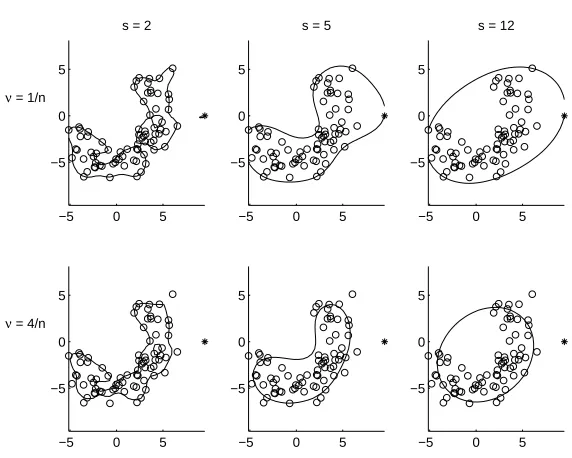
Figure 1: Decision boundaries of a simple 2-dimensional dataset, with different choices ofs
andν.
One intuitive parameter for the user is the fraction of the target objects which can be rejected by the description, fT−.Assume the user is satisfied with an error of 5% on the
target set.Then, one parameter (sorν) can be optimized, using estimate (6), such that 5% of the training objects become support vector.The SVDD will then have approximately
fT−= 0.05.Unfortunately, this will not uniquely define both parameters sandν, but just
In Figure 1 the decision boundaries of the SVDD for different choices of s and ν are shown for an artificial, 2-dimensional banana-shaped target set.The Figure shows that for smaller s, small details in the data are followed.On the other hand, whens is very large (in the order of the size of the complete dataset), only a spherical solution is found (for
s→ ∞the rigid hypersphere solution is obtained, (as shown in Tax and Duin, 1999).For
ν = 0 (C =∞) no target objects are allowed outside the description.All objects, including the remote object at (10,0), are accepted.When ν = 14 about one quarter of the target data can be outside the description.When enough data is available, a more robust estimate of the boundary is obtained.In general, when s is large and ν is small, a spacious data description is obtained.
For this 2-dimensional dataset it is possible to judge the boundary visually and to pick reasonable values for s and ν.For higher dimensional data this is not possible.In these cases other measures have to be invented to judge the quality of the description.For a good data description, we have two requirements: (1) a low target rejection rate fT− and (2) a
low outlier acceptance rate fO+.When we are only given examples of the target set, the first term can be estimated by the number of support vectors that we obtain as a solution of Lagrangian (9).
Minimizing just the error on the target set, fT−, is not sufficient.The solution would
be to accept the complete feature space.To estimate the outlier acceptance rate without example outliers, we have to assume an outlier distribution.When we assume the outliers are uniformly distributed in the part of the feature space we are interested in, we should minimize the volume which the description occupies.To minimize this, we have to estimate the volume of the description.This can be done by creating a large set of (artificial) outlier objects around the target dataset.When these outliers are uniformly distributed, the fraction of the outliers that is accepted, gives an estimate of the volume of the data description with respect to the volume of the outlier distribution.
Unfortunately, this procedure may become very expensive in high dimensional feature spaces.Assume that the target set is distributed in a hypercube with edges of unit length and that the outliers come from a hypercube with 10% larger edges (that means edges of length 1.1).In 10 dimensions the outlier distribution has 2.6 times the volume of the target set, but in 20-D this is already more than 3000 times! When data is generated in this outlier distribution, the chance that one of them falls in the target set, is about 0.3%.Of course, the target data can have different shapes, but it will always hold that the volumes of the target and outlier set will diverge with increasing dimensionality of the data.
For high dimensional data it is therefore essential that the outliers are tightly distributed (in and) around the target class to avoid that for the estimation of the target volume, a very high fraction of test outliers will be rejected and no confident target volume estimation can be made.It would be very easy to create objects uniformly from a hyperblock in d
dimensions, but it is not very likely that this distribution will fit very tightly around the target class.Many outlier objects will be generated in the corners of the box instead of into the data description.In this paper we propose to use the rigid hypersphere solution from formula (2).We hope this will fit tighter around the target set than the hyperbox.
description.We can now define the error for a one-class classifier:
Λ(s, ν) =λ#SV
N + (1−λ)
#outlier objects accepted #outlier objects =λ
#SV
N + (1−λ)fO+ (12)
where a new parameter λis introduced.Using this formula, we can optimize bothsand ν
to get minimum Λ.When we takeλ= 12, errors on the fraction of target and outlier objects are weighted equally.In the optimal solution, the fraction of target objects that is rejected, is equal to the volume fraction of the outlier area which is occupied by the target set.
Finally, generating samples which are uniformly distributed in a d-dimensional hyper-sphere is not easy.In the next section we propose a method to do this.
4. Generating samples uniformly from a hypersphere
Although a uniform hyperspherical outlier distribution might fit tighter around the tar-get class than a hyperbox distribution, it is not trivial to draw objects from a uniform hyperspherical distribution (Luban, M. and Staunton, L.P., 1988). Our key idea for the generation of these samples, is to use a d-dimensional Gaussian distribution.The direction of the object vectors from the origin will not be changed, but we rescale the norm of the object vectors.The generation is in several steps:
1.Generate datax from Gaussian distribution (with zero mean and unit variance),
x∼ N(0,1)
2.Calculate the squared Euclidean distance from each sample to the origin, r2.This squared distance is distributed as χ2 with ddegrees of freedom (Ullman, 1978).
r2 =x2
3.Use the cumulative distribution of χ2d, Xd2, to transform the r2 distribution in a uniform distribution between 0 and 1.This results in a uniform distribution of ρ2:
ρ2 =Xd2(r2) =Xd2(x2)
4.Rescaleρ2 by r = (ρ2)2d such thatr is distributed asr ∼rdforr between 0 and 1.
r=ρ22d =X2
d(x2)
2 d
5.Rescale all objectsx with this factor:
x= r xx
Given this outlier generation algorithm, it is possible to train a conventional classifier on these two classes.Although it is possible, one has to be careful.One has to generate enough artificial data to have objects around the target class in all feature directions. Second, one has to use a classifier which is local, i.e. a classifier which will generate a closed boundary around the target class and which will not classify remote objects as target objects.Finally, the classifier should be robust against large class-overlap, because by this method of generation of outlier objects, it cannot be avoided that outliers are generated within the target distribution.Even worse, because it is likely that a large set of outliers has to be generated for a good coverage over the target class, the two classes will be very imbalanced.Still the classifier should have small error on the target class (which is the only ’real’ data we have) and therefore the classifier should also be able to handle the difference in significance of the target and outlier objects.
5. Experiments
Given the error (12) and the possibility of efficiently generating outlier objects around the target data (and a value forλ!), we are able to optimize the free parameterssandν in the SVDD (with error (9) and evaluation formula (10)).In this section we want to investigate if the optimization of (12) results in reasonable values forsandν.In all cases we will optimize such that an equal fraction of the target and outlier objects is erroneously classified, which means we will useλ= 12.At the end of this section we will check if the classification results are reasonable, which means comparable with a data description using a density estimator.
5.1 Artificial example
In Section 3 we showed a simple banana-shaped dataset which contained one clear outlier at (10,0).Using this dataset, we generate 1000 outlier objects.We find simultaneouslys
and ν by minimizing error (12) (using a Matlab optimization routine) and we obtain the final data description.
−6 −4 −2 0 2 4 6 8 10 −8
−6 −4 −2 0 2 4 6
−4 −2 0 2 4 6 8
−6 −4 −2 0 2 4
The results are shown in Figure 2.The left subplot shows the artificial outlier data generated around the banana-shaped target set.In the right subplot the decision boundary for the SVDD with the optimized s and ν is shown.Note that we fitted the hypersphere to the training data.It can easily happen that the testing data is distributed somewhat around the training data and that therefore the hypersphere does not cover the testing set completely.Without using the testset it is not possible to find this out and we ignore this problem in this paper.
Because the errors for the target and outlier objects are equally weighted, the boundary of the dataset is not exactly around the data, but a fraction of the target data is rejected. On the other hand, the data description gives a good impression of the shape of the data. When the error on the target set should be smaller, the λin formula (12) can be adapted, or the threshold value (the right term in inequality (10)) can be changed.
5.2 Handwritten digits
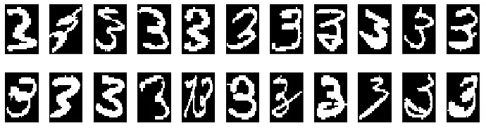
Figure 3: Testing target objects rejected by the data description.
To see if we can find outlier objects in a real world dataset, we trained a SVDD on a handwritten digits dataset (the Concordia dataset, which is also used, for instance, by Cho, 1996).This dataset contains handwritten digits (size 32×32), with 400 objects per class in a training set and 200 objects per class in a testing set.The data dimensionality was reduced from 1024 to about 30 using PCA, retaining 75% of the variance in the data. An SVDD was trained on the class representing the threes.The s and ν were optimized simultaneously by minimizing error (12) (λ= 12) using 100,000 artificially generated outlier objects (this large amount of outlier objects was necessary in order to obtain a reasonable confident estimate of the target class volume).
The SVDD was tested on the 200 testing handwritten threes.In Figure 3 the test objects are shown, which are rejected by the SVDD.From the 400 training objects 11% became support vector (αi>0).This fraction corresponds well with the error on the test set, where 24 of the 200 testing objects are rejected, i.e.an error of 12%.Surprisingly, some reasonable threes are rejected (the upper left three, for instance), but also a real segmentation error was detected (the thirteen in the lower left).Note that only information about the target class is used, and that no extra preprocessing was done (except for using 75% PCA).
Figure 4: Artificial objects (images of handwritten threes) generated from a box-shaped distribution around the target set (left subplot) and from a spherical-shaped distribution (right subplot).
from the spherical distribution.Although the images of both distributions are not ’crisp’ (caused by the PCA), the images from the box-distribution have backgrounds with very different gray values.This indicates that the images are distributed in (relative) remote parts in the feature space.The images from the spherical outlier distribution are closer to the real training images, especially considering the background which is now dark.
In this experiment it is even harder than in the 2-dimensional example, to judge if these results are good.Here no ground truth is available, i.e.an object is a genuine three, or an outlier three.In the next section we investigate an example where ground truth is available.
5.3 Texture segmentation
1 2 3
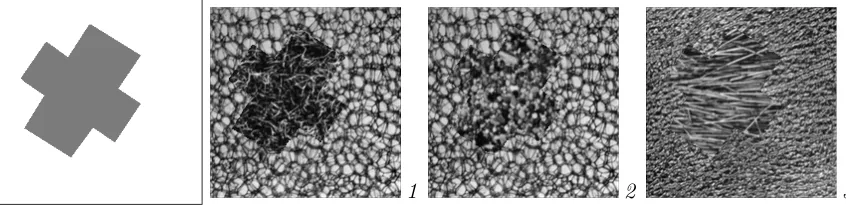
Figure 5: Texture segmentation.The texture in the cross shaped region in the middle is used as target class (left figure).The next three images are examples of textures used.
texture images with varying classification complexity are shown (next subplots).The cross-shaped, dark area contains the target texture, all other pixels are per definition outlier objects.To classify a pixel from the image, an image-patch containing 16×16 = 256 pixels is drawn around this pixel.Therefore, an object (one pixel) is characterized by a 256-dimensional feature vector.
In the experiments, the SVDD is trained on a training set, which is sampled from the complete target region.400 objects are used for training.A few outliers can be in the training set, because when a patch in the neighborhood of the boundary of the target class is used, a part of the outlier texture can be included in the patch.
We compare the results of the SVDD where we (1) set manually the fraction of objects that is on the boundary and outside the boundary, and (2) where we just optimize formula (12).When we manually set the parameters, we setC to a prespecified fraction of objects which isoutside the description, according to Equation (11).Objects outside the boundary automatically have αi = C.We will use ν = 0.0,0.1 and 0.2.The width parameter
s is optimized such that a prespecified fraction of the objects will be on the boundary. This means that the Lagrange multiplier αi corresponding to the support vector xi has 0< αi < C.The parameter s can be optimized to obtain this prespecified fraction of the training data on the boundary (we will use the values 0.0,0.05,0.1 and 0.2), but this fraction is not an intuitive quantity.Without knowledge about the complexity of the boundary of the dataset, just several values for this fraction have to be tried.The performance on some test data should be used to decide for the final setting.
In the automatic optimization the number of artificial outlier objects is set to 100,000. We use λ= 12.Because 400 target and 100,000 outlier objects are used, the errors on the target and the outlier data are not equally weighted in error (12).An error on the target data is weighted 2500 times heavier than an error on an outlier object in the optimization of the error (12).
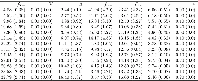
Table 1: Performances on image1 using a trainingset of 400 patches (size 16×16).160 fea-tures are used.Results are averaged over 5 runs and multiplied by 100.Numbers in brackets give the standard deviation.
fT− V Λ fO+ Etot s ν
To test the data descriptions, we will use both the artificially created examples and the pixels from the original texture images (or actually a subsampled version).The second type of outliers will be called the ’true’ outliers.Because the outlier data in the images is not uniformly distributed in the feature space, it can be expected that the optimization of error (12) will give suboptimal results with respect to the ’true’ outliers.This deviation can never be detected without the use of negative examples.When these negative examples are not available, it is only hoped that by using the artificial, uniformly distributed outliers, a reasonable solution is obtained.
The results for image 1 are shown in Table 1.The first row gives the results for the automatic optimization, the next 12 rows give the performances for several manual settings (optimizing s and ν for specific fractions of the target set on and outside the boundary). The first columnfT−shows the fraction of the target set which is rejected (estimated on all
target pixels) times 100.A value 4.88 means that about 5% of the target objects is rejected by the data description.The numbers in brackets show the standard variation over 5 runs. The second columnV shows the fraction of artificial outliers which is accepted.The third column λthen gives the average error over the target and the artificial outliers, Etot.The fourth columnfO+ shows the fraction of outlier objects which is accepted (again using all outlier pixels from a subsampled image).Note that we test on the ’real’ outlier objects from the image, and that we do not use the artificial negative examples.The fifth column Etot shows the average of the target and outlier error (column 1 and 4).The two last columns show the sand ν respectively.
In the first experiment the data was mapped from 256 to 160 dimensions, retaining 99% of the variance in the data.This is still a very high dimensionality to generate outlier data in.It can be observed in the Table 1 that in this high dimensional feature space the optimization of error (12) results in a very rough approximation of the data.A very small number of artificial outlier objects falls within the sphere: the column ’V’ shows all values of 0.0, indicating that (almost) all objects fall outside the description.Therefore there is almost no force to minimize the volume of the description and the width parameter
s in the data description is very large (see the fourth column).Practically, a hypersphere solution is found.The number of target objects that is rejected is therefore very low (first column) but also a large fraction of the outlier objects is accepted (second column).From this experiment we can conclude that we should decrease the dimensionality of the feature space to find a better description.
In Table 2 the results on the same image is shown, only here the dimensionality of the feature space was reduced from 265 to 35 dimensions (retaining about 75% of the variance). The values in the second column now show that we are able to estimate the volume occupied by the target set.The estimated volumes are bigger now (although they are still pretty small) and the values forsand ν can be determined with higher confidence.
Table 2: Performances on image1 using a trainingset of 400 patches.35 features are used. Results are averaged over 5 runs and multiplied by 100.Numbers in brackets give the standard deviation.
fT− V Λ fO+ Etot s ν
2.96 (0.94) 1.44 (0.45) 2.20 (0.39) 39.98 (7.49) 21.47 (3.37) 4.67 (0.30) 0.00 (0.0) 2.35 (0.26) 6.10 (2.79) 4.23 (1.30) 46.24 (6.31) 24.29 (3.12) 5.53 (0.31) 0.00 (0.0) 6.89 (1.77) 0.53 (0.47) 3.71 (0.78) 16.68 (7.75) 11.79 (3.03) 5.69 (0.39) 0.10 (0.0) 15.56 (0.98) 0.01 (0.01) 7.78 (0.49) 2.20 (0.54) 8.88 (0.40) 5.17 (0.46) 0.20 (0.0) 4.35 (0.72) 0.60 (0.50) 2.47 (0.32) 32.52 (6.96) 18.44 (3.24) 3.87 (0.26) 0.00 (0.0) 8.36 (1.21) 0.14 (0.14) 4.25 (0.55) 12.62 (4.48) 10.49 (1.72) 3.63 (0.53) 0.10 (0.0) 14.82 (1.64) 0.00 (0.00) 7.41 (0.82) 2.19 (0.91) 8.50 (0.37) 2.70 (0.10) 0.20 (0.0) 10.58 (1.21) 0.01 (0.01) 5.29 (0.61) 8.24 (3.37) 9.41 (1.13) 2.64 (0.06) 0.00 (0.0) 10.86 (1.27) 0.00 (0.00) 5.43 (0.63) 6.80 (1.60) 8.83 (0.67) 2.56 (0.03) 0.10 (0.0) 18.16 (1.78) 0.00 (0.00) 9.08 (0.89) 1.03 (1.14) 9.60 (0.38) 2.26 (0.04) 0.20 (0.0) 15.16 (0.79) 0.00 (0.00) 7.58 (0.39) 1.76 (0.44) 8.46 (0.53) 2.23 (0.02) 0.00 (0.0) 15.54 (1.41) 0.00 (0.00) 7.77 (0.70) 2.31 (1.04) 8.93 (0.38) 2.23 (0.04) 0.10 (0.0) 20.90 (1.33) 0.00 (0.00) 10.45 (0.66) 0.54 (0.32) 10.72 (0.61) 2.06 (0.02) 0.20 (0.0)
Table 3: Performances on image1 using a trainingset of 400 patches.12 features are used. Results are averaged over 5 runs and multiplied by 100.Numbers in brackets give the standard deviation.
fT− V Λ fO+ Etot s ν
6.54 (0.84) 4.99 (1.79) 5.76 (0.76) 15.61 (5.74) 11.08 (2.83) 2.87 (0.26) 0.01 (0.0) 1.27 (0.36) 36.61 (7.91) 18.94 (3.98) 53.84 (8.54) 27.56 (4.19) 5.48 (0.33) 0.00 (0.0) 8.03 (1.24) 6.88 (2.59) 7.46 (0.72) 13.56 (5.29) 10.80 (2.11) 4.80 (0.69) 0.10 (0.0) 16.98 (1.17) 1.86 (0.49) 9.42 (0.42) 2.14 (0.43) 9.56 (0.49) 4.94 (0.58) 0.20 (0.0) 5.61 (1.44) 4.73 (1.06) 5.17 (0.61) 23.80 (6.26) 14.70 (2.50) 2.71 (0.14) 0.00 (0.0) 9.29 (1.34) 2.18 (0.79) 5.73 (0.34) 9.70 (3.55) 9.50 (1.17) 2.39 (0.12) 0.10 (0.0) 16.38 (1.05) 0.57 (0.20) 8.47 (0.43) 2.44 (0.47) 9.41 (0.60) 2.10 (0.04) 0.20 (0.0) 9.86 (2.32) 1.22 (0.77) 5.54 (0.80) 8.83 (7.97) 9.34 (3.06) 2.11 (0.24) 0.00 (0.0) 11.03 (2.49) 1.13 (0.97) 6.08 (0.90) 6.94 (4.72) 8.98 (1.65) 2.05 (0.25) 0.10 (0.0) 19.93 (1.52) 0.23 (0.05) 10.08 (0.74) 0.64 (0.15) 10.29 (0.71) 1.67 (0.03) 0.20 (0.0) 17.66 (1.67) 0.32 (0.11) 8.99 (0.82) 1.37 (0.69) 9.51 (0.61) 1.63 (0.04) 0.00 (0.0) 20.06 (0.63) 0.23 (0.08) 10.15 (0.31) 1.00 (0.52) 10.53 (0.31) 1.61 (0.01) 0.10 (0.0) 24.18 (0.95) 0.10 (0.02) 12.14 (0.47) 0.40 (0.26) 12.29 (0.40) 1.52 (0.02) 0.20 (0.0)
’true’ outlier set.It appears that up to 10D no significant extra overlap between the classes is introduced.This is visible when we compare the results from Table 2 and 3.When we reject 8.36% of the target objects in 35D (fT−in Table 2), about 12.6% of the ’true’ outlier
reject 8.03% of the target data, and accept 13.6% of the outliers.Considering the variance on the outcomes, this is just a small increase.
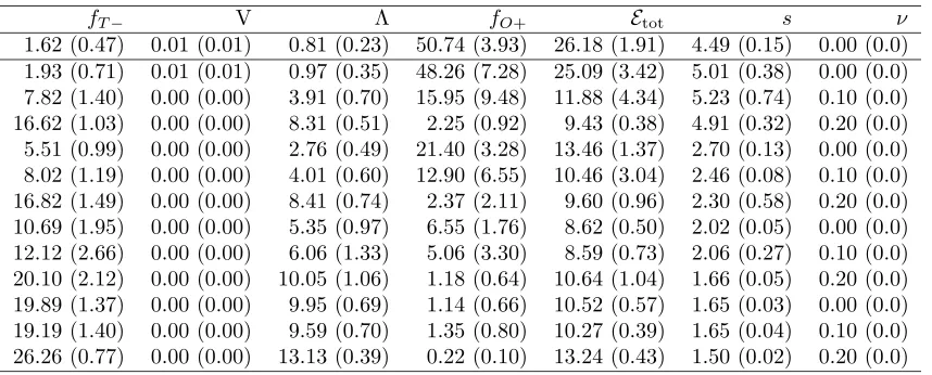
Table 4: Performances on image1 using a trainingset of 400 patches.Outliers are generated in a hyperbox, instead of in a hypersphere.12 features are used.Results are averaged over 5 runs and multiplied by 100.Numbers in brackets give the standard deviation.
fT− V Λ fO+ Etot s ν
1.62 (0.47) 0.01 (0.01) 0.81 (0.23) 50.74 (3.93) 26.18 (1.91) 4.49 (0.15) 0.00 (0.0) 1.93 (0.71) 0.01 (0.01) 0.97 (0.35) 48.26 (7.28) 25.09 (3.42) 5.01 (0.38) 0.00 (0.0) 7.82 (1.40) 0.00 (0.00) 3.91 (0.70) 15.95 (9.48) 11.88 (4.34) 5.23 (0.74) 0.10 (0.0) 16.62 (1.03) 0.00 (0.00) 8.31 (0.51) 2.25 (0.92) 9.43 (0.38) 4.91 (0.32) 0.20 (0.0) 5.51 (0.99) 0.00 (0.00) 2.76 (0.49) 21.40 (3.28) 13.46 (1.37) 2.70 (0.13) 0.00 (0.0) 8.02 (1.19) 0.00 (0.00) 4.01 (0.60) 12.90 (6.55) 10.46 (3.04) 2.46 (0.08) 0.10 (0.0) 16.82 (1.49) 0.00 (0.00) 8.41 (0.74) 2.37 (2.11) 9.60 (0.96) 2.30 (0.58) 0.20 (0.0) 10.69 (1.95) 0.00 (0.00) 5.35 (0.97) 6.55 (1.76) 8.62 (0.50) 2.02 (0.05) 0.00 (0.0) 12.12 (2.66) 0.00 (0.00) 6.06 (1.33) 5.06 (3.30) 8.59 (0.73) 2.06 (0.27) 0.10 (0.0) 20.10 (2.12) 0.00 (0.00) 10.05 (1.06) 1.18 (0.64) 10.64 (1.04) 1.66 (0.05) 0.20 (0.0) 19.89 (1.37) 0.00 (0.00) 9.95 (0.69) 1.14 (0.66) 10.52 (0.57) 1.65 (0.03) 0.00 (0.0) 19.19 (1.40) 0.00 (0.00) 9.59 (0.70) 1.35 (0.80) 10.27 (0.39) 1.65 (0.04) 0.10 (0.0) 26.26 (0.77) 0.00 (0.00) 13.13 (0.39) 0.22 (0.10) 13.24 (0.43) 1.50 (0.02) 0.20 (0.0)
In Table 4 the last experiment is repeated, but now artificial outliers are generated not in a hypersphere, but in a hyperbox.The values in the second columnV show that the volume fraction, occupied by the target set is very small, even for this 12-dimensional feature space. In most cases, the number of artificial outlier objects which is accepted is very low, and the parameters sand ν are optimized such that a very broad data description is obtained (i.e. very large s and very small ν, see Section 3).This shows that the hyperspherical outlier distribution fits tighter around the target set, and provides better volume estimates than the hyperbox approach.
In Table 5 the results are shown for image 2, and similar results are obtained.In this case there is more overlap between the target and outlier class.In this target dataset it can be observed that some outliers are present.While in image1 in almost all casesν was optimized to (almost) zero, in image 2 about 10% of the target objects is rejected.
Table 5: Performances on image2 using a trainingset of 400 patches (size 16×16).10 fea-tures are used.Results are averaged over 5 runs and multiplied by 100.Numbers in brackets give the standard deviation.
fT− fO+ Etot s ν
9.66 (0.91) 48.52 (2.36) 29.09 (1.13) 2.68 (0.42) 0.06 (0.05) 1.98 (1.22) 68.10 (4.01) 35.04 (1.49) 5.02 (0.54) 0.00 (0.00) 7.97 (2.16) 52.94 (8.43) 30.45 (3.31) 5.04 (0.95) 0.10 (0.00) 14.66 (1.24) 37.72 (5.49) 26.19 (2.18) 5.05 (0.49) 0.20 (0.00) 4.88 (2.03) 57.93 (5.46) 31.41 (1.85) 3.34 (0.44) 0.00 (0.00) 10.12 (0.33) 47.31 (3.65) 28.72 (1.93) 2.72 (0.15) 0.10 (0.00) 19.03 (1.88) 31.79 (4.88) 25.41 (1.63) 2.28 (0.05) 0.20 (0.00) 13.30 (1.30) 43.30 (3.48) 28.30 (1.68) 2.17 (0.06) 0.00 (0.00) 14.70 (1.60) 41.02 (4.43) 27.86 (1.80) 2.12 (0.05) 0.10 (0.00) 21.65 (1.19) 30.22 (3.01) 25.93 (1.78) 1.92 (0.01) 0.20 (0.00) 20.57 (1.39) 31.16 (1.94) 25.86 (1.35) 1.86 (0.03) 0.00 (0.00) 21.26 (1.45) 30.43 (2.67) 25.84 (1.48) 1.84 (0.03) 0.10 (0.00) 25.01 (6.16) 28.26 (8.50) 26.64 (1.77) 1.91 (0.30) 0.20 (0.00)
0 0.2 0.4 0.6 0.8 1 0
0.05 0.1 0.15 0.2 0.25 0.3 0.35 0.4 0.45 0.5
λ
fraction
target outlier
0 0.2 0.4 0.6 0.8 1 0
0.2 0.4 0.6 0.8 1
λ
fraction
target outlier
Figure 6: Performance on the target and outlier set,fT− and fO+, for varying λ.Left the results for image1 is shown, right for image3.Results are averaged over 5 runs.
In the right subplot the result for image3 is shown.Here the performance on the outlier class is very poor.For most values ofλless than 20% of the target data is rejected, but all outlier data is accepted.This indicates that the target data might be distributed around the outlier data.This can be seen in the next figure.
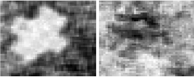
Figure 7: Output of SVDD with optimized s and ν for (left) image 1 and (right) image 3, λ = 12.A light grayvalue indicates that the pixel is near the center a of the SVDD hypersphere (and thus classified as target object by the SVDD).
as target object by the SVDD).Thesandν are optimized by minimizing error (12) (results of image 2 is comparable to image 1).The results on image 1 show that the target class can be distinguished well from the background texture.For image3 on the other hand, it appears that the data description on the target class, gives an even better description for the outlier class! It appears that the outlier class is clustered much tighter and lies within the target class.This can be explained from the textures in subplot 3 in Figure 5.They show that the outlier class consists of particles which are shorter versions of the straws in the target class.The outlier class is therefore a subcluster in the target class.2
Although it is not our prime concern to find the ultimate performance on this dataset in this paper, the performance should still be at least comparable with other methods. To investigate if the solutions obtained by the SVDD are reasonable, a comparison with a simple density estimator is made.We trained a Mixture of Gaussians model (Bishop, 1995) on the target set (using the conventional EM algorithm (Dempster et al., 1977)). The number of clusters k was found by minimizing the Akaike Information Criterion (Akaike, 1974).In most cases one or two minima for the number of clusters could be identified.Given a mixture, the threshold on the density was optimized by minimizing an error comparable with definition (12):
Λ(θ) =λ#target objects rejected
#target objects + (1−λ)
#outlier objects accepted #outlier objects
When λ = 12 was used, extremely poor results were obtained, therefore λ = 100400,000 was chosen.
In Table 6 the results of the classification by both the SVDD and the Mixture of Gaus-sians is shown for the three images.The results show that for the Mixture of GausGaus-sians the fT− is lower and on the other hand that the covered volume in the feature space is
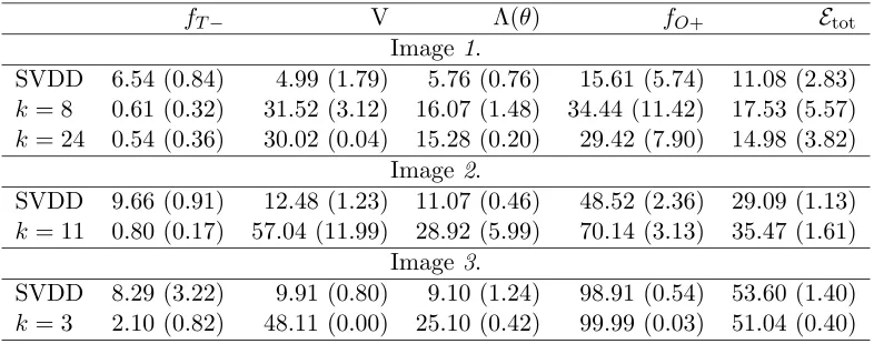
Table 6: Performances of the Mixture of Gaussians (with different number of clusters, k) compared with the SVDD on the three images.A trainingset of 400 patches is used (size 16×16).Results are averaged over 5 runs and multiplied by 100.Numbers in brackets give the standard deviation.
fT− V Λ(θ) fO+ Etot
Image 1.
SVDD 6.54 (0.84) 4.99 (1.79) 5.76 (0.76) 15.61 (5.74) 11.08 (2.83)
k= 8 0.61 (0.32) 31.52 (3.12) 16.07 (1.48) 34.44 (11.42) 17.53 (5.57)
k= 24 0.54 (0.36) 30.02 (0.04) 15.28 (0.20) 29.42 (7.90) 14.98 (3.82) Image 2.
SVDD 9.66 (0.91) 12.48 (1.23) 11.07 (0.46) 48.52 (2.36) 29.09 (1.13)
k= 11 0.80 (0.17) 57.04 (11.99) 28.92 (5.99) 70.14 (3.13) 35.47 (1.61) Image 3.
SVDD 8.29 (3.22) 9.91 (0.80) 9.10 (1.24) 98.91 (0.54) 53.60 (1.40)
k= 3 2.10 (0.82) 48.11 (0.00) 25.10 (0.42) 99.99 (0.03) 51.04 (0.40)
significantly larger.Therefore, also the fO+ tends to be much larger than for the SVDD. The Mixture of Gaussians appears to fit a much broader boundary around the data.This is also visible in the results of image 1, where for a high number of clusters, k= 24, better results are obtained than for a smaller number of clusters, k= 8.As it is to be expected, both methods collapse on the data from the last image;fO+ is almost 100% in both cases. This is shown in the last two rows of Table 6.
6. Conclusion
In one-class classification we assume that we have examples from just one class, called the target class and that all other possible objects, per definition the outlier objects, are uniformly distributed.In this paper we used the support vector data description (SVDD) to separate the target class of data from the rest of the feature space.It models a hypersphere around the target data with minimal volume.Analogous to the method of Vapnik (1998), it is possible to replace the inner products by kernel functions which gives a much more flexible method.In this paper a Gaussian kernel is used.
In this basic form, the user has to supply two parameters, indicating the important scale in the data, s, and the fraction of objects which is expected to be outlier, or which are not representative for the description of the data, ν.When the user supplies the error which is allowed on the target class, one parameter can be optimized.To optimize the second parameter, we choose to minimize the chance of accepting outliers.An error criterion (formula (12)) is defined which contains the fraction of the target objects we want to accept and the volume of the data description in the feature space.The value of the two parameters
sand ν is optimized by minimizing this error.
dimensional feature spaces.When a hyperbox is defined around the target set, the vol-ume covered by the target class and by the hyperbox diverge for high dimensional feature spaces.The result is that outlier objects which are drawn or generated from a hyperbox, are accepted by the one-class classifier with very low probability (most objects are created in the ’corners’ of the hyperbox).To make this procedure applicable in high dimensional feature spaces, the volume in which the artificial outliers are generated, has to fit as tight as possible around the target class.We propose to generate outliers uniformly in a hyper-sphere.This is done by transforming objects generated from a Gaussian distribution.Only the distribution of the norm of the vectors is transformed and the direction of the vectors is constant.
Experiments indicate that, using these artificial outliers from a hyperspherical distri-bution, values for s and ν can be obtained with higher efficiency than from a hyperbox distribution.Only for very high dimensionalities the required number of artificial outliers becomes huge.Then it is very hard to get a confident estimate of the target volume due to the large difference in volume of the target and outlier class.Experiments suggest that up to 30 dimensions, the procedure to artificially generate outliers in a hypersphere is feasible. Finally, optimizing sand ν using the artificial outliers does not guarantee that the per-formance on ’real’ outlier objects will be good.In some cases the target class is represented such that it is scattered over the complete feature space.In this case it cannot be expected that a one-class classifier can distinguish between target and outlier objects.Only when example outliers are available, this can be checked.
Acknowledgments
This work was partly supported by the Foundation for Applied Sciences (STW) and the Dutch Organization for Scientific Research (NWO).
References
H.Akaike. A new look at the statistical model identification. IEEE Transactions on Automatic Control, AC–19:716–723, 1974.
C.M. Bishop. Neural Networks for Pattern Recognition.Oxford University Press, Walton Street, Oxford OX2 6DP, 1995.
C.J.C. Burges. A tutorial on support vector machines for pattern recognition. Data Mining and Knowledge Discovery, 2(2), 1998.
Sung-Bae Cho.Recognition of unconstrained handwritten numerals by doubly self-organizing neural network.In International Cconference on Pattern Recognition, 1996.
N.M.Dempster, A.P.Laird, and D.B.Rubin. Maximum likelihood from incomplete data via the EM algorithm. J. R. Statist. Soc. B, 39:185–197, 1977.
M.R. Moya, M.W. Koch, and L.D. Hostetler. One-class classifier networks for target recog-nition applications.In Proceedings world congress on neural networks, pages 797–801, Portland, OR, 1993.International Neural Network Society.
B.Sch¨olkopf, P.Bartlett, A.J.Smola, and R.Williamson. Shrinking the tube: A new support vector regression algorithm. M.S.Kearns, S.A.Solla, and D.A.Cohn, editors, Advances in Neural Information Processing Systems, 1999.
B.Sch¨olkopf, C.Burges, and V.Vapnik.Extracting support data for a given task.In U.M. Fayyad and R.Uthurusamy, editors, Proc. of first international conference on knowledge discovery and data mining, pages 252–257, Menlo Park, CA, 1995.AAAI Press.
B.Sch¨olkopf, R.C.Williamson, A.Smola, and J.Shawe-Taylor. SV estimation of a distri-bution’s support.In Advances in Neural Information Processing Systems, 1999.
D.M.J. Tax. One-class classification.PhD thesis, Delft University of Technology, http://www.ph.tn.tudelft.nl/˜davidt/thesis.pdf, June 2001.
D.M.J. Tax and R.P.W Duin. Support vector domain description. Pattern Recognition Letters, 20(11-13):1191–1199, December 1999.
N.R. Ullman. Elementary statistics, an applied approach.Wiley and Sons, 1978.