Model Predictive Control of Distributed Energy Resources with Predictive Set-Points for Grid-Connected Operation

AUT J. Elec. Eng., 50(2) (2018) 109-120 DOI: 10.22060/eej.2018.14303.5217

Model Predictive Control of Distributed Energy Resources with Predictive Set-Points

for Grid-Connected Operation

A. Saleh*_{, A. Deihimi}

Electrical Engineering Department, Bu-Ali Sina University, Hamedan, Iran

ABSTRACT: This paper proposes an MPC - based (model predictive control) scheme to control active and reactive powers of DERs (distributed energy resources) in a grid - connected mode (either through a bus with its associated loads as a PCC (point of common coupling) or an MG (micro - grid)). DER may be a DG (distributed generation) or an ESS (energy storage system). In the proposed scheme, the set - points provided to MPC are forecast for future instances by a linear extrapolation to gain smooth active and reactive power exchange under various loading conditions (e.g. balanced / imbalanced, nonlinear and dynamic loading) and voltage imbalance imposed by the upstream grid. In this scheme active and reactive power control change to current control and the references of the currents are forecast. The stability of the proposed control scheme is analyzed and discussed. The effectiveness of the proposed scheme is demonstrated by extensive time - domain simulations using PSCAD / EMTDC for various conditions (various loads, voltage imbalance, parallel operation with other DGs, parameter uncertainties and measurement noises) in several case studies. Comparing the obtained results with those of the two other schemes (PI - based and convectional MPC) shows the superiority of the proposed scheme.

Review History:

Received: 9 April 2018 Revised: 10 June 2018 Accepted: 4 September 2018 Available Online: 1 October 2018

Keywords:

Distributed Energy Resource Micro-Grid

Grid-Connected Operation Model Predictive Control Predictive Set-Points

1- Introduction

MGs (micro-grids) which consist of DERs (distributed

energy resources) (DGs (distributed generations) and ESSs

(energy storage systems)) and loads, which are electrically

connected to each other, are conceived as a small grid [1], [2]. As DGs, WT (wind turbine) and PV (photovoltaic array) are

suitable to apply in MGs,because of their geographical small

size and more scalable than conventional power plants. Also, conventional generators (diesel and gas fueled generators) are used into MGs [3]. When WT and PV are used as the major DGs in the MGs, since energy sources of them have intermittent and stochastic nature, energy storages, as ESSs, play an important role in the MGs to support renewable power penetrations [4]. MG can operate grid-connected or islanded. In grid-connected operation, MG is connected to the main grid at the PCC (point of common coupling) and voltage and frequency are dictated by the main grid. In this operation mode DERs must properly exchange active and reactive powers that are deduced by operation management [5] in the various conditions e.g. imbalanced/nonlinear load

and imposed voltage imbalance. In reference [6], a

current-controlled real-/reactive-power controller is developed where conventional PI-based is used as the main controller. This control scheme is designed for inverter-based renewable sources which are connected to a balanced grid and has no proper performance under unmoral conditions. References

[7] and [8] proposed direct power control strategies based

on sliding mode control method under voltage unbalancing of main grid, but imbalanced/nonlinear load conditions are

not demonstrated. Two control schemes based on adaptive

Lyapunov function and sliding mode method in [9] are used to compensate the negative-sequence current components

caused by unbalanced loads in some part of the MG and directly regulate the positive-sequence active and reactive

power injected by DGs to the MG, respectively. Reference [10]

proposed direct Lyapunov control method to control DGs in

a grid connected MG with nonlinear loads. The used method in [11] is developed to improve grid-connected operation of inverter-based renewable resources under grid-impedance uncertainties. The proposed control scheme in [12] utilizes PI current controller for a WT to control delivered power to distributed grid under existence nonlinear loads.

In recent years, MPC (model predictive control) has found many applications in power electronics and other industrial

fields [13-23]. MPC is greatly suitable for the control of

power converters due to its fast dynamic response, easy inclusion of nonlinearities and flexibility to include system requirements in controller design [19]. One of the solutions to control the grid-connected electronically-interfaced DGs was proposed in [13] where a direct power control scheme based on MPC was designed and examined for normal conditions,

e.g. balanced load and grid voltage and imbalanced/nonlinear

load and voltage imbalance conditions were not considered.

Model predictive scheme was proposed in [14] to control active and reactive powers for a single WT connected to the main grid through an LC filter. This reference considered neither imbalanced/nonlinear load nor voltage imbalance conditions.

In view of the aforementioned previous works, the main controller of inverter-based DERs should be preferably designed insensitive to loading dynamics to give a robust transient and steady-state performance at various loading and bus voltage conditions under grid-connected operation. Moreover, the fast dynamic response of MPC along with its optimal dedicated design based on system requirements can be used to achieve better regulation of power exchange of

a DER with on-grid system. Hence, a control scheme based on MPC is proposed in this paper for the main controller of inverter-based DERs where set-points of the inverter currents are forecast for future times (against conventional method in design of MPC) to give a desired performance regardless of loading variations or bus voltage imbalance. The effectiveness of the proposed control scheme is demonstrated by time-domain simulation conducted in PSCAD/EMTDC.

This paper is organized as follows. In section 2, the considered multi-bus MG is described. Structure of used DERs in the MG and their main proposed controllers are developed in sections 3 and 4. Simulation results are discussed in section 5, and conclusion is given in section 6.

2- Multi-bus MG description

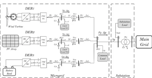
Fig.1 shows the single-line diagram of the considered multi-bus MG.

The MG consists of three inverter-based DER units which two of them are DGs and the other is ESS. DER1 is a WT, and DER2 is a PV array. WT and PV are main producers. The DER3 is a BT (battery bank) for storing extra energy produced by DGs or receiving from main grid in off-peak durations. The stored energy is used when DGs cannot provide power demand. Voltage of DER converter dc-link is regulated by its respective AC/DC or DC/DC converter at a desired voltage

(V_DC) as seen in Fig. 1, and the DER will deliver the necessary

power in such a way that maintains the power balance in the dc-link [22]. Thus the energy source/storage of each DER is replaced by an ideal DC voltage source [24]. Each DER is connected to its PC (point of connection) bus through an LC filter. Power exchange of each DER is occurred through a

step-up Y/Δ transformer. Transformers are paralleled to each

other at PCC (point of common coupling) through

interlink-lines modeled by series RL branches. PCC is connected to

20 KV main grid via a step-up Δ/Y transformer (as main

transformer) installed in substation. Three groups of loads are assumed that includes local load, common load and substation load. Local loads are connected to PC buses of DGs. This group (Fig.2) consists of balanced/imbalanced, nonlinear and dynamic motor loads. Common load which is a balanced load is connected to PCC. Substation load is connected to the low voltage side of the main transformer that can be balanced/ imbalanced load. Parameters of the DERs, MG, substation and main grid are given in Table 1.

Fig. 1. Single-line diagram of the considered multi-bus MG.

Table 1. DERs, MG, Substation and Main Grid parameters

Parameter Remark

DERs

Power

rating 10 Inverter

L_f 100

filter

C_f 500

R 1.5

V_DC 4 DC-link

f_s 6480 Switching frequency

Ts [µs] 10 Sampling time

Tr 0.612/4 (Y/Δ) Leakage reactance X=10%

Local Loads

R₁ 83

RL Local Load

L₁ 137

R₂ 50

RLC Local Load

L₂ 68

C₂ 13.55

R₃ 17 Imbalanced Local Load (phase a to ground- Tr: 0.612/0.184 (Δ /Y), X=10%)

L₃ 21.8

R₄ 700 _{Nonlinear Local Load (Tr:} 0.612/0.612 (Δ /Y), X=10%)

L₄ 20

Power

rating 0.8

Induction Machine Local Load

V_m 0.868

ω 377

R_r [pu] 0.0132 R_s [pu] 0.0184 L_m [pu] 3.8 L_lr [pu] 0.0223 L_ls [pu] 0.0223

MG

Z_l1 50+j37.70

Inter-link lines Impedance Z_l2 60+j45.24

Z_l3 55+j41.47

R_c 8300

RL Common Load

L_c 13700

Substation

Tr 4/20 (Δ /Y) Leakage reactance X=10%

R_sub 7 Imbalanced Substation Load (phase a to ground- Tr: 4/0.612 (Δ /Y), X=10%)

L_sub 20

Main Grid

V 20

3- DER and its main controller

A typical inverter-based DER along with its main controller is

shown in Fig. 3. The synchronous dq reference frame is used

for the control system while the PLL (phase locked loop) [25]

produces ρ as the angle between the rotating d-axis and the

stationary α-axis as well as ω as the angular frequency of PC

voltage. PC voltage v_oabc and ω are imposed by the upstream

grid.

The main controller regulates exchanged active and

reactive powers to their set-points (P_g*_{, Q}

g*). For DGs, Pg*

is determined by the MPPT (maximum power point tracker) algorithm [26-29], and for ESS, is deduced based on power balance as follow [5]:

(1)

WT PV BT loss load demand

P

+

P

+

P

=

P

+

P

+

P

P_WT, P_PV and P_BT are WT, PV and BT powers. P_loss, P_load and

P_demand are total loss of the MG network, total load in MG and demanded power by main grid.

Q_g* _{is provided by the MG operator that can be zero, negative}

or positive values [14]. The instantaneous active and reactive

powers P_g and Q_g are exchanged between DER and upstream

grid, calculated from output voltages and currents as bellow (2)

3

( ) ( ( ) ( ) ( ) ( ))

2

g od gd oq gq

P t = v t i t v t i t+

(3)

3

( ) ( ( ) ( ) ( ) ( ))

2

g od gq oq gd

Q t = −v t i t v t i t+

v_od and v_oq are dq components of the PC voltage.i_gd , and i_gq

are dq components of the interlink-line currents. With respect

to (2) and (3), one can deduce that [6]

(4)

* * *

2 2 2 2

( ) ( )

2 2

( ) ( ) ( )

3 ( ) ( ) 3 ( ) ( )

oq od

gd g g

od oq od oq

V t V t

i t P t Q t

V t V t V t V t

= +

+ +

(5)

* * *

2 2 2 2

( ) ( )

2 2

( ) ( ) ( )

3 ( ) ( ) 3 ( ) ( )

oq od

gq g g

od oq od oq

V t V t

i t P t Q t

V t V t V t V t

= −

+ +

where V_od and V_oq are signals obtained from filtering v_od

and v_oq respectively. i_gd* _{, and i}

gq* are set-points of igd and igq

respectively.v_od and v_oq are filtered in such a way that only

high frequency disturbances caused by inverter switching

can be removed. Thus, tracking the P_g* _{and Q}

g* are changed

to tracking the i_gd* _{and i}

gq*. In the next section the proposed

control scheme is described. 4- The proposed control scheme

4- 1- Controller construction

In this section, MPC [30] is used for the main controller

of an inverter-based DER to regulate i_gdand i_gqof the DER

connected to an on-grid system (Fig.3). Assume that a DER

is individually connected to a balanced main grid (v_od = dc

constant and v_oq = 0) and has no local load (i_Labc= 0). With

respect to Fig.3 [6]

(6) ( )

d gd i (t) i t=

(7)

( )

q gq f o

i (t) i t C v

=

+

ω

Therefore, in order to control i_gd(t) and i_gq(t), i_d(t) and i_q(t)

must be controlled. i_d(t) and i_q(t) are dq components of the

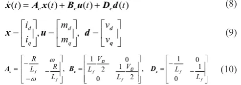
inverter currents. Thus state-space equations of the model can

be expressed as given in (8)-(10).

(8) ) ( ) ( ) ( )

(t A xt B ut Dd t

x = c + c + c

(9)       =       =       = oq od q d q d v v m m i i d u

x , ,

(10)         − − =           =         − − − = f f DC f D C f f f L L V L V L L R L R 1 0 0 1 , 2 10 02 1

, c c

c B D

A ω

ω

x, u and d are vectors of states, inputs and disturbances,

respectively. m_d and m_q are dq components of modulating

signals. Filter inductance and capacitance are denoted by

L_fand C_f, respectively. R models the ohmic loss of the filter

inductor and includes the effects of on-state resistance of switches. The states of the model are also assumed as the

Fig. 2. The collection of different load types connected to the PC of the DGs.

outputs of the model as given in (11) and (12) in order to limit the excursions of output currents of the inverter in design of MPC.

(11) )

( )

(t C x t

y = c

(12)       = 1 0 0 1 c C

Then, the discrete-time state-space equations are derived as

given in (13)-(15) using T_s as the sampling time.

(13) ) ( ) ( ) ( ) 1

(k m m k m k m k

m A x B u D d

x + = + +

(14) )

( )

(k Cmxm k

y =

(15)

1 1

, ( ) , ( ) ,

c s c s c s

A T A T A T

m m c c m c c m c

A ₌e B ₌A e− ₋I B D ₌A e− ₋I D C ₌C

Differences of the state-space equations in (13) are:

(16)

( 1) ( 1) ( ) ( ) ( ) ( )

m m m m m m m

x k x k x k A x k B u k D d k

∆ + = + − = ∆ + ∆ + ∆

∆x_m, ∆u and ∆d are differences of the states, inputs and

disturbances, respectively. If the sampling time is sufficiently

small, it can be assumed that the imposed voltages by the on-grid system have no large excursions during each time step and Δd(k)≈ 0 for k_i ≤ k ≤ k_i+N_c-1. Thus, the augmented state-space model is expressed as below:

(17)

( 1) ( ) ( )

X k+ =AX k + ∆B u k

(18)

( ) ( )

y k =CX k

(19)

[

]

( )

( ) m_{( )} , m , m ,

m m m m

A 0 B

x k

X k =_∆_{y k} _ A=__{C A I}_ B=_{C B } C= 0 I

     

The objective function that is optimized for MPC is: (20)

( ) (T ) T

s s

J = R Y Q R Y− − + ∆U R U∆

where

(21) 2

1 2

[ ( 1| ) ( | )] ( )

, ( ) _{( )} , ( ), ( ) _{( )} ( 1) p T

i i i p i i B

B

Np Np Np Nc

N

i _{dref i}

s i i

qref i

i c

Y y k k y k N k FX k U

CA CB 0 0

CAB CB 0

CA F

CA B CA B CA B

CA

I

u k _{I i k}

U R r k r k _{i k}

u k N _I

− − −

= + + = + Φ ∆

   

   

=_{ } Φ =_{ }

  _ _     ∆   _{   } ∆ =  =_{ } =_{ }   ∆ + −     _{ }        _

∆U is differences of the control variables. k_i is the instant at

which the control signals are produced for the future. N_p and

N_c are prediction and control horizons, respectively. They

are specified in the design process. Q and R are weighting

diagonal matrices are so selected that the controller exhibits satisfactory performance. i_dref(k_i) and i_qref(k_i) are calculated as below:

(22)

* _{( )}

dref i gd i i (k ) i k=

(23)

*

( )

( )

qref i gq i f o i

i (k ) i k

=

+

C v k

ω

where i_gd*_(k

i) and igq*(ki) are obtained from (4) and (5) at

instant k_i, respectively.

If a local load exists at PC of DER, with selecting set-points of

i_d and i_q according to equations (22) and (23), local loads will

draw their currents from the on-grid system. This matter will be an important problem when the local load is imbalanced or nonlinear which respectively leads to imbalance and distortion at the bus voltages as well as the PC voltages of DER. This bus voltage imbalance and distortion leads to ripple and distortion at exchanged power profiles. To provide local load by DER completely and to remove aforementioned undesired events, values of iLd(k) and iLq(k) must be added to idref(k)

and iqref(k) for ki ≤ k ≤ ki+Np as the set-points, respectively.

If i_Ld(k_i) and i_Lq(k_i) as the references of the local load currents

are added to k_i ≤ k ≤ k_i+N_p (as conventional method in design

of MPC), they lead to undesired performance for imbalanced, nonlinear and dynamic loads. To improve the performance of the MPC, and since i_Ld(k) and i_Lq(k) are unknown for ki ≤ k ≤

k_i+N_p, these values are forecast for prediction horizon based

on iLd(k) and iLq(k) in 0≤ k ≤ ki.

Moreover, if main grid voltage be imbalanced by each

reason, vod and voq will oscillate with 2ω-rad/sec sinusoidal

ripple and according to (4)-(5) lead to oscillatory igd*and igq*.

Thus choice of R_s according to (21) and allocating igd*(ki),

i_gq*_(k

i) and vo(ki)= vod2(ki)+voq2(ki) to all of their set-points in the future instances cause undesired performance for the controller, and the powers are exchanged with oscillatory profiles and not smoothly. Thus, these values must be forecast for the better performance of the MPC with upstream grid

voltage imbalance. As aforementioned, according to (17),

if the sampling time Ts, be sufficiently small, this voltage

imbalance does not affect the performance of the MPC and the forecasting igd*(ki), igq*(ki) and vo(ki) are not required.

With respect to the above arguments

(24) * * * * * ( ) ( ) ( ) ( ) ( ) ( ) ( )

( 1) ( 1) ( 1)

( 1) ( 1) ( 1) ( 1)

( ) (

( )

s

dref i gd i Ld i

qref i gq i f o i Lq i

p p

dref i gd i Ld i

p p p

qref i gq i f o i Lq i

p

dref i p gd i

qref i p R

i k i k i k

i k i k C v k i k

i k i k i k

i k i k C v k i k

i k N i k

i k N

ω ω =   +   _{+ +}    ₊  _{+ + +}  ₊ _{= + + + + +}       + +    ₊      *_{( )} )₍ ( ₎ )_{( )} p

p Ld i p

p p p

gq i p f o i p Lq i p

N i k N

i k N C v k Nω i k N

                + +    _{+ + + + +}   

where i_gd*p_(k

i), igq*p(ki), iLdp(ki) and iLqp(ki) are predicted values

of i_gd*_(k

i), igq*(ki), iLd(ki) and iLq(ki), respectively. These values

are obtained by linear extrapolation technique.

∆U is obtained as below by minimizing the objective function

in (20):

(25) 1

( T ) T ( ( ))

B B B s i

U Q R − Q R FX k

∆ = Φ Φ + Φ −

Based on receding horizon principle

(26)

( )

( ) 0 0 ( ) ( ) ( ( ) ( )) ( )

Nc

i y i mpc i y i i x m i

u k I U K r k K X k K r k y k K x k

∆ =_ ∆ = − = − − ∆

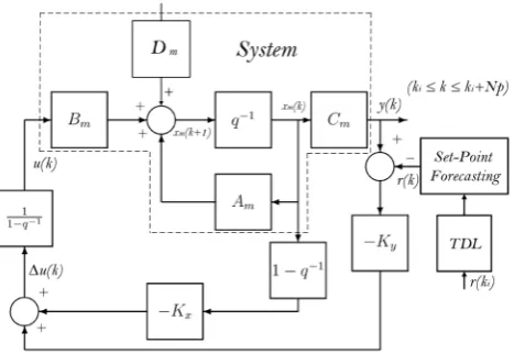
K_y, K_x and K_mpc = [K_xK_y] are coefficient matrices. The discrete-time MPC block diagram with set-point forecasting path is shown in Fig. 4.

4- 2- Stability analysis

MPC has been widely applied as an effective control strategy for many industrial applications, and its stability has also

been under study [32]. There are some studied cases in the

with sufficiently large prediction horizon (or infinite horizon) and stability of MPC with terminal-state penalty in the cost function [30], [33] and [34]. In this paper, the finite receding horizon MPC (often called classic MPC [35]) with a cost function given in (20) where does not have terminal-state constraints and terminal-state penalty is used to achieve desirable performance of the DG main controller. An approach based on the Lyapunov function was given in [35] to establish the stability of the classic MPC where the model of the controlled system is perfect. The perfect model as defined in [35] is the system model without disturbances. The key point is to find a Lyapunov function for the MPC. To analyze stability of the proposed controller, a similar approach as given in [35] is used. Thus, (26) is rewritten as below:

( )

_mpc

( )

u k

K X k

∆

= −



(27)

where

The closed-loop state-space equations of system are given in (28).

( 1)

( )

( ) (

mpc

) ( )

X k



+ =

AX k



+ ∆

B u k

=

A BK

−

X k



(28) The cost function given in (20) can be rewritten as (29) for the system that will be similar to the cost function of a discrete-time linear quadratic regulator (DLQR).

1

1 ( | ) ( | ) 0 ( | ) ( | )

Np Nc

T T

m m

J X k m k QX k m k − u k m k R u k m k

= =

=

∑

 +  + +

∑

∆ + ∆ + (29)

where

   

= _Q

Q~ ₀0 0 .

2 2×

Q and R2×2 are coefficient submatrices that are located on

the main diagonals of Q and R, respectively. The Lyapunov

function V(X~ (k),k)is chosen as below:

1

* * * *

min

1 0

( ( ), ) Np T( | ) ( | ) Nc T( | ) ( | )

m m

V X k k J X k m k QX k m k − u k m k R u k m k

= =

= =∑ + + +∑∆ + ∆ +

   ₍₃₀₎

Superscript * denotes the optimal values. The stability of the classic MPC is established when the Lyapunov function decreases along the state trajectory:

( ( 1), 1) ( ( ), ) 0

V X k + k+ −V X k k < (31)

Using the proved theorem given in [35], the closed-loop system of the classic MPC is stable and (31) is met when

there exists any Δu*_{(k) such that:}

*T_{( 1| )} *_{( 1| )} T_{( | ) ( | )} *T_{( | )} *_{( | ) 0}

X k + k QX k + k −X k k QX k k  + ∆u k k R u k k∆ < (32)

Using (28) and (32), the following condition can be obtained:

1

2 2 2 2 2 2

( ) ( ) 0

0 0 ( )

T T

mpc mpc mpc mpc

T T

mpc B B B

Nc

A BK Q A BK K RK Q

K I Q R − QF

× × ×

− − + − <

=_ _ Φ Φ + Φ

 

 

(33)

Therefore, if Q and Rare selected appropriately such that

(33) is met, the stability of the proposed controller will be guaranteed. For instance, the stability is guaranteed for chosen Q=I₂×₂ andR=I2×2 where Np=Nc=20.

5- Time-domain simulation results

In this section, the proposed control scheme is applied to

a grid-connected DER with a capacity of 10 MVA and its

performance is investigated under various case studies. The detailed switched model of the system is simulated using PSCAD/EMTDC [31]. A collection of different local load types is considered to be connected to the PC through individual circuit breakers as shown in Fig. 2. The local loads include: (a) two three-phase balanced loads, (b) an induction motor, (c) an imbalanced load and (d) a nonlinear load. In

figures and tables, voltages are expressed in kV, currents in

kA, active (reactive) power in MW (MVAr), load torque in

per-unit (p.u.). For the local load collection, four case studies

are examined where the open/close state of breakers and set-points of active and reactive powers are given in tables in specified time intervals. Also the performance of the proposed control scheme under unbalance voltages of main grid is demonstrated in a case study. In these case studies obtained results are compared with those of PI-based scheme proposed in [6] and CMPC (conventional MPC) scheme. In case study 1 to 7, one DG is considered that is connected to the main grid. The last case study is related to connection and parallel operation of three DERs in a grid-connected multi-bus MG shown in Fig. 1. In all case studies the renewable energy resources are replaced with DC voltage sources, thus the dynamics of them are not considered.

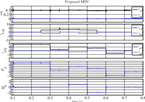
5- 1- Case study 1: Three-phase balanced local load

Two three-phase balanced loads are connected to and disconnected from the PC in a sequence given in Table 2. Simulation results are illustrated in Fig. 5 for the proposed control scheme. As can be observed, active and reactive powers are exchanged very fast and accurately even after each switching instant. Waveforms for two other schemes (PI and CMPC) are the same as those have been shown in Fig. 5 and the schemes have no superiority to each other.

Table 2. Case study 1

time [s] 0-0.1 0.1-0.25 0.25-_0.35 0.35-_0.45 0.45-_0.55 0.55-_0.8

B1_1 O O C C C O

B1_2 O O O C O O

time [s] 0-0.1 0.1-_0.3 0.3-_0.4 0.4-_{0. 5} 0.5-0.6 0.6-0.7 0.7-_0.8

P_g 0 5 1 3 2 -2 0

Q_g 0 0 0 1 -2 0 0

O = open, C = close, P [MW], Q [MVAr]

5- 2- Case study 2: Three-phase imbalanced local load

The three-phase imbalanced load is connected (B3 is closed)

to the PC from t= 0.2 s and is followed by several changes

in set-points of active and reactive powers as given in Table

1. This load (R₃=1 [mΩ] and L₃=3 [µH]) is selected greater

(about 7 times) than that presented in Table 1. Fig. 6 to 8 illustrate the results of three control schemes. A comparison of the results is illustrated in Fig. 9. In Fig.9 (a) to (c) waveforms of the injected currents to the upstream grid are shown. As

can be seen, injected currents when proposed scheme is used are pure sinusoidal balanced currents. The better steady-state performance of the proposed scheme is clearly observed.

When the imbalanced load is connected to the PC at t=0.2

s, P_g and Q_g are distorted by 2ω rad/sec ripple components

for the PI-based control scheme and CMPC due to portion

of imbalanced local load currents i_Labc drawn from main grid.

Such ripples are very little in P_g and Q_g for the proposed

control scheme, and exchanged powers are very smooth (see Fig. 9(d) and (e)). As Fig. 6 to 8 shown, the performance of the PI-based is better than CMPC, but the proposed control scheme demonstrates much desired performance in comparison with two other schemes.

5- 3- Case study 3: Nonlinear and imbalanced local load

The same sequence of events as the case study 2 is considered

for this study where addition to B3, B4 is also closed at t=0.2

s. In this case study, R₄=300 [mΩ] and L₄=10 [µH] are greater

than those in Table 1. Fig. 10, 11 and 12 illustrate the obtained results of three control schemes. Although the three schemes can successfully regulate the powers to their set-points, the steady state performance of the proposed scheme is much better as can be observed in Fig. 13.

5- 4- Case study 4: Induction motor starting

The effectiveness of the proposed scheme is studied for starting an induction motor. The sequence of events is given in 0

0.250.5

vod

q

Proposed MPC

v_od v_oq

-16-8 0 8 16

iLdq

i_Ld i_Lq

-8 -40 4 8

igdq

i_gd i_gq

-20 2 4 6

Pg

0.1 0.2 0.3 0.4 0.5 0.6 0.7 0.8

-20 2

Qg

time (s)

Fig. 5. The results of the proposed control scheme in case study 1.

0 0.250.5

vod

q

Proposed MPC

v_od v_oq

-16-8 0 8 16

iLdq

i

Ld

i

Lq

-8 -40 4 8

igdq

i_gd i_gq

-20 2 4 6

Pg

0.1 0.2 0.3 0.4 0.5 0.6 0.7 0.8

-2 0 2

Qg

time (s)

Fig. 6. The results of the proposed control scheme in case study 2.

0 2 4 6

Pg

CMPC PI Proposed MPC

0.25 0.3 0.35 0.4 0.45 0

2

Qg

time (s)

CMPC PI Proposed MPC

-50 5

igab

c

-50 5

igab

c

-50 5

igab

c

(a)

(b)

(e) (d) (c)

Proposed MPC PI CMPC

Fig. 9. Comparison of the results: (a)-(c): injected currents to upstream grid, (d) and (e): exchanged active and reactive powers when CMPC, PI-based controller and proposed MPC

are used in case study 2.

0 0.250.5

vod

q

CMPC

v_od v_oq

-16-8 0 8 16

iLdq

i_Ld i_Lq

-8 -40 4 8

igdq

i_gd i_gq

-20 2 4 6

Pg

0.1 0.2 0.3 0.4 0.5 0.6 0.7 0.8

-20 2

Qg

time (s)

Fig. 8. The results of the CMPC in case study 2.

0 0.250.5

vodq

PI Controller

v_od v_oq

-16-8 0 8 16

iLdq

i_Ld i_Lq

-8 -40 4 8

igdq

i_gd i_gq

-20 2 4 6

Pg

0.1 0.2 0.3 0.4 0.5 0.6 0.7 0.8

-20 2

Qg

time (s)

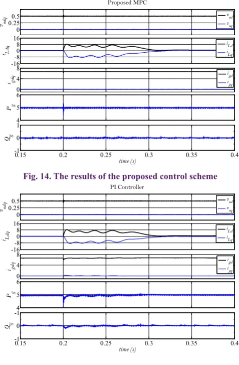
Table 3. Fig. 14, 15 and 16 illustrate the results of three control schemes. As can be seen, the proposed control scheme regulates active and reactive powers accurately. However, the PI-based scheme and CMPC have similar performance for this load condition and cannot properly regulate active and reactive powers. In Fig. 17 the exchanged power for PI-based and the proposed schemes are compared and the superiority of the proposed scheme is evident.

0 0.250.5

vod

q

Proposed MPC

v_od v_oq

-16-8 0 8 16

iLdq

i_Ld i_Lq

-8 -40 4 8

igdq

i_gd i_gq

-20 2 4 6

Pg

0.1 0.2 0.3 0.4 0.5 0.6 0.7 0.8

-20 2

Qg

time (s)

Fig. 10. The results of the proposed control scheme in case study 3.

0 2 4 6

Pg

CMPC PI Proposed MPC

0.25 0.3 0.35 0.4 0.45

0 2

Qg

time (s)

CMPC PI Proposed MPC -50

5

igab

c

-50 5

igab

c

-50 5

igab

c

(a)

(b)

(e) (d) (c)

Proposed MPC PI CMPC

Fig. 13. Comparison of the results: (a)-(c): injected currents to upstream grid, (d) and (e): exchanged active and reactive powers when CMPC, PI-based controller and proposed MPC

are used in case study 3.

0 0.250.5

vod

q

Proposed MPC

v_od v_oq

-16-8 0 8 16

iLdq

i_Ld i_Lq

0 4 8

igdq

i_gd i_gq

4 5 6

Pg

0.15 0.2 0.25 0.3 0.35 0.4

-1 0 1

Qg

time (s)

Fig. 14. The results of the proposed control scheme

0 0.250.5

vod

q

CMPC

v_od v_oq

-16-8 0 8 16

iLdq

i_Ld i_Lq

-8 -40 4 8

igdq

i_gd i_gq

-20 2 4 6

Pg

0.1 0.2 0.3 0.4 0.5 0.6 0.7 0.8

-20 2

Qg

time (s)

Fig. 12. The results of the CMPC in case study 3.

0 0.250.5

vodq

PI Controller

v_od v_oq

-16-8 0 8 16

iLdq

i_Ld i_Lq

-8 -40 4 8

igdq

i_gd i_gq

-20 2 4 6

Pg

0.1 0.2 0.3 0.4 0.5 0.6 0.7 0.8

-2 0 2

Qg

time (s)

Fig. 11. The results of the PI-based control scheme in case study 3.

in case study 4.

0 0.250.5

vodq

PI Controller

v_od v_oq

-16-8 0 8 16

iLdq

i_Ld i_Lq

0 4 8

igdq

i_gd i_gq

4 5 6

Pg

0.15 0.2 0.25 0.3 0.35 0.4

-1 0 -1

Qg

time (s)

Fig. 15. The results of the PI-based control scheme in case study 4.

Table 3. Case study 4

time [s] 0-0.2 0.2-0.4

B2 O C

T_L 0 0.7

Pg 5 5

5- 5- Case study 5:Main grid voltage imbalance

The same sequence of power set-points as the case study 2 is considered for the case study 5. The imbalanced local

load is connected to the PC at t=0.5 s. Main grid voltages are

imbalanced. Therefore v_od and v_oq will oscillate with 2ω-rad/

sec sinusoidal ripple and lead to oscillatory igd*and igq*. Fig. 18,

19 and 20 illustrate the obtained results of the three control schemes. Although the schemes can successfully regulate powers to their set-points, the steady state performance of the proposed scheme is much better, as can be observed in

Fig. 21. As mentioned in section 4, when local load is not

connected yet (up to t=0.5 s), since the sampling time in the

simulation is selected sufficiently small, the profiles of the exchanged active (reactive) power when the proposed control

scheme and CMPC are utilized is similar to each other and are smoother than those of PI-based scheme, but when the

local load is connected (after t=0.5 s), CMPC has no desired

performance in comparison with the proposed and PI-based control schemes(see Fig. 21).

5- 6- Case study 6: Robustness Assessment

In practical applications, system parameters like R, L_f and C_f

are subjected to some uncertainties. To assess the robustness

of the proposed control scheme, -50% mismatch in L_f and C_f

and +100% mismatch in R are supposed and the case study

2 is repeated. As depicted in Fig. 22, the results show stable 0

0.250.5

vodq

CMPC

v_od v_oq

-16-8 0 8 16

iLdq

i_Ld i_Lq

0 4 8

igdq

i_gd i_gq

4 6

Pg

0.15 0.2 0.25 0.3 0.35 0.4

0

Qg

time (s)

Fig. 16. The results of the CMPC in case study 4.

4.5 5.0 5.5

Pg

Proposed MPC PI

0.15 0.2 0.25 0.3 0.35 0.4

-0.5 0 0.5

Qg

time (s)

Proposed MPC PI

Fig. 17. Comparison of the results of the proposed and PI-based schemes in case study 4.

0 0.250.5

vod

q

Proposed MPC

v_od v_oq

-16-8 0 8 16

iLdq

i_Ld i_Lq

-8 -40 4 8

igdq

i_gd i_gq

-20 2 4 6

Pg

0.1 0.2 0.3 0.4 0.5 0.6 0.7 0.8

-20 2

Qg

time (s)

Fig. 18. The results of the proposed control scheme in case study 5.

-2 0 2 4

Pg

CMPC PI Proposed MPC

0.45 0.5 0.55 0.6 0.65

-2 0

Qg

time (s)

CMPC PI Proposed MPC

Fig. 21. Comparison of the results of three schemes in case study 5

0 0.250.5

vod

q

CMPC

v_od v_oq

-16-8 0 8 16

iLdq

i_Ld i_Lq

-8 -40 4 8

igdq

i_gd i_gq

-20 2 4 6

Pg

0.1 0.2 0.3 0.4 0.5 0.6 0.7 0.8

-2 0 2

Qg

time (s)

Fig. 20. The results of the CMPC in case study 5.

0 0.250.5

vodq

PI Controller

v_od v_oq

-16-8 0 8 16

iLdq

i_Ld i_Lq

-8 -40 4 8

igdq

i_gd i_gq

-20 2 4 6

Pg

0.1 0.2 0.3 0.4 0.5 0.6 0.7 0.8

-20 2

Qg

time (s)

performance of the proposed scheme and accurate regulation of exchanged active (reactive) power under the assumed uncertainties.

5- 7- Case study 7: Measurement noises

In this case study, case study 2 is repeated by considering measurement noises. Measurement noises with 20 percent value [36] are supposed for currents in measurement process. Fig. 23 shows the performance of the proposed controller and compares the power profiles with those of case study 2, where no measurement noises exist.

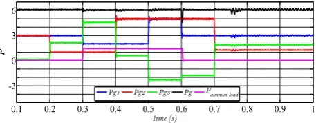
5- 8- Case study 8: Grid-connected operation of a multi-bus MG

In this case study MG described in section 2 is studied. The considered scenario and sequence of events are given in

Table 4. MG must provide 6 MW for the main grid during the

scenario. DGs in addition to powers that deliver to the MG, must provide their local load. Therefore, as aforementioned, active power set-points of DGs which are positive or zero values are dependent on the obtained data from MPPT mechanism (total producible power) and are required active power of their local loads. Those for BT are determined by power balance equation (1) which can be positive or negative or zero. Reactive power set-points are determined based on MG internal consumption and grid operator command. Fig. 24 to Fig. 26 show simulation results for DERs in the MG under given scenario. As can be seen, powers are

exchanged very smoothly under various events. At t=0.75 s,

Table 4. Case study 8

time [s] 0.1-_0.2 0.2-_0.3 0.3-_0.4 0.4-_0.5 0.5-_0.6 0.6-_{0.7 0.75}0.7- 0.75-₁

B3DERs

(local

load) C C C C C O C C

Sc

(common

load) O O C C C O O O

Ssub

(substation

load) O O O O O O O C

P_DER1 3 3 2 2 5 3 3 3

P_DER2 3 1 1 5 5 5 1.25 1.25

P_DER3 0.13 2.13 4.55 0.57 -2.33 -1.81 1.88 1.88

P_demand 6 6 6 6 6 6 6 6

P_{common load} 0 0 1.4 1.4 1.4 0 0 0

P_loss 0.13 0.13 0.15 0.17 0.27 0.2 0.13 0.13 Q_DERs 0.5 0.5 0.8 0.8 0.8 0.5 0.5 0.5 O = open, C = close, P [MW], Q [MVAr]

0.5 1 1.5

Pg

0.3 0.31 0.32 0.33 0.34 0.35 0.36 0.37 0.38 0.39 0.4

-0.5 0 0.5

Qg

time (s)

-2.5 0 2.5

igabc

with noise without noise

with noise without noise

Fig. 23. Zoomed view of the proposed control scheme results in case study 7.

the substation imbalanced load is connected, and due to imbalanced currents which draws from main transformer voltage at low voltage side, is imbalanced. This unbalancing

is propagated to PC voltages of DERs (v_odq oscillate from

t=0.75 s). Delivered powers by DERs under this event are

approximately maintained smooth, but aggregated power injected to the main grid through the main transformer has small amplitude sinusoidal ripple (see Fig. 27). If PI-based control scheme or CMPC is used, aggregated powers delivered will have severe ripples under the given scenario.

6- Conclusions

A control scheme based on MPC is proposed for the main controller of inverter-based DERs to regulate active and reactive powers exchanged between DERs and on-grid system. Active and reactive power control change to current control and the set-points are forecast to improve DER

0 0.250.5

vodq

MPC Controller

v_od v_oq

-16-8 0 8 16

iLdq

i_Ld i_Lq

-8 -40 4 8

igdq

i_gd i_gq

-20 2 4 6

Pg

0.1 0.2 0.3 0.4 0.5 0.6 0.7 0.8

-20 2

Qg

time (s)

Fig. 22. The results of the proposed control scheme in case study 6.

0 0.250.5

vodq

DER1

v_od v_oq

-2 0 2

iLdq

i_Ld i_Lq

-8 -40 4 8

igdq

i_gd i_gq

-20 2 4 6

Pg

0.10 0.2 0.3 0.4 0.5 0.6 0.7 0.8 0.9 1

1 2

Qg

time (s)

performance under various types of local loads and voltage imbalance of the main grid. While imbalanced/nonlinear and induction motor loads as local loads are switching or bus voltages are imbalanced, the regulation is performed properly and smoothly. The control scheme enables an accurate active/

reactive power regulation in connecting the DER to a

multi-bus grid-connected MG in parallel operation with other

DERs. The proposed control scheme presents much better performance in comparison with the PI-based control scheme and CMPC.

References

[1] G. Pepermans, J. Driesen, D. Haeseldonckx, R. Belmans,

W. Dhaeseleer, Distributed generation: Definition, benefits and issues, Energy Policy, 33(6): (2005) 787–98.

[2] T. C. Green, M. Prodanovic, Control of inverter-based

micro-grids, Electr. Power Syst. Res. Distrib. Generation, 77(9) (2007) 1204–13.

[3] J. Rocabert, A. Luna, F. Blaabjerg, P. Rodriguez, Control

of Power Converters in AC Microgrids, IEEE Trans. on Power Electronics, 27(11) (2012) 4734-4749.

[4] F.A. Bhuiyan, A. Yazdani, Energy Storage Technologies

for Grid-Connected and Off-Grid Power System Applications, IEEE Electrical Power and Energy Conference, 2012.

[5] A. Deihimi, B. Keshavarz Zahed, R. Iravani, An

interactive operation management of a micro-grid with multiple distributed generations using multi-objective uniform water cycle algorithm, Energy, 106 (2016) 482-509.

[6] A. Yazdani, R. Iravani, Voltage-Sourced Converters

in Power Systems: modeling, control and applications, IEEE Wiley Press, 2010.

[7] L. Shang, J. Hu, Sliding-mode-based direct power

control of grid-connected wind-turbine-driven doubly fed induction generators under unbalanced grid voltage conditions, IEEE Trans. Energy Conversion, 27(2) (2012) 362–373.

[8] L. Shang, D. Sun, J. Hu, Sliding-mode-based direct

power control of grid-connected voltage-sourced inverters under unbalanced network conditions, IET Power Electron, 4(5) (2011) 570–579.

[9] M.M, Rezaei, J. Soltani, A robust control strategy for

a grid-connected multi-bus microgrid under unbalanced load conditions, Electrical Power and Energy Systems, 71 (2015) 68-76.

[10] M. Mehrasa, E. Pouresmaeil, B. N. Jørgensen, J. P.S. Catalão, A control plan for the stable operation of microgrids during grid-connected and islanded modes, Electric Power Systems Research, 129 (2015) 10-22.

[11] A. H. Syed, M.A. Abido, New enhanced performance robust control design schemefor grid-connected VSI, Control Engineering Practice, 53 (2016) 92-108.

[12] E. Pouresmaeil, O. Gomis-Bellmunt, D. Montesinos-Miracle, J. Bergas-Jané, Multilevel converters control for renewable energy integration to the power grid, Energy, 36 (2011) 950-363.

[13] J. Hu, J. Zhu, D. G. Dorrell, Model predictive control of inverters for both islanded and grid-connected operations in renewable power generations, IET Renewable Power Generation, 8(3) (2013) 240-248.

[14] V. Yaramasu, B. Wu, Model predictive decoupled active and reactive power control for high-power grid-connected four-level diode-clamped inverters, IEEE Trans. Power Electron, 61(7) (2014) 3407–3417.

[15] R. Halvgaard, L. Vandenberghe, N.K. Poulsen, H. Madsen, J.B. Jørgensen, Distributed model predictive control for smart energy systems, IEEE Trans. Smart Grid, 7(3) (2016) 1675-1682.

[16] A.S. Ashtari, A. Khaki Sedigh, Adaptive Simplified Model Predictive Control with Tuning Considerations, Amirkabir International Journal of Science& Research, 46(2) (2014).

0 0.250.5

vod

q

DER2

v_od v_oq

0

iLdq

i

Ld

i

Lq

-8 -40 4 8

igdq

i_gd i_gq

-20 2 4 6

Pg

0.1 0.2 0.3 0.4 0.5 0.6 0.7 0.8 0.9 1

0 1 2

Qg

time (s)

Fig. 25. The results of DER2 for the proposed control scheme in case study 8.

0 0.250.5

vodq

DER3

v_od v_oq

-8 -40 4 8

igdq

i_gd i_gq

-20 2 4 6

Pg

0.1 0.2 0.3 0.4 0.5 0.6 0.7 0.8 0.9 1

0 1 2

Qg

time (s)

Fig. 26. The results of DER3 for the proposed control scheme in case study 8.

0.1 0.2 0.3 0.4 0.5 0.6 0.7 0.8 0.9 1 -3

0 3 6

P

time (s)

Pg1 Pg2 Pg3 Pg P_{common load}

[17] P. Kou, D. Liang, L. Gao, F. Gao, Stochastic coordination of plug-In electric vehicles and wind turbines in microgrid: a model predictive control approach, IEEE Trans. Smart Grid, 7(3) (2016) 1537-1551.

[18] J. Rodriguez, P. Cortes, Predictive Control of Power Converters and Electrical Drives, IEEE Wiley Press, 2012.

[19] L. Tarisciotti, P. Zanchetta, A. Watson, S. Bifaretti, J. C. Clare, Modulated model predictive control for a 7- level cascaded H-bridge back-to-back converter, IEEE Trans. Ind. Electron, 61(2) (2014) 5375-5383.

[20] K. M. Abo-Al-Ez, A. Elaiw, X. Xia, A dual-loop model predictive voltage control/sliding-mode current control for voltage source inverter operation in smart microgrids, Electric Power Components and Systems, 42(3) (2014) 348-360.

[21] P. Cortés, G. Ortiz, J. I. Yuz, J. Rodriguez, S. Vazquez, L. G. Franquelo, Model predictive control of an inverter with output LC filter for UPS applications, IEEE Trans. Ind. Electron, 56(6) (2009) 1875-1883.

[22] K. T. Tan, X. Y. Peng, P. L. So, Y. C. Chu, M. Z. Q. Chen, Centralized Control for Parallel Operation of Distributed Generation Inverters in Microgrids, IEEE Trans. On Smart Grid, 3(4) (2012) 1977-1987.

[23] D. Song, J. Yang, M. Dong, Y. H. Joo, Model predictive control with finite control set for variable-speed wind turbines, Energy, Accepted Manuscript (2017).

[24] M. Hamzeh, H. Karimi, H. Mokhtari, Harmonic and Negative-Sequence Current Control in an Islanded Multi-Bus MV Microgrid, IEEE Trans. On Smart Grid, (2013).

[25] S. K. Chung, A phase tracking system for three phase utility interface inverters, IEEE Transactions on Power

Electronics, 5(3) (2000) 431-438.

[26] A. Medjber, A. Guessoum, H. Belmili, A. Mellit, New neural network and fuzzy logic controllers to monitor maximum power for wind energy conversion system, Energy, 106 (2016) 137-146.

[27] S. Ganjefar, A. Mohammadi, Variable speed wind turbines with maximum power extraction using singular perturbation theory, Energy, 106 (2016) 510-519.

[28] M. E. Basoglu, B. Çakir, A novel voltage-current characteristic based global maximum power point tracking algorithm in photovoltaic systems, Energy, 112 (2016) 153-163.

[29] S. S. Mohammed, D. Devaraj, T.P. I. Ahamed, A novel hybrid Maximum Power Point Tracking Technique using Perturb & Observe algorithm and Learning Automata for solar PV system, Energy, 112 (2016) 1096-1106.

[30] L. Wang, Model Predictive Control System Design and Implementation Using MATLAB, London, 2009.

[31] PSCAD/EMTDC v. 4.5.0.0, Manitoba HVDC Research Centre, Winnipeg, MB, Canada, 2012.

[32] J. Lofberg, Linear Model Predictive Control Stability and Robustness, Sweden, 2001.

[33] L. Grune, J. Pannek, Nonlinear Model Predictive Control: Theory and Algorithems, Springer Press 2017.

[34] J. M. Maciejowski, Predictive Control with Constraints, London, 2000.

[35] W. H. Chen, Stability Analysis of Classic Finite Horizon Model Predictive Control, International Journal of Control, Automation and Systems, 8(2) (2010) 187-197.

[36] N. Suyaroj, N. Watson, Transients State Estimation with Measurement Noise, IEEE Conference, 2015.

Pleasecitethisarticleusing:

A. Saleh, A. Dehimi, Model Predictive Control of Distributed Energy Resources with Predictive Set-Points for Grid-Connected Operation, AUT J. Elec. Eng., 50(2) (2018) 109-120.