L. Grigori, C. Japhet, P. Moireau, Editors
COMPONENT MAPPING AUTOMATION FOR PARAMETRIC COMPONENT
REDUCED BASIS TECHNIQUES (RB-COMPONENT)
∗Rachida Chakir
1, Charles Dapogny
2, Caroline Japhet
3, Yvon Maday
4,
Jean-Baptiste Montavon
5, Olivier Pantz
6and Anthony Patera
7Abstract. The aim of this paper is to develop some techniques for automation of the mappings (between working and reference domains) required by reduced basis methods: the development of geometry mappings is indeed often a substantial impediment to the implementation of reduced basis techniques, especially in the context of the reduced basis element method (RBEM) and the reduced basis component method (RBCM). In the RBCM context, the geometry mappings are applied at the level of components. The methods have been tested on various cases to understand the limits of the approach and try to foresee and overcome the possible failures.
R´esum´e. Le but de cet article est de d´evelopper certaines techniques d’automatisation des transfor-mations (entre domaine de travail et domaine de r´ef´erence) requis par les m´ethodes des bases r´eduites: le calcul de telles applications g´eom´etriques est en effet souvent une entrave importante `a la mise en œuvre de m´ethodes des bases r´eduites, en particulier dans le contexte de la RBEM (Reduced Basis Element Method) et de la RBCM (Reduced Basis Component Method). Dans le cadre des m´ethodes RBCM, les transformation de la g´eom´etrie sont appliqu´ees au niveau des composantes. Les m´ethodes ont ´et´e test´ees sur divers cas pour appr´ehender les limites de l’approche et essayer de pr´evoir et de surmonter les possibles failles.
∗This work was supported by an MIT Ford Professorship and by Akselos, S.A.(Switzerland)
1Universit´e Paris Est, IFSTTAR, 14-20 Bd Newton, Cit´e Descartes Champs sur Marne, 77447 Marne-la-Vall´ee Cedex 2, France, E-mail: [email protected]
2 Laboratoire Jean Kuntzmann, CNRS, Universit´e Grenoble-Alpes, BP 53, 38041 Grenoble Cedex 9, France, E-mail: [email protected]
3 Universit´e Paris 13, Sorbonne Paris Cit´e, LAGA, CNRS UMR 7539, 99 Avenue J-B Cl´ement, 93430 Villetaneuse, France, E-mail: [email protected]
4 Sorbonne Universit´es, UPMC Universit´e Paris 06 and CNRS UMR 7598, Laboratoire Jacques-Louis Lions, F-75005, Paris, France, E-mail: [email protected]; and Institut Universitaire de France; and Division of Applied Mathematics, Brown University, Providence RI, USA
5 Universit´e Paris 13, Sorbonne Paris Cit´e, LAGA, CNRS UMR 7539, 99 Avenue J-B Cl´ement, 93430 Villetaneuse, France, E-mail: [email protected]
6 Universit´e de Nice Sophia-Antipolis, Laboratoire J.A. Dieudonn´e, UMR CNRS 7351, Parc Valrose, 06108 Nice Cedex 02, France, E-mail: [email protected]
7 Department of Mechanical Engineering, Massachusetts Institute of Technology, 77 Massachusetts Avenue, Cambridge, MA 02139, USA, E-mail: [email protected]
c
EDP Sciences, SMAI 2018
−∆φ = 0 in Ωρ, φ = gf on Γf,
φ = 0 on Γρ,
(1)
where the boundary∂Ωρ is composed of two parts: ∂Ωρ= Γf∪Γρ with Γρthe parameter dependent boundary
of the parametrized domain and Γf the fixed boundary (possibly empty) andgf is an appropriate function.
Classical discretization techniques, such as finite element methods, may be too expensive if multiple reso-lutions are required or real-time response is expected. In this perspective, the Reduced Basis (RB) method [1, 16, 18] exploits the parametric structure of the PDE to construct fast and computationally efficient approxi-mations.
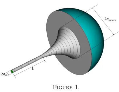
To be even faster the RB method may be combined with Domain Decomposition and leads to component-based RB approaches namely the reduced basis element method (RBEM) [14, 15] and the reduced basis com-ponent method (RBCM) [11, 12, 19]. In these versions of the reduced basis method, the domain of interest Ωρ (where the PDE is set) is decomposed into a series of subdomains with simple shapes called components
Ωρ =∪Kk=1Ck,ρ [5, 10]. Let us consider for example the case of Fig. 1 that represents the spatial domain of a
horn for which the lengthLand the radiia0 andamouthcan vary [13].
Figure 1.
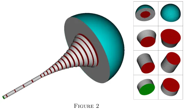
Figure 2
Each of the components featured in there is obtained by deformation of one reference component chosen among a set of few reference components. Each reference component is provided with some basis functions (reduced basis functions) that represent the behavior of the set of all the PDE solutions on such subdomains. The restriction of the solution to (1) to every component is then sought as a linear combination of those basis functions mapped onto the component from the associated reference component.
The objective of this RB-Component project is to rapidly propose the mapping that needs to be used to transfer back and forth all the informations (mesh, reduced basis, geometrical factors) from the reference components to each associated subdomain in Ωρin order to solve the PDE of interest on the global domain Ωρ.
It is not uncommon to use the elasticity equation to lift boundary data into the interior for the purpose of geometry mappings (for example, for ALE fluids calculations) or mesh generation, see [6, 8, 20, 21].
In our approach we propose new strategies to generate these maps using the solutionuuuto a linear elasticity problem. Each new subdomain is obtained by deforming the appropriate reference component through a map
T : ¯xxx7→xxx¯+uuu(¯xxx) that only has to send the boundary of the reference component onto the boundary of the subdomain.
The different methods that have been tested differ from the way the displacementsuuuare imposed on the com-ponent boundary. The first technique that we have investigated, consists in simply imposing classical Dirichlet boundaries conditions, but it requires an explicit parametric definition of the boundary component, which is not always possible. The second approach that we have studied, consists in a penalization method which only requires an implicit caracterization of the boundary; though this description of the boundary is less precise it appears sufficient for our purpose.
In what follows we shall focus on a single component, in the sense that we do not perform any domain decomposition. There is thus only one reference component and the corresponding deformed component. In Sec. 1, we tested these different approaches to build an automatized mapping in order to solve Laplace problems as (1) over different kinds of geometry. Then, in Sec. 2 we present the mapping used in a reduced basis method context.
1.
Computation of the displacement field for the mapping and resolution of
the Laplace equation on the deformed domain
Letρbe a set of geometrical factors used to parameterize the geometry of the unique componentC1,ρ≡Ωρ
whereuuu(¯xxx) = (u1(¯xxx), u2(¯xxx)) is the displacement. As said above, we choose that the displacement is the solution of a linear elasticity problem over the reference domain Ωref:
Finduuu∈V such that
Z
Ωref
2µ eee(uuu) :eee(vvv) +λdiv (uuu) div (vvv)dxx¯x= 0, ∀vvv∈(H01(Ωref))2, (3)
whereV is a space that is in some sense defined as (the precise definition being given hereafter)
V ' {vvv= (v1, v2)∈(H1(Ωref))2; vvv= 000 on Γf; ¯xxx+vvv(¯xxx)∈Γρ, ∀xx¯x∈Γref},
(λ, µ) = ((1+νEν)(1−2ν),2(1+Eν)) are the Lam´e coefficients, withE the Young’s modulus andν the Poisson’s ratio, andeeeis the linearized strain tensor given by
eee11(uuu) = ∂x¯1u1, eee22(uuu) = ∂x¯2u2,
eee12(uuu) = eee21(uuu) = 21(∂x¯2u1+∂x¯1u2),
(4)
with the notationeee(uuu) :eee(vvv) :=X
i,j
eeei,j(uuu)eeei,j(vvv).
It is classical, and will be instrumental for our approach, to remind that problem (3) is linked to the problem of minimizing the energy
J(www) = 1 2
Z
Ωref
λ(div (www))2+ 2µX i,j
eeei,j(www)2)dxx¯x. (5)
and the first choice of spaceV, in line with this minimization process, is called here an explicit version (called also “pointwise”) : assuming that s7→xx¯x(s) (resp. s7→xxx(s)) is a one-to-one parametrization of Γref (resp. of Γρ):
V =Vexplicit:={vvv= (v1, v2)∈(H1(Ωref))2; vvv= 000 on Γf; vvv(¯xxx(s)) =xxx(s)−x¯xx(s),∀s}.
At this level it is interesting to recall that there are two ways to impose Dirichlet boundary conditions: the strong one where the discrete solution belongs toV and the weak one where the boundary condition is satisfied through a penalization formulation. In what follows we will first test these two ways and then focus on the weak one that appears much more simple to implement. In addition the weak formulation only requires an implicit caracterization of the boundary which is generally much more simple than having a parametrization (especially in higher dimension that will be dealt in a future paper Ωρ ∈ R3). This leads us to introduce an
implicit version (called also “slippery”) of the space V : assuming that Γρ is defined as the set of pointsxxxin R2 such thatFρ(xxx) = 0:
V =Vimplicit:={vvv= (v1, v2)∈(H1(Ωref))2; vvv= 000 on Γf; Fρ(¯xxx+vvv(¯xxx)) = 0, ∀xx¯x∈Γref}.
Let us now proceed to the use of the map from the reference domain: a simple change of variables leads to
Z
Ωρ
∇φ· ∇v dxxx= 0 =
Z
Ωref
with
K=J−1J−t|J|, (6)
whereJ is the Jacobian matrix ofTTT:
J =
∂x¯1x1 ∂x¯2x1 ∂x¯1x2 ∂x¯2x2
=
∂x¯1(T1(¯xxx)) ∂x¯2(T1(¯xxx)) ∂x¯1(T2(¯xxx)) ∂x¯2(T2(¯xxx))
andJ is det(J), more precisely, this reads
K= 1
|J|
(∂x¯2(T2(¯xxx)))
2+∂
¯
x2(T1(¯xxx))
2 −(∂
¯
x1(T2(¯xxx))∂x¯2(T2(¯xxx)) +∂x¯2(T1(¯xxx))∂x¯1(T1(¯xxx)))
−(∂x¯1(T2(¯xxx))∂x¯2(T2(¯xxx)) +∂¯x2(T1(¯xxx))∂¯x1(T1(¯xxx))) (∂x¯1(T2(¯xxx))) 2+ (∂
¯
x1(T1(¯xxx))) 2
(7) withJ =∂x¯1(T1(¯xxx))∂x¯2(T2(¯xxx))−∂¯x2(T1(¯xxx))∂¯x1(T2(¯xxx)).
One convenient way to verify that the mapping as defined above is correct, with respect to our aim which is to simulate partial differential equation on Ωρ, is to consider the Laplace problem (1) over Ωρ that we state
here under a weak formulation: Findφ∈W :={z∈H1(Ω
ρ); z=gf on Γf; z= 0 on Γρ}such that, ∀v∈H01(Ωρ):
Z
Ωρ
∇φ· ∇v dxxx= 0 =
Z
Ωρ
∂x1φ ∂x1v+∂x2φ ∂x2v dxxx. (8)
In what follows we tested different approaches to compute the displacements uuu which will be used in the mappingTTTfor several test cases. All the simulations have been done usingP1finite element withinFreefem++[7]. Several examples are presented to compare different solution algorithms but also different treatments ofFρ(e.g.,
explicit versus implicit). More precisely, we first present in Sec. 1.1.1, a circular hole with pointwise Dirichlet strong boundary conditions, which are the natural way to impose the displacement on the boundary Γρ. As
it is difficult to use strong Dirichlet conditions for the general case, and we propose instead to use a penalized approach: we provide in Sec. 1.1.2 a comparison with penalized Dirichlet conditions. Then we consider a uniform shear square (with linearFρ) with strong (in Sec. 1.1.3), and penalized (in Sec. 1.2.1) Dirichlet conditions. The
conclusion is that we do not loose much when using a penalized formulation. Thus we use a penalized version to treat increasingly more complex deformations: a non-uniform shear square (with nonlinearFρ) in Sec. 1.2.2,
then a bell (with nonlinear and large amplitudeFρ) in Sec. 1.2.3, and finally a crescent moon with a cusp, in
Sec. 1.2.4.
1.1.
Computation of the displacement using Dirichlet boundary conditions
1.1.1. Example 1: square with a circular hole and strong Dirichlet boundary conditions
c
¯
a
Γref
Γa u
u u
Γf Γf
c a
Γa
Figure 3. Left: reference domain Ωref; Right: generic parameter dependent domain Ωρ.
In this example the set of parameter ρ is made up of the radius a. In the generic parameter dependent domain Ωρ, the boundary Γa represents the parameter dependent boundary Γρ. To compute a displacementuuu
that describes the mapping from the reference domain Ωref to the generic domain Ωρ, we solved a linear
elas-ticity problem with homogenous Dirichlet boundary condition on the fixed boundary Γf, and non homogenous
Dirichlet boundary condition
u1= (
a
¯
a−1)¯x1, u2= ( a
¯
a−1)¯x2,
on Γref – which represents the boundary of the reference domain that will be deformed in order to get the generic boundary Γρ = Γa :
u u
u(¯xxx) = (a¯a −1)¯xxx for ¯xxx∈Γref. (9)
In what follows we choose to set the Young modulus toE= 1 and the Poisson ratio toν =14.
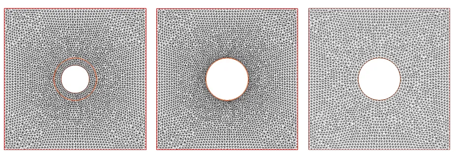
Figure 4. reference meshTref (left), deformed mesh Tmap (middle) and true mesh Th of the generic domain (right).
In Fig. 4 we represented the mesh Tref – a regular triangulation with 200 vertices on Γa and 50 vertices on
Γref – associated to the reference domain (for ¯a= 0.2) (left), and meshes associated to the generic domain (for
domain Ωρ (right) built independently but similarly asTref. We observe that the deformed mesh fits well with the objective (larger red circle represented on left and middle meshes of Fig. 4) and, at least from the eye point of view, appears rather regular and quite similar to the meshTh with 200 vertices on Γf and 50 vertices on Γa.
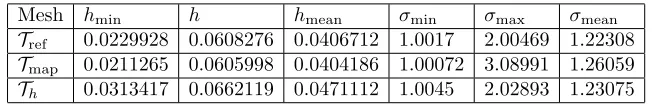
In order to better quantify the quality of a mesh, we produce in Table 1 below classical quantities associated to the mesh. As usual, we denote by h, hmin, hmean the maximum, minimum and average mesh size of Th, respectively. We also introduce ˜σT = hρT
T, where ρT is the diameter of the incircle of a triangle T ⊂ Th, and
for referenceσT = ˜σTσ
ˆ
T
, where ˆT is an equilateral triangle. Then σ, σmin, σmeandenote the maximum, minimum and average ofσT forT ⊂ Th, respectively. These results highlight the regularity of the mesh obtained by our
transformation.
Mesh hmin h hmean σmin σmax σmean
Tref 0.0229928 0.0608276 0.0406712 1.0017 2.00469 1.22308
Tmap 0.0211265 0.0605998 0.0404186 1.00072 3.08991 1.26059
Th 0.0313417 0.0662119 0.0471112 1.0045 2.02893 1.23075
Table 1. Example 1: classical quantities associated to the meshesTref,Tmap andTh
We denote byX0
h theP1 finite element approximation ofH01(Ωρ) associated to the mesh Th and byXh the P1 finite element approximation of X ={z ∈H1(Ωρ); z =f on Γf; z= 0 on Γρ} associated to the meshTh.
Letφh∈Xh be the solution of the true discrete approximation of (8)
Z
Th
∇φh· ∇ψhdxxx= 0 ∀ψh∈Xh0. (10)
We denote byX0
map theP1 finite element approximation ofH01(Ωρ) associated to the mesh Tmap and Xmap theP1finite element approximation ofX associated to the meshTmap. Let φmap ∈Xmap be the solution of the following discrete approximation of (8)
Z
Tref
K∇xx¯x(φmap◦TTT)· ∇xxx¯(v◦TTT)dxxx¯= 0, ∀v∈Xmap0 , (11)
whereK is the mapping matrix defined by (6).
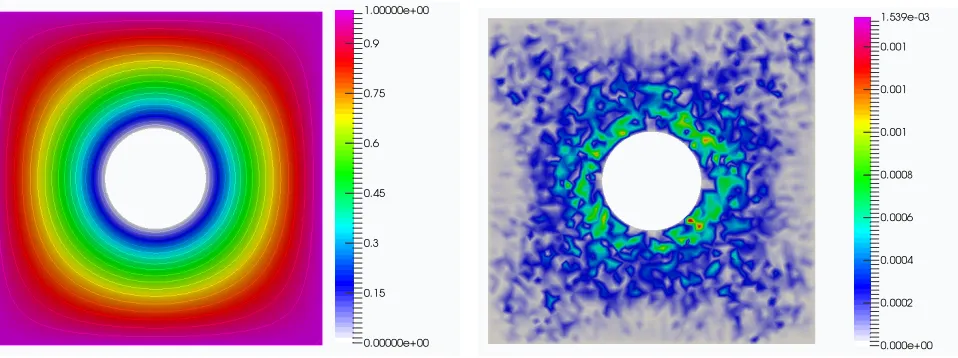
In order to validate this mapping approach to solve our Laplace problem (8) withgf = 1 and Γρ= Γa. We
have computed a true discrete approximation on the meshThand approximation using the mapping approach with ¯a= 0.2 anda= 0.3.
In Fig. 5 we show the solutionφmap (left) and the relative error measured in theL∞-norm betweenφh and Ihφmap, whereIh is the interpolation operator fromXmap intoXh.
This error is on the order ofh2, wherehis the maximum mesh size ofT
h(see Table 1), as might be expected
Figure 5. Left: solutionφmap; Right: relative error betweenφh andIhφmap.
1.1.2. Example 2: square with a circular hole and penalized Dirichlet boundary conditions
In this section we replace, in the linear elasticity problem, the non-homogeneous Dirichlet boundary condition on Γρ by
uuu−(¯a−a)nnn= 0.
This boundary condition is imposed in a weak form, using a (quadratic) penalty method: we replace the constrained minimization problem
inf
w
ww∈V0;www−(¯a−a)nnn=0
J(www), (12)
by the unconstrained problem
inf
w ww∈V0
J(www) +
1
G(www)
, (13)
with
V0={vvv∈H1(Ωref))2; v1=v2= 0 on Γf} (14)
and
G(www) =
1 2
Z
Γref
|www−(¯a−a)nnn|2dΓ.
Letuuube the solution of minimisation problem (12) anduuu the solution of minimisation problem (13), we have
kuuu−uuuk −→ →00.
Besides, finding a solution to the minimisation problem (13) is equivalent to finding a solution to the following variational problem: Finduuu∈V0, such that∀vvv∈V0,
h∇J(uuu), vvviV
0,V00+
1
h∇G(uuu), vvviV0,V00 = 0,
which can be rewritten as follows : Finduuu∈V0, such that ∀vvv∈V0,
Z
Ωref
2µ eee(uuu) :eee(vvv) +λdiv (uuu) div (vvv)dxx¯x+1
Z
Γref
Figure 6. Left: reference meshTref; Right: deformed meshTmap.
In Fig. 6 we represented the meshTref associated to the reference domain (for ¯a= 0.2) (left), and the mesh associated to the generic domain (fora= 0.3) : the deformation of Tref due to displacementuuu (right), which is very similar to the mesh obtained in the previous approach where we imposed non-homogenous Dirichlet boundary conditions on Γρ= Γa. As done in the previous example, in order to better quantify the quality of a
mesh, we produce in Table 2 quantities associated to the meshTmap obtained by our mapping (see Sec. 1.1.1). The quantities associated toTref andThare already given in Table 1. Again, the results highlight the regularity
of Tmap. Moreover, we observe that the results of Table 1 and Table 2 are almost the same, and thus using penalized conditions appears to be a good alternative to using strong boundary conditions.
Mesh hmin h hmean σmin σmax σmean
Tmap 0.0211276 0.0605997 0.0404187 1.0007 3.09102 1.26065
Table 2. Example 2: classical quantities associated to the meshTmap
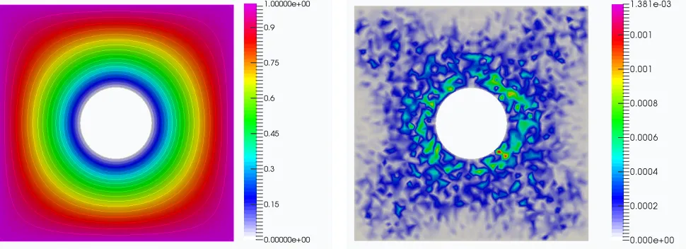
Figure 7. Left: solutionφmap; Right: relative error betweenφh andIhφmap.
¯ Γ3ref
Ωref Γf
¯ Γ1ref
¯ Γ2
ref
(0,0) (1,0)
(0,1) (1,1)
(0,0) (0,1)
(α,0)
(α+β,1)
Γ1ρ
Γ2
ρ
Γ3
ρ
Γf Ωρ
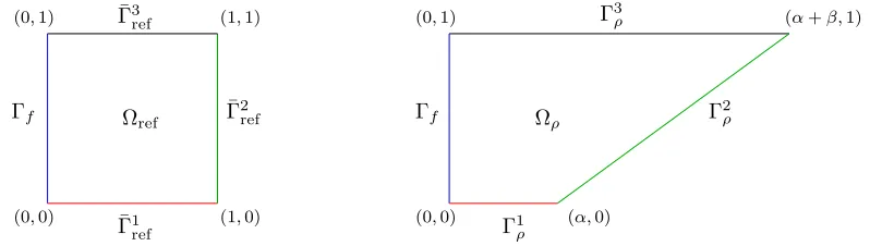
Figure 8. Left: reference domain Ωref; Right: generic domain Ωρ.
The set of varying parametersρis made of the coefficientαandβ. In the generic domain Ωρ, the parameter
dependent boundary Γρ is made of the union of Γiρ, 1≤i≤3 and respectively Γref is made of the union of ¯Γiref, 1≤i≤3.
In order to compute the displacement that describe the mapping from the reference domain Ωref to the generic domain Ωρ we associate the following Dirichlet boundary conditions to the linear elasticity problem
u1 = (α−1)¯x1 on Γ1ρ u1 = (α+ ¯x2β−1)¯x1 on Γ2ρ, u1 = (α+β−1)¯x1 on Γ3ρ
u1 = 0 on Γf,
u2 = 0 on∂Ωρ.
In Fig. 9 we represented the meshTref – a regular triangulation with 50 vertices on Γf and each Γiρ, 1≤i≤3
– associated to the reference domain (left) and the deformed mesh Tmap for α = 2 and β = 1 (right). As previously, we observe that the mapped mesh fits well with the objective (in green).
Figure 9. Left: reference meshTref; Right: deformed meshTmap.
Figure 10. meshThof generic domain Ωρ withα= 2 andβ= 1
Figure 11. Left: solutionφmap; Right: relative error betweenφh andIhφmap.
We consider now the Laplace problem (8) withgf = (1−x2)x2. In Fig. 11 we show the solutionφmap (left) and the relative error measured in theL∞-norm betweenφhandIhφmap, whereIhis the interpolation operator
fromXmap intoXh. This error is approximatelyO(h2) wherehis the mesh size of Th. As expected, the error
is on the order ofh2 as in the previous examples.
1.2.
Computation of the displacement using a penalty method
The technique that we have investigated in section 1.1 consisted in simply imposing Dirichlet boundary conditions in order to control the displacementsuuuon the component boundary such that the deformation of the reference domain Ωref matches with the generic domain Ωρ. However, this approach requires an explicit
parametric definition of the boundary component, which is not always possible. The second approach, that we now present, only requires an implicit caracterization of the boundary Γρ. This is done by the use of a
functionalFρ defined such that
Fρ(xxx) = 0, on Γρ.
The idea is to compute a displacementuuusuch thatFρ(¯xxx+uuu(¯xxx)) = 0 on the boundary Γref, which leads to the following constrained minimization problem
inf
w w w∈V0,
Fρ(¯xxx+www)=0 on Γref
J(www), (16)
in which J(www) and V0 are respectively given by (5) and (14). Nevertheless, we decided to weakly impose the constraintFρ(¯xxx+uuu(¯xxx)) = 0 using a penalty approach, which leads to the following unconstrained problem
inf
w w w∈V0
J(www) +
1
Z
Γref
(Fρ(¯xxx+www))2dΓ
we propose different approaches to solve the problem, using a fixed-point method or a steepest descent method.
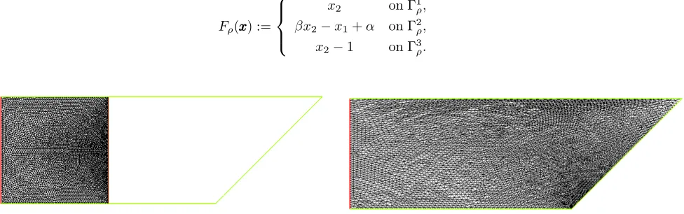
1.2.1. Example 4: deformed (uniform shear) square
In this example we consider the deformation of the unit square [0,1]×[0,1] as in Sec. 1.1.3 ( see Fig. 8). The set of varying parametersρis the same as in Sec. 1.1.3. The reference domain and the associated meshTref, the generic domain and associated mesh Th are also the same as in Sec. 1.1.3. The functionalFρ used to describe
the boundary Γρis defined by:
Fρ(xxx) :=
x2 on Γ1ρ, βx2−x1+α on Γ2ρ, x2−1 on Γ3ρ.
Figure 12. Left: reference meshTref; Right: deformed meshTmap.
In Fig. 12 we represented the reference mesh (left)Tref and the deformed meshTmap with α= 2 andβ= 1 (right). As previously, we observe that the deformed mesh fits well with the objective in green.
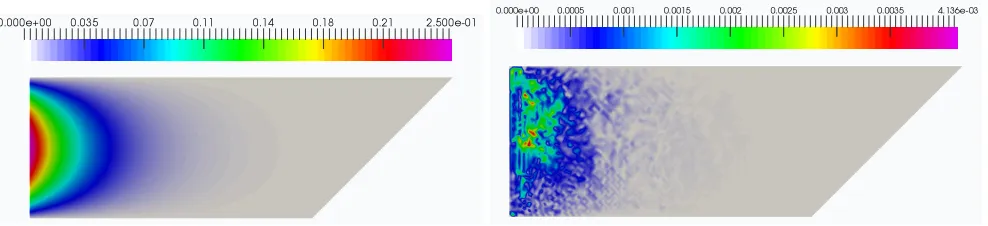
We consider the same Laplace problem as in the example 1.1.3. In Fig. 13 we represented the solution of the Laplace problemφmap (left) and the relative error measured in theL∞-norm betweenφhandIhφmap, whereIh
is the interpolation operator fromXmap intoXh. As expected, this error is on the order ofh2.
1.2.2. Example 5: deformed (non-uniform shear) square
In this second example we still consider the deformation of the unit square [0,1]×[0,1]. The reference domain and the associated meshTref are the same as in Sec. 1.2.1. Besides, the functionalFρ(.) on the boundaries Γ1ρ
and Γ3
ρ is defined similarly as in Sec. 1.2.1. However, now on the boundary Γ2ρ the functional is nonlinear (see
Fig. 14) and defined by:
Fρ(xxx)|Γ2
ρ :=βx2−(x1−α)−β `sin
2πx1−α β
,
In addition to the coefficientsαandβ, the amplitude `will also belong to the set of varying parametersρ.
¯ Γ3 ref Ωref Γf ¯ Γ1 ref ¯ Γ2 ref
(0,0) (1,0)
(0,1) (1,1)
(0,0) (0,1)
(α,0)
(α+β,1)
Γ1 ρ Γ2 ρ Γ3 ρ
Γf Ωρ
Figure 14. Left: reference domain Ωref; Right: generic domain Ωρ.
Because of the nonlinearity ofFρ, we use a Picard fixed-point algorithm to solve problem (18) that can be
rewritten under the form
Aref(uuu, vvv) + ˜f(uu, vu vv) = 0, ∀vvv∈V0,
or equivalently, defining the solution operatorA byAref(Aggg, vvv) =−(ggg, vvv), ∀vvv∈V0 for a givenggg,
u u
u=F(uuu),
withF(uuu) :=A−1F˜(uuu), and ( ˜F(uuu), vvv) = ˜f(uuu, vvv), ∀vvv∈V 0.
Starting from an initial guessuuu0, we solved iteratively the following problem forn= 1,· · ·, n max. Finduuun ∈V
0, such that
u
uun=F(uuun−1),
that is, finduuun∈V
0, such that∀vvv∈V0,
Z
Ωref
2µ eee(uuun) :eee(vvv) +λdiv (uuun) div (vvv)dxxx¯+1
Z
Γref
2Fρ(¯xxx+uuun−1)(∇Fρ(¯xxx+uuun−1), vvv)dΓ = 0, ∀vvv∈V0.
In Fig. 15 we show the reference meshTref (left), and the deformed meshTmapforα= 1,β= 0.7, and`= 0.1 (right). We observe that the deformed mesh fits well with the objective in green.
Tmap 0.00961286 0.0642076 0.0227618 1.00129 3.52419 1.31929
Th 0.00828206 0.0338312 0.0192272 1.00132 2.12118 1.21547
Table 3. Example 1: classical quantities associated to the meshesTref,Tmap andTh
In this example, we consider a Laplace problem (1) wheregf is set togf(xxx) =x2(1−x2) on Γf. In Fig. 16 we
show the solution of the Laplace problemφmap (left) and the relative error measured in theL∞-norm between
φh andIhφmap. As previously, this error is on the order ofh2(see Table 3), as in the previous examples.
Figure 16. Left: solutionφmap; Right: relative error betweenφh andIhφmap.
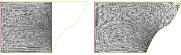
1.2.3. Example 6: deformed square into a bell
In this third example we still consider the deformation of the unit square [0,1]×[0,1]. The reference domain and the associated mesh Tref are the same as in Sec. 1.2.2. The functional Fρ on the boundaries Γ1ρ and Γ3rho
is also defined similarly as in Sec. 1.2.2. However, now on the boundary Γ2
ρ the functionalFρ is defined by:
Fρ(xxx)|Γ2
ρ :=x2−
1 1 +αcos(2πx1)
,
where the coefficientαrepresents the set of varying parametersρ(see Fig. 17).
¯ Γ2
ref
Ωref ¯
Γ3 ref
Γf
¯ Γ1
ref
(0,0) (1,0)
(0,1) (1,1)
(0,0) (0, α)
(1,0) (1, α)
Γf
Γ1
ρ
Γ2
ρ
Γ3
ρ
Ωρ
To treat the nonlinearity of Fρ, we choose to use a steepest-descent method with step size ζ > 0 to solve
problem (18). Starting from an initial guessuuu0, we iteratively compute forn= 0,1,· · · , n max:
u u
un+1=uuun+ζdddn,
wheredddn is the solution to the problem: Finddddn∈V
0, such that∀vvv∈V0,
(dddn, vvv)elas=−(uuun, vvv)elas−
2
Z
Γref
Fρ(¯xxx+uuun)(∇Fρ(¯xxx+uuun), vvv)dΓ,
with (www, vvv)elas:=
Z
Ωref
2µeee(www) :eee(vvv) +λdiv (www)div (vvv)dxxx.¯
Such approach may lead to inverted triangles during the process, thus we propose the following alternatives for the term (dddn, vvv)
elaswhich improve the method:
(dddn, vvv)elas,F :=
Z
Ωref
1
φ(F(xxx+dddn)2) 2µeee(ddd
n) :eee(vvv) +λdiv (dddn)div (vvv) dxxx¯
(dddn, vvv)elas,κ:=
Z
Ωref
1
φ(κ1γ)
2µeee(dddn) :eee(vvv) +λdiv (dddn)div (vvv)
dx¯xx, withγ= 7,
whereφ(t) = 1−e−t, andκis the aspect ratio of triangles, defined byκ= rcirc
2∗rin, wherercircis the radius of the
circumscribed circle, andrin is the radius of the incircle of the triangle.
This idea of changing the inner product whereby a gradient is identified for J(www) is quite classical in the study of gradient flows; it amounts to an efficient preconditioning of the minimization problem (16); see e.g. [4] about this point.
Figure 18. Left: reference meshTref; Middle: deformed meshTmap using (., .)elas,F; Right:
deformed meshTmap using (., .)elas,κ.
In Fig. 18 we represented the reference meshTref (left), and the deformed meshes forα= 0.3, using (., .)elas,F
(middle) and (., .)elas,κ (right). We observe that the mapped mesh fits well with the objective for both cases
the union of Γρ and Γρ, and respectively Γref is made of the union of Γref and Γref.
¯ Γ2
ref ¯
Γ1ref Γf
Ωref Γf
Γf
Γf
(0,0) (1,0)
(0,1) (1,1)
(0,0) (0,1)
(1,0) (1,1)
Γf
Γf
Γf
Γf
Ωρ
Γ2 ρ
Γ1ρ
Figure 19. Left: reference domain Ωref; Right: generic domain Ωρ.
The functional that describes the boundary Γρ is nonlinear and as follows:
Fρ(xxx)|Γ1
ρ := (x1−c)
2
+ (x2−0.5)2−r21,
Fρ(xxx)|Γ2
ρ := (x1−0.5)
2
+ (x2−0.5)2−r22.
To treat the nonlinearity ofFρin (18) we choose to use one of previous steepest descent algorithm with (., .)elas,κ.
The reference mesh Tref is a regular triangulation with 30 vertices on Γf, 20 vertices on Γ1ref and 40 on Γ 2 ref associated to the reference domain for ¯c= 0.4, ¯r1=
√
0.22+ 0.12≈0.22 and ¯r
2= 0.2 . In Fig. 20 we represented the reference mesh (left), and the deformed mesh forc= 0.3,r1= 0.35 andr2= 0.27 (right). We observe that the mapped mesh fits well with the objective.
2.
Recap. on the Reduced Basis Method
In this section we present the mapping used in a reduced basis method context. The implementation is then decomposed in the following independent steps.
2.1.
First step: construction of the manifold of deformations
Following one of the methods presented above, we are able to solve an elasticity problem, the solution of which is a displacement that enables to go from Ωref onto the domain of interest Ωρ and that maps the points
of each part Γm
ref of the boundary of Ωrefinto (actually onto) the associated part Γmρ of Ωρ.
We compute such elasticity solutions for a large numberN of values of ρhopefully representing well the set of all problems we shall be faced to (in our caseN was set to 100). The displacements are denoted asUUU(ρ), these are defined over Ωref, the mapping from Ωrefonto Ωρ isId+UUU(ρ).
Note that the restriction uuum(ρ) = UUU(ρ) |Γm
ref of UUU(ρ) on Γ
m
ref can be considered as a Dirichlet boundary condition for an elasticity problem that maps Ωref onto the domain of interest Ωρ. In opposition to what
generally happens for those Dirichlet boundary conditions, they are not imposed a priori but are obtained a posteriori, after the problem has been solved.
It is expected, verified in our applications — and it would be good to prove it — that the set of all{uuum(ρ)},
when ρ varies is a manifold with a small Kolmogorov n-width, which is the requirement for next building a sensible reduced basis approach (see e.g. [9, 17]).
2.2.
Second step: extraction of a reduced basis for fast approximation of the deformations
for general parameters
We extract with a POD or a greedy procedure (see e.g. [9, 17]) from this manifold {uuum(ρ)} whenρvaries, a
(small) set of parameters ρ1, ρ2, . . . , ρn, . . . such that, for any givenε >0, there existsn=n(ε) such that, for
anyρ, there exists componentsα1(ρ), α2(ρ), . . . , αn(ρ) such that
kuuum(ρ)− n
X
i=1
αi(ρ)uuum(ρi)kL∞(∂Ω
ref)≤ε (19)
By linearity of the elasticity problem, the solution UUU(ρ) to the elasticity problem over Ωref, with Dirichlet
boundary conditionsuuum(ρ) is thus close to n
X
i=1
αi(ρ)UUU(ρi) with an error over Ωrefthat is bounded byCεwhere
C is some stability constant.
Actually, the coefficientsαi(ρ) can be found by many ways from the knowledge of theN solutionsuuum(ρ) that
were computed, but it is also possible to get them for parameters that do not belong to the set of parameters that have been chosen in subsection 2.1. If these chosen values indeed represent well the set of all problems we shall be faced to, then we can propose to define, for any ρthe {αi(ρ)}i=1,...,n by least square applied to the
implicit caracterizationFρ(.) = 0 defining the boundary of Ωρ. This means that
{αi(ρ)}i=1,...,n= arg min {βi}i=1,...,n
Fρ
Xn
i=1
βiuuum(ρi)
L2(∂Ωref) (20)
Having found these values {αi(ρ)}i=1,...,n, an approximation of the elasticity problem that maps Ωref over Ωρ is thus also given byP
n
i=1αi(ρ)UUU(ρi).
The way we solve (19) and (20) is as follows : for (19), an EIM Greedy approach is used to identify theuuuand hence theUUU. For (20), we used a standard matlab nonlinear least-squares solver (’lsqnonlin’). Note that (20) produces the optimal coefficients, and is thus not a POD approach that targets to find the optimalum(ρ
i=1
i i
and
J(ρ) = det
" n
X
i=1
αi(ρ)J(ρi)
#
(22)
which is quadratic in theαi’s.
2.4.
Fourth step: computation of the inverse of the Jacobian determinant
Looking back to (8) we have to evaluate rapidly the contributions in the 2×2 matrix
J−1J−t|J|
that appear in K (see (7)) as a quadratic expression in the displacement — and thus that can be, like the determinant above, be written in terms of a quadratic expression in theαi’s — divided byJ.
Due to this, the complexity in the αis too large and, in order to express K rapidly, we refer to a further
set of approximation. The matrix K:=K(ρ) =
K1,1 K1,2
K2,1 K2,2
:=
K1,1(ρ) K1,2(ρ)
K2,1(ρ) K2,2(ρ)
, and each Kp,q(ρ)
can thus be expressed in terms of a linear combination of Kp,q( ˜ρk), for well chosen parameter values ˜ρk, k = 1, . . . , NK not necessarily coinciding with the set ρi used in the definition of the displacement reduced
basis.
Our purpose is thus to expressK(ρ) as a linear combination ofK( ˜ρk)
K(ρ) =
NK
X
k=1
βkK(ρk) (23)
and this is done through the Empirical interpolation method (EIM) [2] since, thanks to the approximation
U U U(ρ)'
n
X
i=1
αi(ρ)UUU(ρi), we can evaluate easily the gradient ofUUU and then the value atNK appropriate points
x x
xk. These points can and are chosen in such a way that the prescription of the equality of (23) atNK points
leads to a unique definition of the coefficients βk. Note there are two options to approximateK(ρ); we can
develop an EIM approximation for each component of K(ρ), or we can treat the entire matrix with a single EIM approximation. In this article we considered the first option. Note that, for a 2×2 matrix, there is not much difference between the two options. Rather for a larger matrix, the first one is the only that is viable, see [3] for implementation.
2.5.
Numerical results
2.5.1. Square with a circular hole
Figure 21. Solution of Laplace problem
During Online Stage Time to map surface = 0.041
Time to solve RB system =9.3e-04 Time to solve FE system =0.18
Max diff due to EIM = 0.037 Max diff due to RB = 0.002
Table 4. Computational times and error
The Table 4 summarize the computational times and error of the reduced basis method. Here the errors are absolute. However, the solutions are O(1) so relative and absolute are quite similar.
2.5.2. Case of a bell
We consider a 2D test case of a bell. The geometrical parameter isα(see Fig. 17). In Fig. 22 we represented the solution of the Laplace problem (1) by coupling the mapping method to the reduced basis method.
0 0.1 0.2 0.3 0.4 0.5 0.6 0.7 0.8 0.9 1 −0.2
0 0.2 0.4 0.6 0.8 1 1.2
1.4 RB solution, full field
0 0.2
0.4 0.6
0.8 1
−0.5 0 0.5 1 1.5
0 0.2 0.4 0.6 0.8 1
RB solution, full field
In Table 5, the computational times and error of the reduced basis method are shown. Here the errors are absolute. However, the solutions are O(1) so relative and absolute are quite similar.
Acknowledgments
This work is the result of a fruitful collaboration that took place during the CEMRACS 2016. We warmly thank the organizers of the 2016 edition of the CEMRACS and the CIRM for its welcome during the CEMRACS. We thank Dr Phuong Huynh and Loi Nguyen for their assistance with software related to Fig. 1 and Fig. 2.
References
[1] B.O. Almroth, P. Stern, and F.A. Brogan. Automatic choice of global shape functions in structural analysis. AIAA J, 1978. [2] M. Barrault, Y. Maday, N.C. Nguyen, and A.T. Patera, An ’Empirical Interpolation’ Method: Application to Efficient
Reduced-Basis Discretization of Partial Differential Equations. CR Acad Sci Paris Series I 339:667–672, 2004.
[3] D. Bonomi, A. Manzoni, and A. Quarteroni, A matrix DEIM technique for model reduction of nonlinear parametrized problems in cardiac mechanics, Computer Methods in Applied Mechanics and Engineering, 324 (2017), Elsevier, pp. 300–326.
[4] M. Burger,A framework for the construction of level-set methods for shape optimization and reconstruction, Interfaces and Free Boundaries, 5 (2003) pp. 301–329.
[5] R. Craig and M. Bampton. Coupling of substructures for dynamic analyses. AIAA J, 1968.
[6] R.P. Dwight (2009). Robust Mesh Deformation using the Linear Elasticity Equations. In: Deconinck H., Dick E. (eds) Com-putational Fluid Dynamics 2006. Springer, Berlin, Heidelberg.
[7] F. HechtNew development in FreeFem++.J. Numer. Math. 20 (2012), no. 3-4, 251–265. [8] P. Frey and P.L. George. Mesh Generation. Wiley, 2nd edition, 2008.
[9] J. Hesthaven, and G. Rozza and B. Stamm. Certified reduced basis methods for parametrized partial differential equations. Springer, 2016.
[10] W.C. Hurty. On the dynamics of structural systems using component modes. AIAA paper no 64–487, 1964.
[11] D.B.P. Huynh, D.J. Knezevic, and A.T. Patera. A static condensation reduced basis element method: Approximation and a posteriori error estimation. M2AN, 47(1): 213–251, 2013.
[12] D.B.P. Huynh, D.J. Knezevic, and A.T. Patera. A static condensation reduced basis element method: Complex problems. CMAME, 259:197–216, 2013.
[13] P. Huynh, D.J. Knezevic, L. Nguyen and A.T. Patera. PDE Apps for Acoustic Ducts: A Parametrized Model-Order-Reduction Approach. Preprint, 2016.
[14] Y. Maday and E.M. Rønquist, A reduced basis element method , J. Sci. Comput., 17 (2002), pp. 447–459.
[15] Y. Maday and E.M. Rønquist. The reduced basis element method: Application to a thermal fin problem. SIAM JSC, 26(1):240– 258, 2004.
[16] A.K. Noor and J.M. Peters. Reduced basis technique for nonlinear analysis of structures. AIAA J, 1980.
[17] A. Quarteroni and A. Manzoni and F. Negri. Reduced basis methods for partial differential equations: an introduction. Springer, 2015.
[18] G. Rozza, D.B.P. Huynh, and A.T. Patera. Reduced basis approximation and a posteriori error estimation for affinely parametrized elliptic coercive partial differential equations. Arch Comput Methods Eng, 15(3):229–275, 2008.
[19] K. Smetana and A.T. Patera. Optimal local approximation spaces for component-based static condensation procedures. SIAM J. Sci. Comput., 38(5), A3318–A335, 2016
[20] K. Stein, T. Tezduyar, and R. Benney. Mesh Moving Techniques for Fluid-Structure Interactions With Large Displacements. ASME. J. Appl. Mech., 70(1):58–63, 2003.