D. Bresch, V. Calvez, E. Grenier, P. Vigneaux & J.-F. Gerbeau, Editors
SIMULATION OF SELF-PROPELLED CHEMOTACTIC BACTERIA
IN A STOKES FLOW
∗A. Decoene
1, A. Lorz
2, S. Martin
1, B. Maury
1and M. Tang
3,4Abstract. We present a method to simulate the motion of self-propelled rigid particles in a two-dimensional Stokesian fluid, taking into account chemotactic behaviour. Self-propulsion is modelled as a point force associated to each particle, placed at a certain distance from its gravity centre. The method for solving the fluid flow and the motion of the bacteria is based on a variational formulation on the whole domain, including fluid and particles: rigid motion is enforced by penalizing the strain rate tensor on the rigid domain, while incompressibility is treated by duality. This leads to a minimization problem over unconstrained functional spaces which can be easily implemented from any finite element Stokes solver. In order to ensure robustness, a projection algorithm is used to deal with contacts between particles. The particles are meant to represent bacteria of theEscherichia coli type, which interact with their chemical environment through consumption of nutrients and orientation in some favorable direction. Our model takes into account the interaction with oxygen. An advection-diffusion equation on the oxygen concentration is solved in the fluid domain, with a source term accounting for oxygen consumption by the bacteria. In addition, self-propulsion is deactivated for those particles which cannot consume enough oxygen. Finally, the model includes random changes in the orientation of the individual bacteria, with a frequency that depends on the surrounding oxygen concentration, in order to favor the direction of the concentration gradient and thus to reproduce chemotactic behaviour. Numerical simulations implemented with FreeFem++ are presented.
∗This work has been supported by the ANR project MOSICOB “Mod´elisation et Simulation de Fluides Complexes Biomim´etiques”.
1 Universit´e Paris-Sud 11, D´epartement de Math´ematiques, Bˆatiment 425, 91405 Orsay cedex (France)
2 Department of Applied Mathematics and Theoretical Physics, University of Cambridge, Wilberforce Road, CB3 0WA (UK) 3 Universit´e Pierre & Marie Curie, Laboratoire Jacques-Louis Lions, Boˆıte courrier 187, 75252 Paris cedex 05 (France) 4 INRIA Paris-Rocquencourt, BANG Project, Domaine de Voluceau, BP 105, 78153 Rocquencourt (France)
c
EDP Sciences, SMAI 2010
R´esum´e. Nous pr´esentons une m´ethode de simulation du mouvement de particules rigides auto-propuls´ees dans un fluide de Stokes en dimension 2. en prenant en compte leur comportement chimio-tactique. L’auto-propulsion est mod´elis´ee par une force (presque) ponctuelle associ´ee `a chaque particule et plac´ee `a une certaine distance de son centre de gracit´e. La m´ethode de r´esolution de l’´ecoulement fluide et du mouvement des bact´eries est bas´ee sur une formulation variationnelle dans tout le domaine, incluant le fluide et les les particules : le mouvement rigide des particules est obtenu par p´enalisation du tenseur de d´eformation sur le domaine rigide, alors que l’incompressibilit´e du fluide est trait´ee par dualit´e. Cela conduit `a un probl`eme de minimisation sur un espace fonctionnel non contraint qui peut ˆ
etre facilement implant´e `a partir d’un solveur de Stokes de type ´El´ements Finis. Afin d’assurer la ro-bustesse de la m´ethode, un algorithme de projection est utilis´e afin de traiter le contact des particules rigides. Les particules sont suppos´ees repr´esenter des bact´eries du type Escherichia coli, qui inter-agissent avec leur environnement chimique `a travers la consommation de nutriments et l’orientation vers des directions favorables `a cette consommation. Notre mod`ele prend en compte l’interaction avec l’oxyg`ene : une ´equation d’advection-diffusion de la concentration d’oxyg`ene est r´esolue dans le domaine, avec un terme source mod´elisant la consommation de l’oxyg`ene par les bact´eries. De plus, l’auto-propulsion est d´esactiv´ee pour les bact´eries qui ne consomment qu’une faible quantit´e d’oxyg`ene. Finalement, le mod`ele inclut des changements de direction al´eatoires de la part de chaque individu, avec une fr´equence qui d´epend de la concentration d’oxyg`ene locale, afin de favoriser la direction du gradient de concentration et, ainsi, de reproduire le comportement chimiotactique des bact´eries. Des simulations num´eriques implant´ees avec FreeFem++ sont pr´esent´ees.
Introduction
Some bacteria, like Escherichia coli and Bacillus subtilis, are able to swim in a viscous fluid by means of self-propulsion. Although living at low Reynolds regime (Re 1), they are capable of swimming many body lengths per second [4]. As described by Berg [1], individual cells of these bacteria are rod-shaped (length about 2µm, diameter of the order of 1µm), and their surface is flagellated: the helical flagella, responsible for propulsion, are distributed randomly over their cell body, emerging from motors that are fixed within the cell membrane (see [21] and [5]). When the motor turns counter-clockwise, the filaments wrap into a bundle that pushes the cell along at speeds of 25 to 35 µm s−1. When one or more of the motors reverse, the swimming direction of the cell can change. Indeed, it is well known (see [1, 5, 19]) that the bacteria we consider alternate two basic behavioral modes: a more or less linear motion called a run, and a highly erratic motion called tumble, the purpose of which is to reorient the cell. During a run the bacterium moves in the most recently chosen direction. Then it tumbles, i.e. it randomly chooses a new direction and starts moving straightforward again. That is how E. Coli performs chemotaxis, which means swimming up a chemoattractant gradient. Run times are typically much longer than the time spent tumbling, and they are closely related to the surrounding envi-ronment. In fact, when bacteria move in a favorable direction (i.e. in the direction of a nutrient concentration gradient) the run times are increased; on the contrary, they are decreased when the direction is not favorable. These bacteria are too small to detect instantaneously spatial differences in the concentration of an attractant at their own length scale. Therefore they measure if they are going in the right direction by doing several successive evaluations of the concentration in time. The effect of alternating these two modes of behavior, and in particular, of increasing the run length when moving in a favorable direction, is that a bacterium executes a three-dimensional random walk with drift in a favorable direction when observed on a sufficiently long time scale.
we consider Stokes flow. This model leads to a coupled problem, composed by the Stokes equations inside the fluid, with no-slip boundaries on the particle boundaries, and the equilibrium of forces on each rigid particle. We follow the method used in [12] and [15] to simulate rigid particles in a fluid flow. This method is based on a variational formulation on the whole domain, including fluid and particles. Rigid motion is enforced by penalizing the strain rate tensor on the rigid domain, while incompressibility is treated by duality. This leads to a minimization problem over unconstrained functional spaces which can be easily implemented from any finite element Stokes solver. In order to ensure robustness, an efficient algorithm is used to deal with contacts between particles.
We also simulate the interaction of bacteria with oxygen. For that purpose we take into account various phe-nomena. The oxygen concentration is advected by the fluid and diffuses. Cell respiration is taken into account through a sink term in the advection-diffusion equation, that leads to a decrease of the oxygen concentration in the zones occupied by the bacteria. In addition, the intensity of the self-propulsion force vanishes when a bacterium is not provided with enough oxygen. Finally, individual tumbling frequencies decrease when the bacteria are swimming towards higher oxygen concentrations and decrease in the opposite case, so that the direction of the concentration gradient is favored at the macroscopic level.
The simulations presented in this work have been implemented with FreeFem++ [9].
1.
The model
1.1.
Hydrodynamic effects and self-propulsion
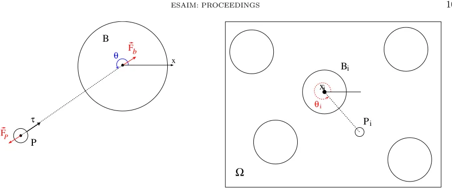
We consider a connected bounded and regular domain Ω ⊂ R2 and we denote by (Bi)i=1,...,N the rigid
particles, strongly included in Ω (see right in Fig 1). Bdenotes the whole rigid domain: B=∪iBi. The domain
Ω\B¯ is filled with Newtonian fluid governed by the Stokes equations. Here,µis the viscosity of the fluid and ff the external forces exerted on it. Since we consider a Newtonian fluid, the stress tensorσwrites
σ= 2µD(u)−pI, where D(u) = ∇u+ (∇u)
T
2 .
For the sake of simplicity we will consider homogeneous Dirichlet conditions on∂Ω. On the other hand, viscosity imposes a no-slip condition on the boundary∂B of the rigid domain.
Following [2], bacteria are modeled as spherical particles of constant radius Rb, each of which has an
asso-ciated point force, representing the force exerted by the flagella on the fluid. A force of same intensity but opposite sign is exerted on the particle, due to propulsion. Actually, in order to regularize the problem, the force applied by the flagellar bundle on the fluid is represented by a volume force densityfp supported in a ball P of small radiusRp and which center is placed at some constant distancedfrom the center of sphereB. The
propulsion force is directed radially outward from the center of the particle and has some orientation angleθ, measured from thex-axis, as shown in Fig. 1.
The total force exerted on the fluid by the flagellar bundle associated to the ith particle has a constant magnitudefp and will be denoted byFip:
Fip=−fpτi=
Z
Pi
fPi dx, with fpi =− fp meas(Pi)
FP Fb B x θ τ P
Ω
i i Pθ i
xi
B
Figure 1. Left: single bacterium, right: whole domain with inclusions
whereτiis given by the orientation angleθi. The total force exerted by the flagella on their associated particle Biwill be denoted byFib and is equal to−F
i
p, so that we can write:
Fib =fpτi=
Z
Bi
fbidx, with fbi= fp meas(Bi)
τi.
At the initial time the particles are distributed randomly over the fluid (without overlapping). The position of the center of theith particle is denoted by xi,vi andωi its translational and angular velocities.
We have to find the velocityu= (u1, u2) and the pressure fieldpdefined in Ω\B¯, as well as the velocities of the particlesV:= (vi)i=1,...,N ∈R2N andω:= (ωi)i=1,...,N ∈RN such that:
−µ∆u +∇p = ff in Ω\B,¯
∇ ·u = 0 in Ω\B,¯
u = 0 on ∂Ω,
u = vi+ωi×(x−xi) on ∂Bi, ∀i∈ {1, ..., N}.
(1)
The external forces considered on the fluid are gravity, and the forces exerted by the flagella, so that
ff =
X
i=1...N
fpiχip,
whereχi
pis the characteristic function associated to the ballPi. Finally, Newton’s second law of motion, written
here in the non-inertial regime, couples the equations:
Z Bi
fbi−
Z
∂Bi
σ·n = 0 ∀i,
Z
Bi
(x−xi)×fbi−
Z
∂Bi
(x−xi)×σ·n = 0 ∀i.
(2)
The motion of each bacteriumBi is then set by its instantaneous velocityu(x, t) =vi(t) +ωi(t)×(x−xi(t))
defined on∂Bi. On one hand, the centerxi of the particleBi follows the differential equation
˙
On the other hand the relative position of its corresponding flagellumPirotates with angular velocity ωi,i.e.
˙
θi(t) =ωi(t).
1.2.
Tumbling and chemotaxis
E. Coli performs chemotaxis by alternating running and tumbling, and biasing the duration of the runs. The run durations are exponentially distributed with a rate of average λ∼1 s−1 (see [19]). Therefore, we model tumbling through a Poisson process with variable intensity. The time spent tumbling is neglected, and the run timeTrunof each bacterium,i.e.the time elapsed between two tumbles, follows an exponential law of parameter
λ, which represents the tumbling frequency. This frequency varies depending on the surrounding environment of the bacterium, that is depending on if it is going in a favorable direction or not.
Letc be the concentration of the chemical attractant considered. A first simplified model for the tumbling frequency reads as:
λ(c) = 1−ε φ
Dc
Dt
, (3)
were Dc/Dtis the Lagrangian derivative ofcalong the trajectory of the bacterium, andφis the sign function. We could also use a model of the following, more realistic type, used in several earlier models (see for example [19]):
λ(c) = 1−ε φ
Z t
t−∆t
c(s)g(t−s) ds
where g(s) = 1 ifs≤∆t/4 and g(s) = −1/3 ifs >∆t/4. The latter model assumes that the bacterium has some kind of “memory” and adapts to a concentration derivative evaluated during some time step ∆t.
Although the swimming directions before and after a tumble are correlated, with a mean angle between both directions of∼60◦ [1, 19], we neglect this fact and in our model the bacterium randomly chooses a new orientation angleθ after each run.
1.3.
Oxygen dynamics
In this work we consider oxygen as the only chemoattractant in the bacteria’s environment. The dynamics of the oxygen concentration care described by the following equation:
∂tc+u· ∇c−Dc∆c=−g(c, B), (4)
where Dc is the oxygen diffusion coefficient, uthe fluid velocity and −g(c, B) is the sink term accounting for
the oxygen consumption by the bacteria. This term can be written as follows:
g(c, B) =κ f(c)χB,
where κis the volumic consumption rate (in oxygen molecules per second per volume of bacteria), χB is the
characteristic function for the “bacterial” domain, andc→f(c) modulates this rate, going to 1 whencis large, but vanishing asc is smaller than a critical value (in the simulations, we will use the functionf(c) =cfor the sake of simplicity).
Notice also that, as a feedback, the motion of the bacteria can be related to the oxygen concentration as follows: bacteria which do not consume enough oxygen loose their capacity of self-propulsing [4]. Therefore, the intensity of the self-propulsion forcefp is modulated by the so-called motility function r(c) which is equal
2.
The coupled fluid and rigid body problem
2.1.
Variational formulation over constrained spaces
Following what has been done in [12, 15], we establish a variational formulation of the continuous problem involving functions which are defined on the whole domain. In that way we will avoid working on the time dependent fluid domain, that would necessitate remeshing. This can be achieved by introducing rigid constraints into the functional spaces considered:
K∇ = u∈H01(Ω), ∇ ·u= 0 ,
KB =
u∈H1
0(Ω), ∀i∃(vi, ωi)∈R2×R; u(x) = vi+ωi×(x−xi) a.e. inBi .
Here K∇ is the space of divergence free functions defined on Ω, andKB is the space of functions which do
not deformB. The latter can also be written as follows:
KB =
u∈H01(Ω), D(u) = 0 a.e. inB .
The solution to the initial problem, defined on Ω\B¯, can be extended on the whole domain Ω by a function in KB: u(x,·) =vi+ωi×(x−xi) inBi∀i, and we still denote this extension byu.
Let (u, p) be the extended solution of the problem. On the one hand we write the incompressibility equation in its usual variational form. On the other hand we multiply the momentum equation by a test function euin KB, integrate it by parts over Ω\B¯, and then extend the integrals over Ω using the fact that ∇ ·u= 0 and
D(u) = 0 in KB. Finally, using the boundary conditions of the problem, we obtain the following variational
formulation (see [12]):
2µ Z Ω
D(u)·D(eu)− Z
Ω
p∇ ·eu =
Z
Ω
f·ue, ∀ue∈KB,
Z
Ω
q∇ ·u = 0, ∀q∈L2 0(Ω),
(5) where f = N X i=1
fbiχib+fpiχip, andL2
0(Ω) stands for the set ofL2 functions over Ω with zero mean value.
2.2.
Penalty method to enforce the rigid motion
In the last two decades, different methods have been designed to simulate the motion of rigid bodies in a viscous fluid. Let us mention two important methods:
• Another class of approaches relies on fictitious domain-type methods, which allow us to use Cartesian grids in the whole domain. The presence of the entities in the fluid is dealt with an iterative algorithm on an auxiliary field (composed of Lagrange multipliers) which warrants the rigid motion constraint of the particles (see e.g. [7, 8]). An alternative to this are penalty methods: the rigid motion constraint is obtained by relaxing a term in the variational formulation, which amounts to replace rigid zones by highly viscous ones (see [12, 23]). As rigid velocities are polynomials of degree 1, it is possible to take into account the rigid motion by combining the finite elements of the mesh that correspond to the rigid domain: this method is developped and studied in [20].
In this work, the penalty method will be used, mainly because of its ease of implementation.
Formulation (5) involves a solution and test functions defined in the constrained space of rigid motions onB. In order to relax this constraint and obtain a formulation adapted to a finite element discretization, we use a penalty method. This method has already been used in [15] to enforce the rigid motion constraint of particles in a fluid flow. It consists of considering the minimization problem over a constrained domain associated to (5) and relaxing the constraint by introducing a penalty term in the minimized functional. The added term is the following:
1 ε
Z
B
D(u) : D(u)
so thatD(u) goes to zero whenεgoes to zero andutends to a rigid motion inB. The variational formulation obtained is:
2µ Z Ω
D(u) : D(u) +e
2 ε
Z
B
D(u) : D(u)e − Z
Ω
p∇ ·eu = Z
Ω
f·eu, ∀eu∈H1 0(Ω),
Z
Ω
q∇ ·u = 0, ∀q∈L20(Ω),
(6)
It has been proven in [12] that, in this framework, the penalty method converges linearly inε, i.e.solution of problem (6)u converges to solution of problem (5)uasεvanishes, and the convergence is of order 1 in ε. We
refer to [18] for a detailed analysis of a scalar version of this problem, which provides an error estimate for the space-discretized problem at the orderε+h1/2.
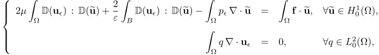
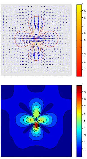
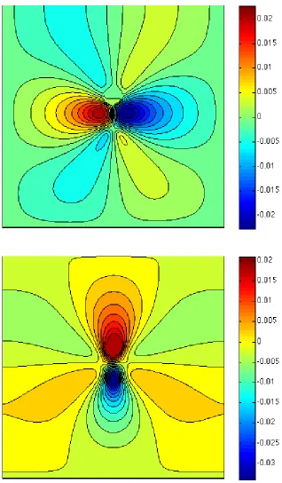
Let us look at a numerical simulation performed using the penalty method (here referred as Exp. 1, see Table 1, page 122). We have considered a square domain with one bacterium whose head B is placed at x= (0.5,0.6) and whose orientation is such thatθ= 3π/2. The variational formulation related to the penalty method (ensuring the rigid body constraint) allows us to compute the velocity field in the whole domain, using a finite element method: Fig. 2 and 3 highlight the influence of the self propulsion force and the rigid body constraint (note that the flow is considered to be at rest in absence of bacteria). See in particulara) the velocity field in the domain, b) the first component of the velocity field and c) the second component of the velocity field. The location of the flagellumP can be deduced from the second component of the velocity field, since it matches with the high peak negative value (the propulsion force being directed to the bottom); as a response, the high peak positive value of the second component of the velocity field matches with the head B of the bacterium.
3.
Time discretization
We denote by ∆t >0 the time step and for any function (x, t)→f(x, t), we denote byfnthe approximation
off(·, n∆t). At t=tn, the solid domain is denoted byBn =∪Bn
i. Fori= 1...N, theith particle is defined by
the positionxn
3.1.
A contact algorithm
Assuming, as we did in our model, that particle surfaces are smooth and that Stokes model is valid at any scale, it is known that contacts are not supposed to happen (see [6, 10]). Yet in actual simulations, collisions between particles are likely to occur. From a numerical point of view, it means that the spheres may overlap when their positions are updated after the velocity field computation. The treatment of possible overlap of the spheres is even more important in the case of dense suspensions. For that purpose we use a numerical method proposed by Maury in [17], where inelastic collisions between rigid particles are computed. It consists of projecting the velocity field onto some convex set depending on the current configuration, so that particles do not overlap. To be more precise, let us denote byXn:= (xni)i=1,...,N the position ofN bacteria (more precisely,
the position of their gravity centre) at timetn. Now we define the set
K(Xn) =V∈R2N, Dij(Xn) + ∆tGij(Xn)·V≥0,∀i < j , (7)
where
Dij(Xn) =
xni −xnj
−2Rb
denotes the signed distance between two spheresBi andBj and
Gij(Xn) =∇Dij= (...,0,−eij,0, ...,0,eij,0, ...), eij =
xj−xi
|xj−xi|
is the gradient of the distance.
In order to avoid overlapping, the following splitting procedure is proposed: in a first step, we solve the variational problem without taking into account the possible overlapping of the particles (thus defining an a priori velocity of the spheres), then compute the projection of this a priori velocity onto the set of admissi-ble velocities defined by (7). This projection is performed by an Uzawa algorithm on its saddle-point formulation.
The algorithm reads as follows: Assume that the position of the bacteria (Xn, θn
) is known at time tn.
We aim at determining the velocity field un in the fluid, the motion of the bacteria (Vn, ωn) and update the
position of the bacteria (Xn+1,θn+1):
i. Solve the variational formulation: find (un, pn)∈H01(Ω)×L20(Ω) such that
2µ Z Ω
D(un) : D(eu) +
2 ε
Z
B
D(un) : D(u)e − Z
Ω
pn∇ ·ue =
Z
Ω
fn·ue, ∀ue∈H1 0(Ω),
Z
Ω
q∇ ·un = 0, ∀q∈L2 0(Ω).
ii. Compute the a prioritranslational and angular velocity of the bacteria:
ˆ vni =
Z
Bn i
un(x) dx, ωni =
Z
Bn i
(x−xni)⊥·un(x) dx
Z
Bn i
|x−xni|2 dx
iii. Compute the admissible velocityVn as the projection of thea priorivelocity ˆVn:
V
n−Vˆn
2
= min
V∈K(Xn) V− ˆ Vn 2 .
iv. Update the position of the bacteria at timetn+1:
The interest in the procedure relies on the possibility to use any suitable solver for the computation of the dynamics. Contacts are handled at a second stage, without any consideration of the proper dynamics. At some point, it allows the use of any solver for the resolution of the dynamics problem: then the so-called predicted velocity field is projected onto the set of admissible velocity fields.
Let us give some comprehensive details on the contact algorithm and the effective procedure related to it. The numerical treatment of the constraint is based on an equivalent formulation of the minimization problem, as it is is treated as a saddle-point problem, by using the introduction of Lagrange multipliers:
(
Find (Vn,Λn)∈R2N×RN+(N−1)/2 such that
J(Vn, λ)≤ J(Vn,Λn)≤ J(V,Λn), ∀(V, λ)∈R2N ×RN+(N−1)/2 with the following functional:
J(V, λ) = 1 2 V− ˆ Vn 2 − X
1≤i<j≤N
λij (Dij(Xn) + ∆tGij(Xn)·V).
Notice that the number of Lagrange multipliers corresponds to the number of possible contacts. In particular, if there is no contact between particles i and j, then λij = 0 and the Lagrange multiplier is not activated;
conversely, if there is a contact between the two spheres, then λij may be positive and the corresponding
auxiliary field allows the velocity field to satisfy the no-overlapping constraint. The approximate reaction field Λn= (Λn
ij) is the dual component of a solution to the associated saddle-point problem. This problem is solved
by an Uzawa algorithm (see, e.g., [3]).
3.2.
Discrete tumbling
In order to simulate tumble for each bacterium, we need to time-discretise a Poisson process with variable intensity (i.e.the frequency of tumblingλ). For that purpose, we set ∆tT >0 a fixed time-step, and we define PT the probability of a bacterium to tumble at least one time during ∆tT. This probability can be computed
and depends on the values of ∆tT andλ:
PT(λ,∆tT) = 1−exp(−λ∆tT). (8)
Now, for each bacterium, the frequency of tumblingλvaries in time following (3). Therefore, the value of PT
also varies in time, depending on the sign of the lagrangian derivative of the concentration Dc/Dtevaluated by the bacterium along its trajectory. After each time-step ∆tT, each bacterium performs a random reorientation
(a tumble) with probability:
PT(c) = 1−exp
−
1−ε φ
Dc
Dt
∆tT
.
Note that with this procedure we neglect the fact that there can be more than one reorientation during ∆tT.
But this has no influence on the result as long as we neglect correlation between the directions before and after tumbling.
4.
Numerical results
4.1.
Chemotactic model (oxygen-bacteria model)
very much reduced. The CPU time is only due to contact handling and oxygen dynamics. The motion of the bacteria is obtained as follows:
• the norm of the bacteria velocity is prescribed, taken as a constant value;
• the direction of the bacteria is determined by the chemotactic response, including runs and tumbles. • thea priori velocity is corrected through contact handling.
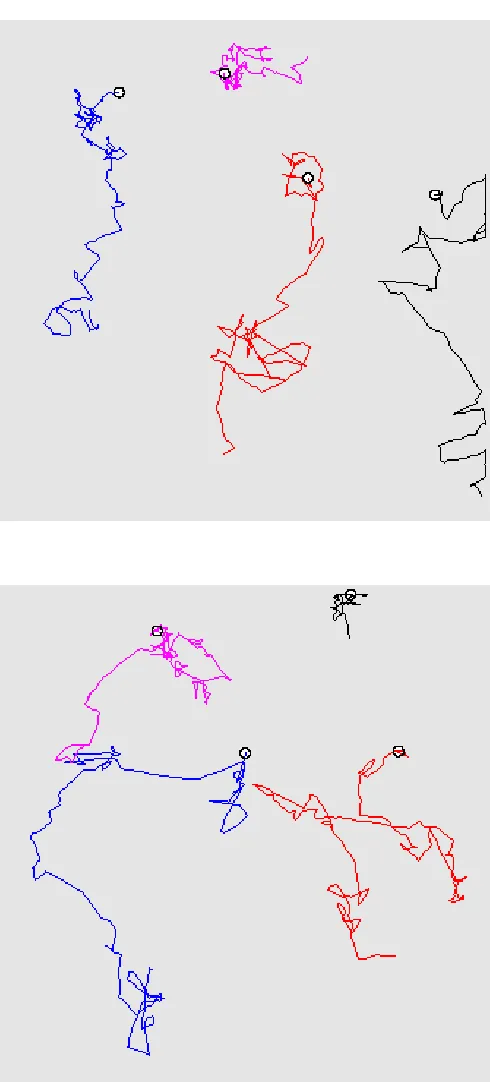
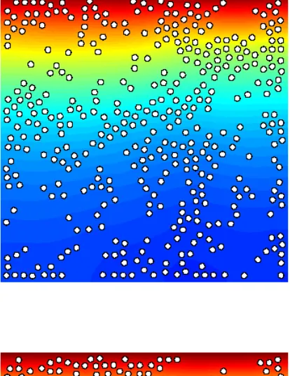
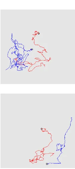
Fig. 4 provides results related to a numerical simulation referred asExp.2 (see Table 1 for the parameters). We may observe snapshots of the oxygen distribution and position of the microstructure (800 bacteria) at different times steps (1·∆t, 60·∆t and 400·∆t) in a square domain. During the whole simulation, the boundary conditions are the following: a Dirichlet boundary condition (c = 1) is imposed on upper boundary and a homogeneous Neumann condition is imposed on the other ones. At initial time, the oxygen distribution is homogeneous in space and the bacteria have been placed randomly in the domain. After one time step (Fig. 4-a)), we observe a local consumption of oxygen, which is larger where the density of bacteria is high. After 60 time steps (Fig. 4-b)), an oxygen gradient has appeared through the conjunction ofi) consumption of oxygen by the bacteria,ii) oxygen supply from the boundary modelling the fluid-air interface andiii) diffusion of oxygen into the whole domain. After 400 time steps (Fig. 4-d)), most of the bacteria have migrated towards the supply boundary, following the oxygen gradient. Notice also that, at final time, the oxygen concentration far from the supply boundary has increased because of the low density of bacteria. Interestingly, we can focus on the individual behaviour of bacteria: Fig. 5 represents the trajectories of some bacteria during all the simulation (the latest position is provided by the representation of the bacteria), which reveals the succession of runs and tumbles of the bacteria, leading to an average motion directed to the upper boundary modelling the air-fluid interface.
4.2.
Full model (oxygen-bacteria-fluid model)
Numerical tests have been performed with the full model. In the unit square domain, we have considered 400 bacteria in a Stokes flow. Chemotaxis and hydrodynamic interactions between the bacteria and the fluid are taken into account.
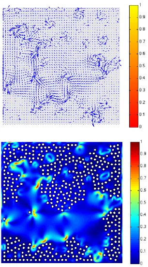
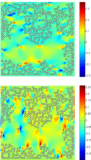
In this setting, the numerical simulation presented here refers toExp.3 (see Table 1 for the parameters). Fig. 6 provides snapshots of the oxygen distribution and position of the microstructure (400 bacteria) at different times steps (1·∆t, 200·∆t, 500·∆t and 2000·∆t). We may observe that some bacteria have succeeded in reaching the upper supply boundary while other bacteria have been trapped at the bottom: the latter is due to the fact that we imposed a zero-velocity of the fluid at the bottom only, so that the bacteria hardly move in this region. Fig. 7 shows the streamlines of the velocity fluid (t) and the norm of the velocity field (b) in the domain at timet= 2000·∆t. Fig. 8 shows the first component of the fluid velocity, the second component of the fluid velocity in the domain at timet= 2000·∆t; this allows to observe the effects of the propulsion forces on the fluid velocity and, as a response, on the bacteria. Fig. 9 represents the trajectories of some bacteria: it can be observed that the motion of the fluid now has a strong influence on the trajectories of the bacteria which tend to adapt to the oxygen gradient (via the run and tumble process) but are subject to the fluid flow.
References
[1] H.C. Berg, Random walks in biology,Princeton University Press, Princeton (1983).
[2] B.M Haines, I.S. Aranson, L. Berlyand and D.A. Karpeev, Effective viscosity of dilute bacterial suspensions: a two-dimensional model,Phys. Biol., 5 (2008)
[3] P. G. Ciarlet,Introduction `a l’analyse num´erique matricielle et `a l’optimisation, Masson, Paris (1990).
[4] L.H. Cisneros, R. Cortez, C. Dombrowski, R.E. Goldstein, J.O. Kessler, Fluid dynamics of self-propelled microorganisms, from individual to concentrated populations,Exp Fluids, 43:737–753 (2007).
Exp. 1 Exp. 2 Exp. 3 Domain (0,1)×(0,1) (0,1)×(0,1) (0,1)×(0,1)
Mesh
Vertices 22801 10201 10201 Triangles 45000 20000 20000
Bacteria
Number of individuals 1 800 400 Head radius [RB] 0.0335 0.0101 0.0101
Flagellum radius [RP] 0.0335 0.0101 0.0101
Distance head-flagellum [DB−P] 0.1342 0.0202 0.0303
Propulsion intensity [fp] 0.3355 2.0000 5.0000
Propulsion modulation [r(c)] − 1 1
Fluid solver
BC (lower boundary) u=0 − u=0 BC (other boundaries) u·n= 0 − u·n= 0
Oxygen concentration
Initial condition − c≡1 c≡1 BC (upper boundary) − c= 1 c= 1 BC (other boundaries) − ∇c·n= 0 ∇c·n= 0 Diffusion parameter [Dc] − 1.00 0.50
Consumption rate [κ] − 39.20 98.00 Consumption function [f(c)] − c c
Table 1. Parameters for the numerical simulations
[6] D. G´erard-Varet, M. Hillairet, Regularity Issues in the Problem of Fluid Structure Interaction, to appear in Arch. Rational Mech. Anal.
[7] R. Glowinski, T. W. Pan, T. I. Hesla, D. D. Joseph & J. P´eriaux, A fictitious domain approach to the direct numerical simulation of incompressible viscous flow past moving rigid bodies: application to particulate flow, J. Comp. Phys. 169, 363–427 (2001).
[8] R. Glowinski,Finite element methods for incompressible viscous flow, In: Handbook of Numerical Analysis, Vol. IX, P. G. Ciarlet and J.-L. Lions eds., Ed. North-Holland, Amsterdam (2003).
[9] F. Hecht, A. Le Hyaric, K. Ohtsuka, and O. Pironneau,Freefem++, finite elements softwarehttp://www.freefem.org/ff++/. [10] M. Hillairet, Lack of collision between solid bodies in a 2D constant-density incompressible flow,Communications in Partial
Differential Equations 32: 1345-1371 (2007).
[11] H. H. Hu,Direct simulation of flows of solid-liquid mixtures, Int. J. Multiphase Flow22(2), 335–352 (1996).
[12] J. Janela, A. Lefebvre, B. Maury, A penalty method for the simulation of fluid-rigid body interaction,ESAIM: Proc., 1:115–123 (2005).
[13] A. A. Johnson & T. E. Tezduyar,Simulation of multiple spheres falling in a liquid-filled tube, Computer Methods in Applied Mechanics and Engineering,134(3), 351–373 (1996).
[14] E. Lauga and T.R. Powers, The hydrodynamics of swimming microorganisms,Rep. Prog. Phys., 72 (2009)
[15] A. Lefebvre, Fluid-particle simulations with Freefem++,ESAIM: Proc., 18:120–132 (2007).
[16] B. Maury,Direct simulations of 2D fluid-particle flows in biperiodic domains, Journal of Computational Physics156, 325–351 (1999).
[17] B. Maury, A time-stepping scheme for inelastic collisions,Numerische Mathematik, 102(4):649–679 (2006).
[18] B. Maury, Numerical Analysis of a Finite Element / Volume Penalty Method,SIAM J. Numer. Anal. Volume 47, Issue 2, pp. 1126-1148 (2009).
[20] J. San Mart´ın, J.-F. Scheid, T. Takahashi & M. Tucsnak,Convergence of the Lagrange–Galerkin method for the equations modelling the motion of a fluid-rigid system, SIAM J. Numer. Anal.,43(4), 1539–1571, (2005).
[21] L. Turner, W.S. Ryu, H.C. Berg, Real-time imaging of fluorescent flagellar filaments,J. Bacteriol., 182(10):2793–2801 (2000).
[22] I. Tuval, L. Cisneros, C. Dombrowski, C. W. Wolgemuth, J.O. Kessler, Bacterial swimming and oxygen transport near contact lines,Proceedings of the National Academy of Sciences (USA) 102, 2277-2282 (2005).