The Evolution of the Local Induction Approximation for a Regular Polygon *

J.-S. Dhersin, Editor

THE EVOLUTION OF THE LOCAL INDUCTION APPROXIMATION FOR A

REGULAR POLYGON

Francisco de la Hoz

_{and Luis Vega}

Abstract. In this paper, we consider the so-called local induction approximation (LIA): Xt=Xs∧Xss,

where ∧ _{is the usual cross product, and s denotes the arc-length parametrization. We study its}

evolution, taking planar regular polygons ofM sides as initial data. Assuming uniqueness and bearing in mind the invariances and symmetries of the problem, we are able to fully characterize, by algebraic means,X(s, t)and its derivative, the tangent vectorT(s, t), at timestwhich are rational multiples of

2π/M2_{. We show that the values at those instants are intimately related to the generalized quadratic}

Gauß sums.

Résumé. Dans cette courte note, nous considérons l’approximation d’induction locale (communément appelée LIA, par ses initiales en anglais):

Xt=Xs∧Xss,

où∧_{symbolise le produit croisé habituel et s est le paramétrage par longueur d’arc. Nous étudions}

son évolution, en considerant des polygones plans réguliers à M côtés comme données initiales. En supposant l’unicité et en prenant en compte les invariances et les symétries du problème, nous sommes capables de caractériser complètement, par des techniques algébriques,X(s, t)et sa dérivée, le vecteur tangentT(s, t), à des instants tqui sont des multiples rationnels de 2π/M2_{. Nous montrons que les}

valeurs à ces instants sont intimement liées aux sommes quadratiques généralisées de Gauß.

1.

Introduction

We consider the initial-value problem for the binormal flow

X_t=κb_{, (1)}

∗_{This work was supported by MEC (Spain), with the project MTM2011-24054, and by the Basque Government, with the project} IT641-13.

1 _{Department of Applied Mathematics, Statistics and Operations Research, Faculty of Science and Technology, University of}

the Basque Country UPV/EHU, Barrio Sarriena S/N, 48940 Leioa, Spain. e-mail:[email protected]

2_{Department of Mathematics, Faculty of Science and Technology, University of the Basque Country UPV/EHU, Barrio Sarriena}

S/N, 48940 Leioa, Spain. BCAM – Basque Center for Applied Mathematics, Alameda de Mazarredo 14, 48009 Bilbao, Spain. e-mail:[email protected]; [email protected]

c

EDP Sciences, SMAI 2014

whereκis the curvature andb_{the binormal component of the Frenet-Serret formulae:}





T n b





s

= 



0 κ 0

−κ 0 τ

0 −τ 0



· 



T n b



; (2)

observe that the torsionτ does not appear explicitly in (1). This geometric flow can be expressed as

X_t=X_s∧X_{ss, (3)}

where∧is the usual cross-product,tis the time, andsis the arc-length parameter. It appeared for the first time in 1906 [11], and was rederived in 1965 [1] as an approximation of the dynamics of a vortex filament under the Euler equations. It is also known as the local induction approximation (LIA), or the Vortex Filament Equation (VFE). Since the tangent vectorT₌X_{s remains with constant length, we can assume that}T_∈S2 _{∀t, where} S2 _{is the unit sphere in}R3_{. Differentiating (3), we get the so-called Schrödinger map equation on the sphere:}

T_t=T_∧T_{ss. (4)}

Even if the solutions of (3)-(4) for an initial datum with a corner are well understood, both from a theoretical [2–5, 9] and from a numerical point of view [6, 7]; nothing had been done for more general initial data with several corners. However, in a recently submitted paper [8], we have considered for the first time the evolution of (3)-(4), taking a planar regular polygon ofM sides as the initial datum.

In this paper, we briefly announce some important results of [8]. Its structure is as follows. In Section 2, we apply a modified version of the Hasimoto transformation [10], in order to relate (3)-(4) and the nonlinear Schrödinger (NLS) equation. In Section 3, assuming uniqueness and relying on the fact that the NLS equation is Galilean-invariant, we are able to explain, by using generalized quadratic Gauß sums, the structure ofX_{(s, t)}

and T_{(s, t) at times t that are rational multiples of 2π/M}2_{. In Section 4, we actually recover} X_{(s, t) and} T_{(s, t) at those times. In Section 5, we simulate numerically (3)-(4), comparing the numerical results with}

those obtained algebraically in Section 4. Finally, in Section 6, we draw the main conclusions, pointing out some most recent research on the subject.

2.

The Hasimoto transformation

A central point of this paper is the natural connection between (3)-(4) and the NLS equation. Indeed, applying the Hasimoto transformation [10]:

ψ(s, t) =κ(s, t) exp

i Z s

0

τ(s′, t)ds′

, (5)

ψsatisfies

ψt=iψss+i ₁

2(|ψ|

2_+A(t))

ψ, (6)

whereA(t)is a certain real constant that depends on time. Nevertheless, for our purposes, it is not convenient to work with the torsionτ. Instead, we consider another version of the Frenet-Serret trihedron:





T e₁ e₂





s

= 



0 α β

−α 0 0

−β 0 0 

· 



T e₁ e₂



, (7)

for some vectorse_{1 and}e_{2 that form an orthonormal base with} T_{. In this case, the Hasimoto transformation}

takes the form

Bearing in mind (7), it is not too complicate to show [8] that this newψalso satisfies (6).

A very important property of the NLS equation is the fact that it is invariant by the Galilean transformations: ifψis a solution of (6), so is

˜

ψk(s, t)≡eiks−ik

2

t_ψ(s

−2kt, t), ∀k, t∈R_{. (9)}

3.

A solution of

_X

₌

_X

_∧

_X

for a regular polygon

AnM-sided regular polygon X_{(s,0) can be regarded as a planar curve whose curvature is a sum of Dirac}

deltas:

κ(s) = 2π M

∞

X

k=−∞

δ(s−2Mπk). (10)

SinceX_{(s,0)is planar, its torsion is zero; hence, we haveψ(s,0)≡κ(s), i.e.,}

ψ(s,0) = 2π M

∞

X

k=_−∞

δ(s−2πk

M ). (11)

ψ(s,0) satisfiesψ(s,0) = ˜ψM k(s,0)≡eiM ksψ(s,0),∀k∈Z. Hence, bearing in mind the Galilean transforma-tions (9) andassuming uniqueness,

ψ(s, t) = ˜ψM k(s, t)≡eiM ks−i(M k)

2

t_ψ(s

−2M kt, t), ∀k∈Z_,∀t∈R_{. (12)}

In general, the assumption of uniqueness plays an essential role along this paper. Indeed, both ψ(s, t) and ˜

ψM k(s, t)satisfy formally (6). Therefore, since both solutions of (6),ψ(s, t)andψ˜M k(s, t), have the same initial data att= 0, (12) holds only if uniqueness is guaranteed. This also implies that thej-th Fourier coefficients of ψ(s, t)andψ˜M k(s, t)are identical:

ˆ

ψ(j, t) = M 2π

Z 2π/M

0

e−iM js_{ψ(s, t)ds}

= M

2π Z 2π/M

0

e−iM js_ψ˜

M k(s, t)ds

= M

2π Z 2π/M

0

e−iM jsh_eiM ks₋i(M k)2_t

ψ(s−2M kt, t)ids

= M e−

i(M k)2_t

−iM(j₋k)(2M kt)

2π

Z 2π/M

0

e−iM(j−k)sψ(s, t)ds

=e−i(M k)2t−iM(j−k)(2M kt)ψˆ(j−k, t). (13)

This identity holds for allj andk. In particular, evaluating both sides atj=k:

ˆ

ψ(k, t) =e−i(M k)2_t ˆ

ψ(0, t), (14)

so ψcan be expressed as

ψ(s, t) = ˆψ(0, t)

∞

X

k=−∞

e−i(M k)2

t+iM ks_{, (15)}

whereψˆ(0, t)is a constant that depends on time and that has to be chosen in such a way that the corresponding

Moreover, combining (11) and (15), we get the following well-known identity:

∞

X

k=−∞

ei(M k)s≡2_Mπ

∞

X

k=−∞

δ(s−2πk

M ). (16)

Let us evaluate (15) at t = tpq ≡ (2π/M2)(p/q), where p ∈ Z, q ∈ N, and we can suppose without loss of generality thatgcd(p, q) = 1:

ψ(s, tpq) = ˆψ(0, tpq)

∞

X

k=_−∞

e−i(M k)2_2πp/(M2_{q)+iM ks}

= ˆψ(0, tpq)

∞

X

k=−∞

e−2πi(p/q)k2

+iM ks

= ˆψ(0, tpq) q−1

X

l=0 ∞

X

k=_−∞

e−2πi(p/q)(qk+l)2+iM(qk+l)s

= ˆψ(0, tpq) q−1

X

l=0

e−2πi(p/q)l2_{+iM ls} X∞ k=_−∞

eiM qks. (17)

Using the identity (16),

ψ(s, tpq) = 2π

M qψˆ(0, tpq) q−1

X

l=0

e−2πi(p/q)l2

+iM ls X∞

k=_−∞

δ(s−2M qπk)

= 2π

M qψˆ(0, tpq) q₋1

X

l=0 ∞

X

k=−∞

e−2πi(p/q)l2_{+iM l(2πk/M q)}

δ(s−2πk M q)

= 2π

M qψˆ(0, tpq)

∞

X

k=−∞

q−1

X

l=0

e−2πi(p/q)l2+2πi(k/q)lδ(s−2M qπk)

= 2π

M qψˆ(0, tpq)

∞

X

k=_−∞

q−1

X

m=0

q−1

X

l=0

e−2πi(p/q)l2

+2πi(m/q)l_δ(s

−2Mπk−

2πm M q)

= 2π

M qψˆ(0, tpq)

∞

X

k=_−∞

q₋1

X

m=0

G(−p, m, q)δ(s−2πk M −

2πm

M q), (18)

where

G(a, b, c) =

c−1

X

l=0

e2πi(al2+bl)/c, a, b∈Z_{, c∈}Z_{− {0}, (19)}

denotes a generalized quadratic Gauß sum. For our purposes, an important property of these sums is that

|G(−p, m, q)|=   

 

√_{q, ifq is odd,}

√_{2q, ifq is even andq/2}

≡mmod 2, 0, ifq is even andq/26≡mmod 2.

Therefore,ψ(s, t)has evolved fromM Dirac deltas in[0,2π)att= 0, toM q deltas in[0,2π)attpq, forqodd; andM q/2deltas in[0,2π)attpq, forqeven. Furthermore, from (20),

G(−p, m, q) =   

 

√_qeiθm, ifqis odd,

√

2qeiθm, ifqis even and q/2

≡m mod 2, 0, ifqis even and q/26≡m mod 2,

(21)

for a certain angle θm that depends on m (and, of course, onp and q, too). Introducing (21) into (18), and restricting ourselves tok= 0, i.e.,[0,2π

M), we conclude that

ψ(s, tpq) =                        2π

M√qψˆ(0, tpq) q−1

X

m=0

eiθm

δ(s−2M qπm), ifqodd,

2π Mqq₂

ˆ ψ(0, tpq)

q/2−1

X

m=0

eiθ2m+1_δ(s−4πm+2π

M q ), ifq/2 odd,

2π Mqq

2

ˆ ψ(0, tpq)

q/2−1

X

m=0

eiθ2mδ(s

−4πm

M q), ifq/2 even.

(22)

The coefficients multiplying the Dirac deltas are in general not real, except fort= 0andt1,2=π/M2. Therefore,

ψ(s, tpq)does not correspond to a planar polygon, but to a skew polygon with M q sides, for qodd; and to a skew polygon with M q/2 sides, for q even. Since the Dirac deltas are equally spaced at a time t = tpq, the length of the sides is the same. Finally,ψˆ(0, tpq)has to be determined in such a way that the polygon is closed.

4.

Recovering

_X

and

_T

from

_ψ

at

_t

₌

_t

Givenψ(s, t) =α(s, t) +iβ(s, t), recoveringT_,e_{1 and}e_{2from ψimplies integrating}

  T e₁ e₂   s =  

0 α β

−α 0 0

−β 0 0  ·   T e₁ e₂ 

. (23)

As we have seen in the previous section, at a timetpq= (2π/M2)(p/q), ψ(s, tpq) is a sum ofM q (ifqodd) or M q/2 (ifq even) equally spaced Dirac deltas, that corresponds to a skew polygon X_{(s, tpq) of M q or M q/2}

sides. To integrate (23), we have to understand the transition from one side of the polygon to the next one. In order to do that, we reduce ourselves, without loss of generality, to a certainψ formed by a single Dirac delta located ats= 0, i.e,ψ(s) = (a+ib)δ(s), so we have to integrate

  T e₁ e₂   s =  

0 aδ(s) bδ(s)

−aδ(s) 0 0

−bδ(s) 0 0  ·   T e₁ e₂ 

=δ(s)A·   T e₁ e₂ 

. (24)

The solution of this equation is





T₍₀+₎T e₁₍₀+₎T e₂₍₀+₎T



= exp(A)· 



T₍₀−₎T e₁₍₀−₎T e₂₍₀−₎T



where the rotation matrix exp(A_{)can be computed explicitly. Expressinga+ibin polar form, a+ib≡ρe}iθ_,

we get

exp(A_{) =}





cos(ρ) sin(ρ) cos(θ) sin(ρ) sin(θ)

−sin(ρ) cos(θ) cos(ρ) cos2_{(θ) + sin}2_{(θ) [cos(ρ)}

−1] cos(θ) sin(θ)

−sin(ρ) sin(θ) [cos(ρ)−1] cos(θ) sin(θ) cos(ρ) sin2_{(θ) + cos}2_(θ)



. (26)

Since the scalar product between two vectors is rotation-invariant, choosing the orthonormal base {T₍₀−_),

e₁₍₀−_), e₂₍₀−_{)} to form the identity matrix} I_{, we conclude from (26) that}T₍₀−_)·T₍₀+_{) = cos(ρ), i.e.,ρ is}

precisely the angle formed byT₍₀−_)andT₍₀+_).

Coming back to the general form ofψ, we have to integrate (24)M qorM q/2times to obtain a closed skew, i.e., non-planar polygon withM q orM q/2sides. But, according to (22), in[0,2π

M),

ψ(s, tpq) =                       

q₋1

X

m=0

(αm+iβm)δ(s−2_{M q}πm), ifqodd,

q/2−1

X

m=0

(α2m+1+iβ2m+1)δ(s−4πm_{M q}+2π), ifq/2odd,

q/2−1

X

m=0

(α2m+iβ2m)δ(s−4_{M q}πm), ifq/2even,

(27)

where

|αm+iβm|=ρ=        2π

M√qψˆ(0, tpq), ifqis odd,

2π Mqq₂

ˆ

ψ(0, tpq), ifqis even andq/2≡m mod 2,

0, ifqis even andq/26≡m mod 2,

(28)

so we conclude that, at any time tpq, the angle ρ between two adjacent sides is constant. Furthermore, the structure of the polygon is completely determined by the angles θm appearing in the generalized quadratic Gaussian sum, whereαm+iβm=ρeiθm.

LetM_{m be the rotation matrix corresponding to each(αm+iβm)δ(s) =e}iθmδ(s)in (22). Ifα

m+iβm≡0, M_{m is simply the identity matrix}I_{and can be ignored. Otherwise, from (26),}

M_m=





cos(ρ) sin(ρ) cos(θm) sin(ρ) sin(θm)

−sin(ρ) cos(θm) cos(ρ) cos2(θm) + sin2(θm) [cos(ρ)−1] cos(θm) sin(θm)

−sin(ρ) sin(θm) [cos(ρ)−1] cos(θm) sin(θm) cos(ρ) sin2(θm) + cos2(θm) 

. (29)

Therefore,



  

T₍2πk M q

+

)T e₁₍2πk

M q

+

)T e₂₍2πk

M q + )T    

=M_k·M_{k−1·. . .}M_1·M_0·





T₍₀−₎T e₁₍₀−₎T e₂₍₀−₎T



, ∀k∈N. (30)

In order that the polygon is closed, we have to choose ρin (28) in such a way thatT_,e_{1 and}e_{2 are periodic,}

i.e.,





T_(2π−₎T e_1(2π−₎T e_2(2π−₎T



= 



T₍₀−₎T e₁₍₀−₎T e₂₍₀−₎T



. (31)

Evaluating (30) at k=M q−1, (31) is equivalent to imposing that

M_{M q}

Let us define

M₌M_q−1·M_{q−2·. . .·}M_1·M_{0. (33)}

From (32), sinceM_{k+q ≡}M_{k ∀k,}M _{is an M-th root of the identity matrix}I_{. Moreover, it is also a rotation}

matrix that induces a rotation of2π/M degrees around a certain rotation axis. Therefore, we have to chooseρ in order that any of the following equivalent properties is satisfied:

Tr(M_{) = 1 + 2 cos(}2π

M), (34)

λ(M_{) ={1, e}2πi/M_{, e}−2πi/M_{}, (35)}

were Tr(M_)andλ(M_{)denote the trace and the spectrum of}M_{, respectively. We have worked with the trace,}

because it is algebraically easier. By means of a symbolic manipulator, it is not difficult to calculateρ, or more precisely cos(ρ), for some small values of q (v.g. q = 3,4,5,6,8), in order that (34) holds. The expressions obtained algebraically for cos(ρ)for those values of q strongly suggest that, for any q and for any pcoprime with it, the only possible real value for cos(ρ)is

cos(ρ) = (

2 cos2/q₍π

M)−1, ifqis odd,

2 cos4/q₍π

M)−1, ifqis even.

(36)

Although giving a universal proof that this formula holds for anyq seems complicate, we have checked it for a few more q. Moreover, it is absolutely in agreement with our numerical simulations (see [8] for more details). Therefore, we think that there is concluding evidence that this formula is valid for anyq. Hence, we are able to determine the value ofψˆ(0, tpq)in (15):

ˆ

ψ(0, tpq) =  

 M√q

2π arccos 2 cos

2/q₍π M)−1

, ifqis odd, Mqq₂

2π arccos 2 cos4/q( π M)−1

, ifqis even.

(37)

After obtaining completely ψ(s, tpq), we have integrated (23) up to a rigid moment, but the symmetries of (3)-(4) allow to compute the correct rotation of X _and T _{at t = tpq. Thus,} T _{may be fully determined by}

algebraic means, while we have been able to determineX_{up to a vertical movement.}

5.

Numerical experiments

We have simulated numerically a combination of (3) and (4),

(

X_t=T_∧T_s,

T_t=T_∧T_ss. (38)

using a fourth-order Runge-Kutta scheme in time, together with a pseudo-spectral discretization directly in space. More precisely, since we deal with periodic solutions ins∈[0,2π), we have simulated the evolution of

X_{= (X1, X2, X3)and}T_{= (T1, T2, T3)at N equally spaced nodessj= 2πj/N,j= 0, . . . , N −1.}

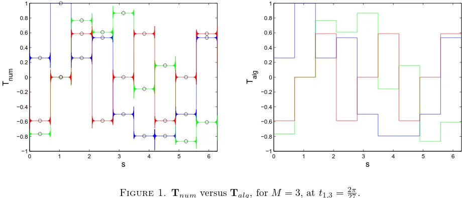
In Figure 1, we show the numerically obtained T_{num versus the algebraically obtained} T_{alg, conveniently}

rotated, for M = 3, s ∈ [0,2π), at t1,3 = 2₂₇π. We have taken 3×4096 frequencies. T1 appears in blue, T2

in green, T3 in red. In Tnum, the Gibbs phenomenon is clearly visible. Otherwise, the maximum discrepancy betweenT_{num and}T_{alg at the 27 points indicated by the black circles is6.3869·10}−9_.

With respect toX_{, we are able to fully determine it algebraically, except for a vertical movement. Therefore,}

0 1 2 3 4 5 6 −1

−0.8 −0.6 −0.4 −0.2 0 0.2 0.4 0.6 0.8 1

s

T num

0 1 2 3 4 5 6 −1

−0.8 −0.6 −0.4 −0.2 0 0.2 0.4 0.6 0.8 1

s

T alg

Figure 1. T_{num versus}T_{alg, forM = 3, att1,3=}2π

27.

conveniently, the heighth(t)of the mass center, which is precisely the mean of all the valuesX3(sj, t):

h(t) = 1 N

N₋1

X

j=0

X3(sj, t); (39)

remember that, thanks to the symmetries of the problem, the mean of both X1(sj, t) and X2(sj, t)is always zero. There is concluding numerical evidence that h(t)grows linearly witht, i.e.,

h(t) = h(2π/M

2₎

2π/M2 t=cMt, (40)

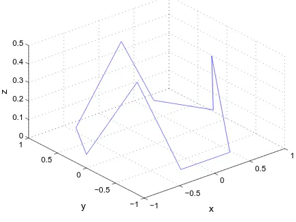
wherecM is a constant that depends on the number of initial sidesM. Furthermore, after adjustingcM, a very good agreement is also found between X_{num and} X_{alg. For instance, we have compared the} X_{alg and} X_num

corresponding to Figure (1). Takingc3= 0.7645,

kX_{alg+ (0,0, c3t1,3)−}X_numkL∞ = 3.9325·10−4.

Figure 2 showsX_{num. The nine equal-lengthed sides are clearly visible.}

6.

Conclusions and most recent research

In this paper, we have studied the evolution of (3)-(4), for a regular planar polygonal of M sides as initial datum. The algebraic calculations, backed by complete numerical simulations, suggest very strongly thatX_{(s, t)}

is a polygon at times which are rational multiples of2π/M2_{, i.e.,t}

pq= (2π/M2)(p/q), with the number of sides depending onq, whileT_{(s, t)is piecewise constant at those times.}

This paper raises multiple questions. We are currently conducting research on the subject and our priority is to give sense to our solutions from an analytical point of view. Moreover, while ourX_{(s, t), obtained algebraically}

for rational times, can be extended by continuity to all t ∈ R_{, it is not clear how to give sense to}T_{(s, t) at}

−1 −0.5

0 0.5

1

−1 −0.5 0 0.5 1 0 0.1 0.2 0.3 0.4 0.5

x y

z

Figure 2. X_{num, forM = 3, at t1,3=}2π

27.

References

[1] R. J. Arms and F. R. Hama. Localized-Induction Concept on a Curved Vortex and Motion of an Elliptic Vortex Ring.Phys. Fluids, 8(4):553–559, 1965.

[2] V. Banica and L. Vega. On the Stability of a Singular Vortex Dynamics.Commun. Math. Phys., 286(2):593–627, 2009. [3] V. Banica and L. Vega. Scattering for 1D cubic NLS and singular vortex dynamics.J. Eur. Math. Soc. (JEMS), 14(1):209–253,

2012.

[4] V. Banica and L. Vega. Stability of the Self-similar Dynamics of a Vortex Filament.ARMA, 210(3):673–712, 2013. [5] V. Banica and L. Vega. The initial value problem for the Binormal Flow with rough data. 2013. arXiv:1304.0996.

[6] T. F. Buttke. A Numerical Study of Superfluid Turbulence in the Self-Induction Approximation.J. Comput. Phys., 76(2):301– 326, 1998.

[7] F. de la Hoz, C. J. García-Cervera, and L. Vega. A Numerical Study of the Self-Similar Solutions of the Schrödinger Map. SIAM J. Appl. Math., 70(4):1047–1077, 2009.

[8] F. de la Hoz and L. Vega. Vortex Filament Equation for a Regular Polygon. 2013. arXiv:1304.5521.

[9] S. Gutiérrez, J. Rivas, and L. Vega. Formation of singularities and self-similar vortex motion under the localized induction approximation.Comm. PDE, 28(5–6):927–968, 2003.

[10] H. Hasimoto. A soliton on a vortex filament.J. Fluid Mech., 51(3):477–485, 1972.