www.hydrol-earth-syst-sci.net/16/4531/2012/ doi:10.5194/hess-16-4531-2012
© Author(s) 2012. CC Attribution 3.0 License.
Earth System
Sciences
Multi-objective optimization for combined quality–quantity urban
runoff control
S. Oraei Zare, B. Saghafian, and A. Shamsai
Department of Civil Engineering, Science and Research Branch, Islamic Azad University, Tehran, Iran Correspondence to: S. Oraei Zare ([email protected])
Received: 24 November 2011 – Published in Hydrol. Earth Syst. Sci. Discuss.: 16 January 2012 Revised: 6 October 2012 – Accepted: 10 October 2012 – Published: 3 December 2012
Abstract. Urban development affects the quantity and qual-ity of urban surface runoff. In recent years, the best manage-ment practices (BMPs) concept has been widely promoted for control of both quality and quantity of urban floods. How-ever, means to optimize the BMPs in a conjunctive quan-tity/quality framework are still under research. In this pa-per, three objective functions were considered: (1) minimiza-tion of the total flood damages, cost of BMP implementaminimiza-tion and cost of land-use development; (2) reducing the amount of TSS (total suspended solid) and BOD5 (biological oxy-gen demand), representing the pollution characteristics, to below the threshold level; and (3) minimizing the total runoff volume. The biological oxygen demand and total suspended solid values were employed as two measures of urban runoff quality. The total surface runoff volume produced by sub-basins was representative of the runoff quantity. The con-struction and maintenance costs of the BMPs were also esti-mated based on the local price standards. Urban runoff quan-tity and quality in the case study watershed were simulated with the Storm Water Management Model (SWMM). The NSGA-II (Non-dominated Sorting Genetic Algorithm II) op-timization technique was applied to derive the optimal trade off curve between various objectives. In the proposed struc-ture for the NSGA-II algorithm, a continuous strucstruc-ture and intermediate crossover were used because they perform bet-ter as far as the optimization efficiency is concerned. Finally, urban runoff management scenarios were presented based on the optimal trade-off curve using thek-means method. Sub-sequently, a specific runoff control scenario was proposed to the urban managers.
1 Introduction
Financial risks and health threats attributed to urban floods have always been challenging issues in urban planning of large cities. Urban runoff is often studied for planning pur-poses involved in runoff quality control, flood damage esti-mates and flood control management. Most of the measures aimed at prevention and/or crisis management during and af-ter the floods are parts of flood management. In recent years, a concept called BMPs, or alternatively known as the low impact development (LID), has been promoted in order to control the quality and quantity of urban floodwaters.
Zhen et al. (2004) used a heuristic optimization tech-nique that was coupled with a watershed model, i.e. the Annualized Agricultural Nonpoint Source Pollution model (AnnAGNPS), to minimize pollution cost under various combinations of BMPs. They used the AnnAGNPS model to assess the long-term reservoir performance subject to sed-iment deposition. Moreover, using the scatter search algo-rithm, the best locations for storage reservoirs were selected. Mejia and Moglen (2009) studied the effects of urban de-velopment and reduction of permeable areas by simulating water quantity and quality using a numerical model. They concluded that the resulting optimized landscapes provided a helpful understanding of the important role played by the spatial form of the urban pattern when trying to minimize impacts to water resources.
and Stroschein (2003) emphasized the use of a geographic information system (GIS) for site selection of structural and non-structural BMPs, including a combination of wetlands, ponds and natural channels. Baptista et al. (2007) investi-gated the use of BMPs with regard to production cost, en-vironmental impact and quantity control of floods. They de-scribed several steps of a decision making tool development, based on a multi-criteria procedure allowing a priori evalua-tion of the storm-water systems by aggregaevalua-tion of economic– financial–performance indicators. Based on their methodol-ogy, a decision aid tool was created to allow the choice of convenient project alternatives.
Lee et al. (2005) discussed methods to reduce pollution and runoff volumes in terms of some economic indicators. The study went further to evaluate and optimize the effects of wetlands in urban runoff quality control. Zhang et al. (2006) investigated the application of BMPs in urban runoff quantity control. They appliedε-NSGA-II algorithm to minimize the flood volume and cost of implementing three types of BMPs. They found their methodology as an efficient algorithm in decision making. Perez-Pedini et al. (2005) developed a dis-tributed hydrologic model of an urban watershed in the north-east United States and combined it with a genetic algorithm to determine the optimal location of infiltration-based BMPs for storm-water management. The results indicated that the optimal location and the number of BMPs was a complex function of watershed network connectivity, flow travel time, land use, distance to channel, and contributing area, thus re-quiring an optimization approach. A Pareto frontier describ-ing the trade-off between the number of BMPs (representdescrib-ing the project cost) and watershed flooding was developed.
Rodriguez et al. (2011) showed that the BMPs (combina-tion of pasture management, buffer zones, and poultry lit-ter application practices) were effective in controlling walit-ter. They used the NSGA-II to select and locate BMPs that effec-tively minimize nutrients pollution control cost by providing trade-off curves between the pollutant reduction and total net cost increase. Their optimization model generated a number of near-optimal solutions by selecting among 35 BMPs. For instance, total phosphorous (TP) could be reduced by at least 76 % while increasing the cost by less than 2 % in the entire watershed.
To our knowledge, previous studies have not reported multi-objective optimization of urban runoff control consid-ering coupled quality and quantity control. Flood quantity, cost of flood control, flood damages, capacity of sewerage systems in transmitting the floods or quality issues have been considered as single objectives in optimization frameworks of previous studies. Furthermore, assumptions used in the simulation of BMPs do not take all BMP characteristics into account. In reality, however, more parameters are required to properly characterize the BMPs. In this research, the effect of implementation of a number of urban runoff quantity and quality control measures are simulated using the Storm Wa-ter Management Model (SWMM) in a case study of a urban
watershed in Tehran. In an optimization framework, three objective functions are developed for optimum runoff quan-tity and quality control. The aerial coverage of each BMP in each sub-basin is considered as a decision variable. Op-timal decision variables are determined using the NSGA-II evolutionary optimization algorithm. The results of the pro-posed model are extracted in the form of the optimal trade-off curves. Each point on this curve represents a runoff manage-ment scenario.
2 Characteristics of the case study
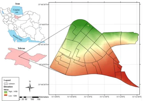
In recent years, Tehran, the capital of Iran, has been rapidly developing without due consideration of the adverse impacts on the environment and the water cycle. This has resulted in a wide range of challenges and obstacles in water sup-ply and sanitation infrastructures. Integrated runoff quality and quantity management is a necessity as the city grows. At least a number of times each year, Tehran residents must cope with excessive runoff impeding the traffic and causing damage to properties. The last deluge came in April 2012, causing tremendous traffic as well as breaking some flood wall protections. The urban flood waters with degraded qual-ity also end up in the southern part of the cqual-ity where they are used for irrigation. Thus, implementation of integrated flood management to deal with quantity and quality issues is vital. In this paper, a relatively small part of the northwest of Tehran is selected for the case study. This area is located downstream of Kan and Vardij Rivers, limited by Alborz Mountains in the north, Kan River in the east, Tehran–Karaj highway in the south and Vardavard Forest in the west. The highest elevation is 1459 m above mean sea level, while the lowest is 1264 m. This urban subarea of about 670.2 hectare was divided into 32 sub-basins (Fig. 1). The 5-yr design rain-fall subject to an observation-based temporal pattern is used in this research.
3 Methodology
As stated before, the main objective of this study is optimiza-tion of urban runoff control considering coupled quality and quantity aspects. Specifically, the expected output of the pro-posed approach will be the optimal level and layout of the land allocated to each studied BMP. The procedure is de-scribed below.
3.1 Data requirement
Fig. 1. Location of the study area in the country and within the Tehran province.
3.2 Hydraulic, hydrologic and quality modelling using SWMM
In this study, SWMM was employed to simulate quan-tity/quality hydrologic and hydraulic routing of urban runoff. SWMM has been developed by the USEPA (United State En-vironmental Protection Agency). SWMM (version 5.0.021) is a distributed on-site model primarily developed for urban areas. The model is capable of handling both water quantity and quality routing. Typical urban drainage network compo-nents such as manholes, underground pipes, storage units, di-viders, orifices, weirs, and open channels may be introduced within the SWMM (Huber and Stouder, 2006). In SWMM, hydrologic modelling is initiated by the definition of sub-basin characteristics as well as rainfall and pollution proper-ties. Sub-basins are simulated as nonlinear reservoirs while the output hydrograph is routed via kinematics wave (KW) or dynamic wave (DYW) approaches within the water con-veyance system.
In this study, the SCS curve number (CN) method was se-lected to determine infiltration losses. The CN method was adopted since the runoff depth may be expressed in terms of readily available land-use and hydrologic soil group maps. The CN method has been embedded into various watershed models for flood analysis, water quality and quantity mod-elling and land-use optimization (e.g. Yeo and Guldmann, 2010; Soulis and Valiantzas, 2012). There have been contin-uous efforts to modify the CN values under different physio-graphic and climatic conditions (Arnold et al., 1998).
Furthermore, flood routing was performed using the kine-matics wave method (Guo and Urbonas, 2009; Cheng, 2011). The kinematics wave method uses the normal flow assump-tion for routing flows through the conveyance system.
Pollutant loads vary depending on the characteristics of the catchment surfaces. From the surface, the pollutants will travel to the waterways and water bodies via surface runoff
(Hossain and Imteaz, 2009). Storm-water pollutant models are viewed as two stage processes: (1) gradual increase in dry air pollutants over the land with various uses, and (2) washing of the pollutants from the ground during rainfall. In SWMM, a pollutant model has been developed and inte-grated with the runoff model. The model will first estimate the pollutant build-up during the antecedent dry days (the days without rain) and then simulates the transport of the pollutants to the waterways and receiving water bodies by the surface runoff (Hossain et al., 2010).
3.2.1 Pollutant build-up model
Pollutant accumulation on catchment surfaces is a function of the number of preceding dry weather days. Pollutant build-up that accumulates over a land-use category is described (or “normalized”) by either a mass per unit of sub-basin area or per unit of curb length. The amount of build-up is a func-tion of the number of preceding dry weather days (Rossman, 2010; Egodawatta et al., 2009) as follows:
B=minC1, C2, tC3, (1)
whereB is the pollutant build-up (kg m−1) (mass per length curb),C1is the maximum build-up possible (kg m−1) (mass per length curb),C2is the build-up rate constant kg
mdayC3
, t is the number of preceding dry weather days, and C3 is the time exponent (dimensionless). In this research, the curb length is 100 m. The values of build-up coefficients (C2 andC3) were determined based on the relationship between build-up amounts with antecedent dry weather days for dif-ferent land uses and difdif-ferent quality indicators on the exper-imental data (Egodawatta, 2007).
3.2.2 Pollutant wash-off model
Pollutant wash-off is significantly influenced by the avail-able pollutants on the catchment surfaces. Pollutant wash-off from a given land-use category occurs during wet weather periods (Egodawatta, 2007), as expressed by
W=B1qB2M, (2)
where W is the wash-off load in units of mass per hour (kg h−1), B1 is the wash-off coefficient
mm h
−B2 h−1
, B2is the wash-off exponent (dimensionless),q is the runoff rate (mm h−1), andMis the pollutant build-up in mass unit (kg) (Giron´as et al., 2009).
In Eq. (2),B1andB2were determined based on the rela-tionship between wash-off load and pollutant build-up WM
andq on experimental data (Egodawatta, 2007; Hossain et al., 2010).
Table 1. Build-up and wash-off parameters (Tajrishi and Malekmohammadi, 2009).
Equation
Land use
of Low density High Density Industrial Other pollution Parameter C1 C2 C1 C2 C1 C2 C1 C2
Build-up TSS 2.98 0.9834 74.5 3.0694 193.7 9.1635 59.6 1.9817 BOD5 1.49 0.00517 2.235 0.01034 3.725 0.02682 1.639 0.00596
Parameter B1 B2 B1 B2 B1 B2 B1 B2
Wash-off TSS 0.4 2 0.7 2.2 0.3 2.5 0.1 1.7 BOD5 0.02 0.2 0.09 0.4 0.1 0.7 0.01 0.05
In this research, the coefficients in Eqs. (1) and (2) are pre-sented by Tajrishi and Malekmohammadi (2009) for the city of Tehran (Table 1), and BOD5 and TSS quality indicators are of primary concern.
3.3 Selection of the BMPs
There are several varieties of BMPs that can be used on a site. However, not all BMPs are suitable for all condi-tions. Therefore, it is important that the feasibility and con-straints are identified at an early stage in the design process. The restrictions in choosing appropriate BMPs are land-use characteristics, site characteristics, catchment characteristics, quantity and quality performance requirements, amenity and environmental requirements. The selected BMPs applied in this paper consist of rain barrels, porous pavement, and bio-retention. First, bio-retention was selected due to the great need for expanding the green space in the city of Tehran. Sec-ond, porous pavement is a feasible BMP for parking, court-yard houses and sidewalk areas. Third, rain barrels are suited to urban buildings and can supply a portion of non-potable water.
3.3.1 Porous pavements
Porous pavements are sustainable drainage systems (SUDS) for pedestrian and/or vehicular traffic, allowing rainwater to infiltrate through the surface and into the underlying lay-ers. The water is temporarily stored before infiltration into the ground, reuse, or discharge to a watercourse or other drainage system. Pavements with aggregate sub-bases can provide good water quality treatment. The three principal system types are described in Fig. 2.
Type A reflects a system where all the rainfall passes through the sub-structure into the soils beneath. In a Type B system, a series of perforated pipes at formation level will convey the portion of the rainfall that exceeds the infiltra-tion capacity of the sub-soils to the receiving drainage tem. There is no infiltration in a Type C system, and the sys-tem is generally wrapped in an impermeable, flexible mem-brane placed above the sub-grade. Once the water has filtered through the sub-base, it is conveyed to the outfall via perfo-rated pipes or fine drains (Woods-Ballard et al., 2007).
Fig. 2. Porous pavement system (Woods-Ballard et al., 2007).
3.3.2 Bio-retention
Bio-retention areas, also referred to as bio-retention filters or rain gardens, are structural storm-water controls that capture and treat storm-water runoff caused by more frequent rainfall events. Excess runoff from extreme events is passed forward to other drainage facilities. The water volume is treated using soils and vegetation in shallow basins or landscaped areas to remove pollutants. The filtered runoff is then both collected and returned to the conveyance system or, if site conditions allow, infiltrated into the surrounding soil. Part of the runoff volume will be removed through evaporation and plant tran-spiration. Suitable flow routes or overflows are required to safely convey water in excess of the design volumes to ap-propriate receiving drainage systems (Fig. 3).
3.3.3 Rain barrels
[image:4.595.309.546.95.352.2]Fig. 3. Plan schematics of a typical on-line bio-retention area (Woods-Ballard et al., 2007).
3.4 Structure of the multi-objective optimization model
3.4.1 Decision variables
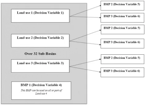
Decision variables for each sub-basin consist of rain barrel area (BMP1), porous pavement area (BMP2), bio-retention area (BMP3) and different land-use areas including industrial (land use 1), high density residential (land use 2) and low density residential (land use 3). Since there are 32 sub-basins within the study area, the optimization problem has a total of 192 decision variables (Fig. 4). Miscellaneous land-use area representing parks and green areas (land use4) is not considered as a decision variable; it is simply determined by subtracting the total areas of land use 1 to 3 from the sub-basin area.
3.4.2 Objective functions
Three objective functions were considered in this study: (1) minimization of the total flood damages, cost of BMP imple-mentation and cost of land-use development; (2) reducing the amount of TSS and BOD5, representing the pollution char-acteristics, to below the threshold level; and (3) minimizing the total runoff volume. The objective functions may be ex-pressed as follows:
F1=min 32
X
i=1 3
X
j=1
costIij
+
4
X
j=1
CjLALj
+10.13A0.7ij3+costD (3)
F2=min np
X
p=1 32
X
i=1
Ctip+max Con ave p Constp−1,0
!
×1010
!!
(4)
F3=min 32
X
i=1 Ri
!
, (5)
where
[image:5.595.52.284.66.191.2]costIij=20722.3Aij1+16.055Aij2−432 (6)
Fig. 4. The schematic of decision variables in each chromosome.
costD= nflood
X
f=1
3.28×h3f−22.9×h2f+51.2×hf+2
(7)
hf =βfp∀f (8)
βf =
s
Sf
2Bf (9)
Ci=
" 3 X
j=1
cjrALj+cr4 ATi −
3
X
j=1 ALj
!#
ATi (10)
Cin=
" 3 X
j=1
cjnALj+c4n ATi −
3
X
j=1 ALj
!#
ATi (11)
∀f =fnSWMMAij1j3=1 , Aij23j=1,
Aij3j=4 , hALji 4
j=1 , Ci, C n i
32
i=1
)
(12)
and
Conavep =
32
P
i=1
Ctip×ATi 32
P
i=1 ATi
. (13)
The objective functions are subject to the following con-straints:
2
X
k=1
ALj =ALj , i=1,2, ...,32, j=1,2,3 (14)
0≤Aij a≤ATi − 3
X
j=1
Table 2. Construction cost of different land uses.
Land use Cost value per one
square meter (USD)
Low density residential 4000
High density residential 8000
Industrial 2000
[image:6.595.357.497.83.148.2]Other (playground, park, ...) 500
Table 3. Implementation cost of BMPs.
BMP Cost (in USD)
Rain barrel C=2936×V−432
Bio-retention C=18.5×V0.7 Porous pavement C=65 000×A
Vis the volume of the BMP in cubic feet andAis the area of the BMP in acres.
0≤ 3
X
k=1
Aij1≤0.6× 3
X
j=1
ALj , i=1,2, ...,32, j=1,2,3 (16)
0≤ 3
X
k=1
Aij2≤0.4× 3
X
j=1
ALj , i=1,2, ...,32, j=1,2,3
, (17)
where
– i: refers to sub-basin number;
– j: refers to land-use type; – k: refers to BMP type;
– ALj: total area ofj-th land use (m2);
– CjL: cost of developingj-th land use (Table 2); – costIij: BMP implementation cost over thej-th
land-use type in thei-th sub-basin (details of the costs are given in Table 3);
– ATi : total area of thei-th sub-basin (m2); – costD: the cost of flood damage (in $);
– Aij k: area of thek-th BMP over thej-th land use in the i-th sub-basin (m2);
– nflood: total number of flood nodes;
– f: refers to the flooding nodes in each sub-basin; – hf: water level at thef-th flooding node (m);
– βf: a coefficient to determine volume given the height at thef-th flooding node;
[image:6.595.355.502.186.254.2]– ∀f: runoff volume at thef-th flooding node (m3);
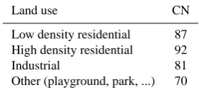
Table 4. Curve number (CN) of different land uses.
Land use CN
Low density residential 87
High density residential 92
Industrial 81
Other (playground, park, ...) 70
Table 5. Runoff coefficient of different land uses (ASCE, 1970).
Land use C (%)
Low density residential 50
High density residential 60
Industrial 70
Other (playground, park, ...) 20
– Sf: sub-basin slope at thef-th flooding node (%); – Bf: sub-basin width at thef-th flooding node (m); – cjn: curve number attributed to the j-th land use
(Ta-ble 4);
– Cin: average curve number of thei-th sub-basin; – cjr: runoff coefficient attributed to thej-th land use
(Ta-ble 5);
– Ci: runoff coefficient of thei-th sub-basin; – f (SWMM()): SWMM simulation model;
– Conavep : average concentration value of pollutant “p” over the entire basin (mg l−1);
– Constp: threshold (standard) concentration value of pol-lutant “p” (mg l−1);
– np: number of pollutants involved in the simulation; – Ctip: concentration of the pollutant “p” over thei-th
sub-basin (mg l−1); and
– Ri: runoff volume in thei-th sub-basin (m3).
[image:6.595.87.245.194.251.2]Fig. 5. The process leading to the optimal trade-off curve.
in Eq. (1). The cost of flood damage was determined using Eq. (7). Based on the quality simulation results, TSS and BOD5 values at each node were determined and compared with the threshold values. If the simulated values exceeded the thresholds, the loss function was determined based on the second term in Eq. (4). The total volume of runoff produced in all flooded nodes constitutes the total amount of runoff, as in Eq. (5).
According to Eq. (16), the covered area of BMP1 over land use 1, 2 and 3 in each sub-basin should be less than 60 % of the total sub-basin area. According to Eq. (17), total BMP2 covered area over land use 1, 2, and 3 in each sub-basin should be less than 40 % of the total sub-sub-basin area.
[image:7.595.310.544.64.229.2]A trade-off curve among the objectives was then extracted that contains various control scenarios. Figure 5 shows the process to arrive at the optimal trade-off curve. It should be noted that the values of the first, second and third objective functions are in dollars, kilograms and cubic meters, respec-tively. According to Eq. (4), the value of the second term in the second objective function is dimensionless. This term is associated with the penalty function.
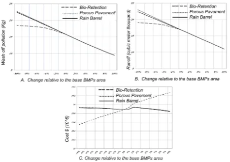
Fig. 6. BMP efficiencies: (A) in terms of runoff quantity control, (B) in terms of runoff quality control, and (C) on the damage cost.
3.5 Non-dominated Sorting Genetic Algorithm (NSGA-II)
A number of multi-objective evolutionary algorithms (MOEAs) have been proposed in the last two decades. The NSGA-II is one of the promising MOEAs and has been successfully applied in many engineering fields. The initial NSGA proposed by Srinivas and Deb (1994) could locate multiple Pareto-optimal solutions in one simulation run for multi-objective optimization problems. The NSGA-II is an improved version of the NSGA, developed to address issues of computational complexity as well as to provide an explicit mechanism for diversity preservation (Deb et al., 2000). The NSGA-II algorithm consists of five operators: initialization, fast non-dominated sorting, crossover, mutation and the eli-tist crowded comparison operator. A major difference be-tween the NSGA-II and other EAs is the method of opera-tor selection. The NSGA-II uses the non-dominated sorting and ranking selection with the crowded comparison opera-tor (Deb et al., 2000). This model has three new innovative aspects (Chang and Chang, 2009):
1. Fast non-dominated sorting: The fast non-dominated sorting approach has a better book-keeping strategy to speed up the non-dominated sorting process and reduce the computation complexity.
Fig. 7. Results of the last generation in the NSGA-II.
3. Crowded comparison operator: This operator guides the selection process at various stages towards a uniformly spread-out Pareto-optimal front. The crowding distance is applied to select one with a greater crowding dis-tance from two individuals in the same front. The elitist crowded comparison operator combines offspring pop-ulation members with parent poppop-ulation in the selection process that significantly speeds up to capture the pre-viously found nice solutions.
4 Results and discussion
One criterion for selection of the appropriate BMP is the suit-ability of implementation in the selected land use and its ef-fect on the runoff quantity and quality. In this section, the effect of each BMP on the runoff quantity and quality con-trol is described first. Then, the superior scenario for runoff quantity and quality control by means of a multi-objective optimization algorithm will be discussed.
4.1 Effect of BMPs on runoff quality and quantity control
Suitable definition of objective functions in determining the optimal solution is quite critical. In this study, the sensitivity of each objective function was assessed. Since the decision variables are the level of coverage for each BMP, changes in the levels were enforced. For this purpose, the proposed values in the Tehran master plan were used as the base values while the lower and upper ranges were 10 % less than and greater than the base values, respectively.
[image:8.595.57.285.64.222.2]Based on Figs. 6 to 8, rain barrels and porous pavement have similar performances in reducing the quantity and pol-lution of flood. An increased level of coverage is desirable in improving the runoff quality while reducing its quantity, despite increased construction and operation costs. Accord-ing to these figures, porous pavement and rain barrels would have a stronger effect on improving the quality and quantity
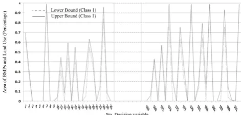
Fig. 8. Variation of decision variable in class 1 based on thek-means method.
Fig. 9. Flood hydrographs at the outlet for each class.
(the second and third objective functions) of runoff compared with the bio-retention.
The degree of improvement on the second and third ob-jective functions due to the increase in the BMP coverage levels is similar. However, bio-retention is more suitable for pollution and runoff volume reduction than the other two BMPs. The variation of the first objective function (construc-tion and opera(construc-tion costs) versus BMP coverage area is illus-trated in Fig. 6c. As it is observed, the costs of bio-retention and porous pavement change slightly compared to that of the rain barrels.
4.2 Sensitivity analysis to combined selection of decision variables
[image:8.595.312.545.235.392.2]Table 6. Sensitivity analysis in variable selection after 200 generations.
Mean Standard deviation
Variable Cost Runoff Pollution Cost Runoff Pollution
($)×109 (m3) (kg) ($)×109 (m3) (kg)
BMPs & land uses 1.05 1700 4.94 1.65 3000 19.61
Land uses 0.154 97.2 0.25 4.83 10 653 8.78
[image:9.595.140.460.205.365.2]BMPs 101.40 1362 0.22 172.85 3320 0.39
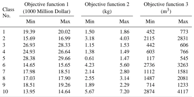
Table 7. Range of variation of objective functions in each class.
Class
Objective function 1 Objective function 2 Objective function 3
No. (1000 Million Dollar) (kg) (m
3)
Min Max Min Max Min Max
1 19.39 20.02 1.50 1.86 452 773
2 15.69 16.99 3.18 4.03 2115 2831
3 26.93 28.33 1.15 1.53 442 606
4 24.93 26.64 1.38 1.49 603 766
5 28.38 29.66 0.61 1.47 117 545
6 14.65 15.65 4.23 5.60 2736 3263
7 17.98 18.51 2.14 2.80 1112 1581
8 17.03 17.90 2.55 3.14 1487 2081
9 18.51 19.26 1.89 2.29 714 1233
10 13.95 14.64 5.67 7.20 2874 4117
the second and third objective functions under combination A was more than those of the B and C combinations. Thus, only combination A was further studied.
4.3 Convergence criteria
To determine the optimal trade-off between the objective functions, the maximum number of iterations must be spec-ified. The optimization algorithm was run for different num-bers of iterations. The results are shown in Fig. 7 for 40 to 200 iterations. It is seen that the variation of the objective functions between 160 and 200 iterations is negligible. So, the number of iterations needed for arriving at optimal deci-sion variables as well as optimal trade-off was set to 200.
For convergence of the trade-off curves, the criterion pro-posed by Chen et al. (2007) was adopted. In this criterion, the distribution of the production solution set and the maximum number of non-dominate solutions located on the trade-off curve are considered. Based on the cumulative distance val-ues of each solution, convergence criterion may be presented as follows:
DM=
db=de=
n−1
P
i=1
|di−d|
db+de+(n−1) d
, (18)
wheredbanddeare extreme values on the converged trade-off curves, di is the cumulative distance value of each
Table 8. Number of flooded nodes in each class.
Class Number of flooded nodes
1 4
2 4
3 0
4 4
5 0
6 5
7 4
8 4
9 4
10 16
solution on the trade-off curves, d is the average value of cumulative distance solutions, andnis the number of points on the converged trade-off curves.
The NSGA-II algorithm convergence condition is met when the criterion value is as close to zero as possible. The criterion for NSGA-II was determined as 0.4.
4.4 Classification of optimal trade-off curves
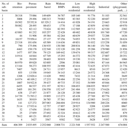
[image:9.595.361.495.408.542.2]Table 9. Optimal level of coverage (km2) associated with class 3.
No. of Bio- Porous Rain Without Low High Other
sub- retention pavement barrel BMPs density density Industrial (playground,
basin residential residential park, ...)
1 38 318 75 886 149 609 36 787 105 160 91 776 51 103 52 561
2 3008 29 496 100 213 79 083 83 383 52 220 60 687 15 510
3 18 502 55 552.8 83 329.2 14 416 61 028 54 191 23 663 32 918
4 58 082 28 495 88 653 1770 17 188 43 859 45 983 69 970
5 71 82 112 73 624 82 393 112 585 60 713 62 520 2382
6 63 883 81 232 103 257 22 428 60 482 40 838 101 760 67 720
7 44 51 908 49 384 62 264 60 639 29 037 72 288 1636
8 16157 75 950.4 27 137 97 256 74 053 31 570 84 253 26 624
9 23 318 101 656 65 589 114 636 69 851 51 032 133 258 51 059
10 790 175 496 136 935 130 380 200 834 86 140 151 766 4861
11 4463 158 178 122 540 132 120 181 258 35 206 178 980 21 856
12 1477 107 356 79 125 169 442 139 674 99 317 102 687 15 722
13 14 914 44 844 67 749 15 293 44 372 50 270 27 807 20 351
14 39 39 039 38 603 30 919 19 330 33 121 55 063 1086
15 84 970 89 820 83 005 2506 35 081 53 091 87 164 84 965
16 13 164 58 273 108 555 24 908 43 416 72 635 67 073 21 776
17 7407 7625 24 711 13 957 8613 8510 24 157 12 420
18 855 13 558 19 045 34 143 13 244 24 572 24 368 5417
19 1268 12 820.4 11 620 9992 7432 21 314 3305 3649
20 14 974 40 109.2 17 233 50 484 22 256 31 393 46 624 22 527
21 1807 54 922.8 39 437 49 733 37 352 54 909 45 046 8593
22 6455 86 537 151 197 82 911 106 653 106 035 90 837 23 575
23 2405 181 291 156 558 152 147 241 484 57 323 174 626 18 968
24 638 27 457 21 877 26 128 25 380 29 644 17 002 4074
25 14 739 71 593.2 19 895 113 273 65 438 27 769 85 776 40 517
26 1635 30 019 36 785 57 361 40 055 42 003 34 432 9310
27 141 127 272 207 083 266 604 219 914 134 900 240 226 6060
28 5114 17 933.6 12 757 17 897 28 927 3208 12 699 8867
29 32 17 656 35 651 33 860 42 923 24 577 18 668 1031
30 25 27 859 27 692 32 324 10 612 42 159 34 250 879
31 7612 60 121 89 653 42 014 35 826 60 592 84 032 18 950
32 4 3427 3567 9302 7105 3628 5397 170
Sum 406 309 2 035 495 2 252 068 2 008 731 2 221 548 1 557 552 2 247 500 676 004
k-centroids, one for each cluster. These centroids should be placed in a cunning way because different locations produce different results. A better choice is to place them as far away from each other as possible. The next step is to take each point belonging to a given data set and assign it to the near-est centroid. When no point is pending, the first step is com-pleted and an early grouping is done. At this point, we need to re-calculateknew centroids as barycenters of the clusters resulting from the previous step. After we have theseknew centroids, a new binding between the same data set points and the nearest new centroid is performed in a loop. As a re-sult, one may notice that thekcentroids change their location step by step until centroids do not move any more. The clus-tering algorithm aims at minimizing the following objective function:
J=
k
X
j=1 n
X
i=1
x
(j ) i −cj
2
, (19)
where
x
(j ) i −cj
2
is a chosen distance measure between a data pointxi(j )and the cluster centrecj, andjis an indicator of the distance ofndata points from their respective cluster centres.
Fig. 10. Comparison of scenarios based on the rank of objective functions.
class representative. Based on the selected classes, the range of variation of decision variables was determined. For exam-ple, Fig. 8 shows the variation range of decision variables as-sociated with class 1. According to this figure, it may be con-cluded that the number of classes is a suitable choice. Thus, the number of scenarios may be reduced from 200 to 10, and decision makers may opt for one of these 10 scenarios for runoff control management.
Based on Table 8, increased flood damage costs are pro-portional to the number of nodes that have flooded. Accord-ingly, class 10 with the lowest cost may be proposed. To eval-uate the volume of runoff generated at the basin outlet, the runoff hydrographs corresponding to various classes were plotted in Fig. 9, which shows approximately similar flood peaks produced by all classes while the temporal distribution of the discharge varies.
Figure 10 may be used for selection of the best scenario. In this figure, scenarios have been ranked based on the value of objective functions from 1 to 10. Clearly, scenario No. 3 may be identified as the superior scenario. Optimal levels of coverage associated with class 3 are presented in Table 9. The levels of coverage in low density residential and industrial land uses must be 33 %, in high density residential 23 % and in other land uses 10 %. Such a combination is due to the lower cost of implementation in the low density residential and industrial land uses than in the high density residential land use. Moreover, the level of coverage of other land uses should be reduced.
5 Summary and conclusions
Decision-making in urban storm-water control involves max-imizing the improvement of runoff quality while minmax-imizing the runoff quantity as well as the total costs. Thus, a Pareto-front that incorporates the trade-off between the total cost and the improvements in runoff conditions is crucial. Previ-ous studies either rely on traditional gradient-based methods
to carry out the optimization (e.g. Elliot, 2009; Lee et al., 2005) or focus on optimizing a single type of BMP, such as detention basins (e.g. Harrell and Ranjithan, 2003; Zhen et al., 2004).
In this study, a multi-objective simulation–optimization scheme was proposed in which simulation of hydraulic, hy-drologic and quality aspects were performed via the SWMM model. Infiltration was modelled based on the SCS curve number method while flow routing was performed using the kinematic wave method. In water quality simulation, runoff pollutant loads (TSS and BOD5) were modelled using build-up and wash-off relationships. Three different BMPs were considered based on the features and limitations involved in urban runoff quantity and quality control. The selected BMPs consisted of rain barrels, porous pavement, and bio-retention. The reason for selection of these BMPs was their relative ease of implementation in the study area. Decision variables for each sub-basin included BMP type (rain barrel, porous pavement, bio-retention) and different land uses (industrial, high density residential and low density residential). With 32 sub-basins in the study area, the optimization problem had a total of 192 decision variables. The three objective functions considered in this study were some measures of costs as well as the quality and quantity of runoff.
The results showed that the rain barrel and porous pave-ment had similar performances in reducing the quantity and pollution of runoff.
Thek-means clustering method was employed to reduce the number of runoff management scenarios based on the optimal trade-off curve. For this purpose, the objective function values associated with 200 points on the trade-off curve were classified into 10 classes. Based on the selected classes, variation ranges of the decision variables were determined. Thus, the number of applicable scenarios was reduced from 200 to 10, enabling the decision makers to deal with only 10 runoff management scenarios. Scenarios were ranked from 1 to 10 based on the objective function values. Finally, scenario No. 3 that involves the least amount of pollution, runoff and cost function was selected as the superior scenario.
Edited by: F. Fenicia
References
Arnold, J. G., Srinivasan, R., Muttiah, R. S., and Williams, J. R.: Large Area Hydrologic Modeling and assessment – Part I: Model Development, J. Am. Water Resour. As., 34, 73–89, 1998. ASCE.: Design and Construction of Sanitary Storm Sewers,
Amer-ican Society of Civil Engineers, Manuals and Reports on Engi-neering Practice No. 37, New York, NY, 1970.
Baptista, M., Nascimento, N., Castro, L. M. A., and Fernandes, W.: Multicriteria evaluation for urban storm drainage, Proceedings of the first switch Scientific Meeting University of Birmingham, Birmingham, UK, 1–8, 2007.
20, 2009.
Chen, L., McPhee, J., and Yeh, W.W.-G.: A diversified multiobjec-tive GA for optimizing reservoir rule curves, Adv. Water Resour., 30, 1082–1093, 2007.
Cheng, J. Y. C.: Modification of Kinematic Wave cascading model for low impact watershed development, Ph.D. theses, University of Colorado at Denver, 242 pp., 2011.
Deb, K. Samir, A., Amrit, P., Meyarivan, T.: Fast Elitist Non-Dominated Sorting Genetic Algorithm for Multi-Objective Op-timization: NSGA-II, Indian Institute of Technology Kanpur, In-dia, 11 pp., 2000.
Egodawatta, P.: Translation of small-plot scale pollutant build-up and wash-off measurements to urban catchment scales, phd the-sis, Faculty of Built Environment and Engineering, Queensland University of Technology, 334 pp., 2007.
Egodawatta, P., Thomas, E., and Gonnetilleke, A.: Understanding the physical processes of pollutant build-up and wash-off on roof surfaces, Sci. Total Environ., 407, 1834–1841, 2009.
Elliot, A. H.: Model for preliminary catchment scale planning of ur-ban storm water quality controls, J. Environ. Manage., 52, 273– 288, 2009.
Giron´as, J., Roesner, L. A., and Davis, J.: Storm water manage-ment model applications manual, EPA (Environmanage-mental Protec-tion Agency), Open File Manual, EPA/600/R-09/000, 180 pp., Cincinnati, United States, 2009.
Graupensperger, T. A. and Stroschein, T. A.: Storm water BMPs wa-ter quality maintenance and protection, Proceedings of the 2003 Pennsylvania Storm water Management Symposium Held at Vil-lanova University, 1–10, 2003.
Guo, J. C. Y. and Urbonas, B.: Conversion of Natural Watershed to Kinematic Wave Cascading Plane, J. Hydrol. Eng., 14, 839–846, 2009.
Harrell, L. J. and Ranjithan, S. R.: Detention pond design and land use planning for watershed management, J. Water Resour. Pl.-ASCE, 129, 98–106, 2003.
Hossain, I. and Imteaz, M. A.: Development of a deterministic catchment water quality model, Proceedings of the 32nd Hydrol-ogy and Water Resources Symposium, 48–53, 2009.
Hossain, I., Imteaz, M. A., and Gato, T. S., and Shanableh, A.: De-velopment of a Catchment Water Quality Model for Continuous Simulations of Pollutants Build-up and Wash-off, International Journal of Civil and Environmental Engineering, 2, 210–217, 2010.
Huber, W. C. and Stouder, M.: BMP Modeling Concepts and Simu-lation, Open File EPA/600/R-06/033, US Environmental Protec-tion Agency (EPA), Cincinnati, OH, United State, 189 pp., 2006. Lee, J. G., Heaney, J. P., and Lai, F.: Optimization of integrated urban wet-weather control strategies, J. Water Resour. Pl.-ASCE, 131, 307–315, 2005.
MacQueen, J. B.: Some Methods for classification and Analysis of Multivariate Observations, Proceedings of 5-th Berkeley Sympo-sium on Mathematical Statistics and Probability, Berkeley, Uni-versity of California Press, 1, 281–297, 1967.
Mejia, A. I. and Moglen, G. E.: Spatial patterns of urban devel-opment from optimization of flood peaks and imperviousness-based measures, J. Hydrol. Eng., 14, 416–424, 2009.
Perez-Pedini, C., Limbrunner, J. F., and Vogel, R. M.: Optimal Location of Infiltration-Based Best Management Practices for Storm Water Management, J. Water Resour. Pl.-ASCE, 131, 441–448, 2005.
Rathnam, E. V., Cheeralaiah, N., and Jayakumar, K. V.: Dynamic programming model for optimization of storm-water retention pond in multiple catchment system. Proceedings of the Inter-national Conference on Hydrology: Science & Practice For The 21ST Century, Imperial College, London, England, 12– 16 July 2004, 326–330, 2004.
Rodriguez, H. G., Popp, J., Maringanti, C., and Indrajeet Chaubey, I: Selection and placement of best management practices used to reduce water quality degradation in Lincoln Lake watershed, Water Resour. Res., 47, W01507, doi:10.1029/2009WR008549, 2011.
Rossman, L. A.: SWMM (Storm-water Management Model) version 5.02 user’s manual. EPA (Environmental Protection Agency), Open File Manual. EPA/600/R-05/040, 295 pp., Wash-ington DC, United States, 2010.
Soulis, K. X. and Valiantzas, J. D.: SCS-CN parameter determina-tion using rainfall-runoff data in heterogeneous watersheds – the two-CN system approach, Hydrol. Earth Syst. Sci., 16, 1001– 1015, doi:10.5194/hess-16-1001-2012, 2012.
Srinivas, N. and Deb, K.: Muilti-objective optimization using non-dominated sorting in genetic algorithms, Evol. Comput., 2, 221– 248, 1994.
Tajrishi, M. and Malekmohammadi, B.: Suitable method to accom-plish flood insurance program for crisis management in flood condition of urban areas, Proceedings of the 2nd international conference on integrated national disaster management, Tehran, Iran, 12–13 February, 1–18, 2009.
Woods-Ballard, B., Kellagher, R., Martin, P., Jefferies, C., Bray, R., and Shaffer, P.: The SUDS manual, Published by CIRIA, 606 pp., London, 2007.
Yeo, I.-Y. and Guldmann, J.-M.: Global spatial optimization with hydrological systems simulation: application to land-use alloca-tion and peak runoff minimizaalloca-tion, Hydrol. Earth Syst. Sci., 14, 325–338, doi:10.5194/hess-14-325-2010, 2010.
Zhang, G., Hamlett, M. J., and Reed, P.: Multi-Objective Optimiza-tion of Low Impact Development Scenarios in an Urbanizing Watershed. Proceedings of the AWRA Annual Conference, Bal-timore, Usa, 1–7, 2006.